1
A general framework for aquatic biogeochemical models
Jorn Bruggeman1,2,*, Karsten Bolding1
1 Bolding & Burchard ApS, Strandgyden 25, 5466 Asperup, Denmark
2 Plymouth Marine Laboratory, Prospect Place, The Hoe, Plymouth, PL1 3DH, United Kingdom * corresponding author ([email protected], +44 75 40187426)
Abstract
One of the most of challenging steps in the development of coupled hydrodynamic-biogeochemical models is the combination of multiple, often incompatible computer codes that describe individual physical, chemical, biological and geological processes. This “coupling” is time-consuming, error-prone, and demanding in terms of scientific and programming expertise. The open source, Fortran-based Framework for Aquatic Biogeochemical Models (FABM, http://sourceforge.net/projects/fabm/) addresses these problems by providing a consistent set of programming interfaces through which hydrodynamic and biogeochemical models communicate. Models are coded once to connect to FABM, after which arbitrary combinations of hydrodynamic and biogeochemical models can be made. Thus, a single biogeochemical model code can run unmodified within models of a chemostat, a vertically structured water column, and a three-dimensional basin. Moreover, complex
biogeochemical models can be developed in the form of many compact, self-contained modules, coupled at run-time. By partitioning development tasks and enabling non-programmers to construct the final coupled biogeochemical system, FABM enables optimal use of the specific expertise of scientists, programmers and end-users.
Keywords
Hydrodynamics; ecological modelling; biogeochemical modelling; coupling; framework
Software availability
The Fortran-based Framework for Aquatic Biogeochemical Models (FABM) is developed by Bolding & Burchard ApS (Strandgyden 25, 5466 Asperup, Denmark, [email protected], +45 64422058). It is licensed under the GNU General Public License (GPL) version 2 and freely available at http://sourceforge.net/projects/fabm/.
Introduction
Coupled physical-biogeochemical models are a key tool in aquatic biogeochemistry: they allow us to test our understanding of the system, and to exploit this to perform forecast and hindcast simulations. As coupled models describe many physical, chemical, biological and geological processes, they tend
2
to be interdisciplinary efforts in which individual scientists bring in submodels specifically related to their expertise. Accordingly, we find ubiquitous separation of hydrodynamic and biogeochemical model development. Further division of tasks is common in larger biogeochemical models, where topics such as carbonate chemistry, plankton dynamics, and fish are dealt with by different individuals or research groups. Consequently, a typical coupled physical-biogeochemical model is built by combining several disjoint, often-incompatible model codes: a procedure that is time-consuming, error-prone, and highly demanding in terms of scientific and programming expertise. A key challenge, therefore, lies in facilitation of the combination of distinct model codes into a functional and
consistent coupled model (Trolle et al., 2012).
The coupling of hydrodynamic and biogeochemical models is still unnecessarily complex. Most hydrodynamic models can couple to biogeochemistry through specific application programming interfaces (APIs), but these fall short in their ease of use. While a biogeochemical modeller might summarize the behaviour of his system in terms of a local ecosystem responding to local forcing, using few concepts and equations, the actual coupling of such a model to hydrodynamics tends to be complex: more often than not, it requires detailed management of biogeochemical and physical variables across the full spatial model domain, along with its specifics (e.g., land/water masks) and relevant physical processes (advection, diffusion). As a result, much of the complexity associated with coding biogeochemical models stems from issues (hydrodynamics, programming) that are at best peripheral to biogeochemistry: issues that a good coupling framework would not require the modeller to know in detail.
The complexities of physical-biogeochemical coupling would be tolerable if different hydrodynamic models used similar interfaces to couple to biogeochemistry. However, the coupling APIs provided by different hydrodynamic models are wholly incompatible, necessitating the development of a custom coupling layer whenever a biogeochemical model is ported to a new hydrodynamic host. Such porting is common, as scientists regularly explore and tune model behaviour in a variety of spatial
environments, ranging from well-mixed chemostats, one-dimensional water columns, to three-dimensional basins. In a few cases, a single coupling API is used by different hydrodynamic models. For instance, the 1D General Ocean Turbulence Model and 3D General Estuarine Transport Model share a single “bio” API (Burchard et al., 2006), and the Modular Ocean Model (Griffies et al., 2005) and Generalized Ocean Layer Dynamics model share a single “generic tracer” API. However, these are the exception rather than the rule, and their individual APIs still differ greatly. There is an urgent need for a unified coupler that can interface to a greater range of hydrodynamic models.
Coupling to hydrodynamics is only part of the problem; the combination of disjoint, process-specific biogeochemical submodels can be every bit as challenging. Comprehensive biogeochemical models tend to be developed by consortia, their members responsible for specific functional groups, trophic
3
levels, or processes (e.g., carbonate chemistry, phytoplankton, zooplankton, benthic communities). The final coupling of the resulting collection of submodels requires the merging of different, potentially incompatible model codes, in a step that requires complete knowledge of all modelled biogeochemical processes. This would be greatly facilitated if biogeochemical submodels adhered to a standard set of APIs for communication. At present, however, no coupling software provides this. The Framework for Aquatic Biogeochemical Models (FABM) addresses these issues by providing a generic, easy to use, high performance coupling layer that connects a hydrodynamic model (e.g., 1D water column, 3D world ocean) with multiple biogeochemical submodels. Its primary role is to specify in detail how physical and biogeochemical models communicate. Accordingly, it consists of a thin layer of code for communication and data exchange, enveloped by an extensive set of application programming interfaces (APIs) through which models pass information.
Hydrodynamic and biogeochemical models only need to be developed once to interface with the general framework. After that, arbitrary combinations of physical and biogeochemical models can be made without requiring any source code change. Furthermore, the framework allows multiple biogeochemical models to be combined at run-time into a comprehensive coupled model. Thus, the selection of biogeochemical models, and the links between them, can be made by the end user – it does not require programming expertise.
This paper is structured as follows. The first section describes the considerations that have guided the design and implementation of FABM; two separate boxes provide step-by-step instructions on how to couple FABM with biogeochemical and hydrodynamic models. The second section presents a worked example, in which a modular nutrient-phytoplankton-zooplankton-detritus-carbonate model is run within a 1D water column driven by the General Ocean Turbulence Model (Burchard et al., 2006), and subsequently ported unmodified to the 3D global ocean, driven by the Modular Ocean Model (Griffies et al., 2005). Finally, the present state of the framework is described, along with the
biogeochemical and hydrodynamic models that it connects to, and its future development is discussed.
Design considerations
The primary aim of FABM is to provide consistent, complete and future-proof programming
interfaces to which hydrodynamic and biogeochemical models can attach. The interfaces are designed to place minimal constraints on the structure of either type of model. Effectively, FABM serves as low-level coupler that enables the minimum of information exchange required for hydrodynamic-biogeochemical coupling; more elaborate frameworks that specify in detail how hydrodynamic-biogeochemical models should be structured could be built on top. The coupling layer that connects models is designed to remain thin: to preserve performance, information is passed between models with no or
4
minimal processing by the coupler. These principles underlie the design of FABM. More specific considerations that have guided its implementation are discussed in the following sections. Programming language
The majority of present-day hydrodynamic models is written in Fortran. A generic physical-biogeochemical coupler must therefore be able to interface with Fortran code. While this does not
require the coupler to be written in Fortran as well, doing so avoids the problems of mixing-language solutions (e.g., Fortran-C++), which tend to involve complex and potentially computationally
expensive code for inter-language communication, and which often have stringent requirements with respect to software environments (for instance, they may require specific compiler combinations, or run only on specific platforms).
Moreover, a pure Fortran coupler can make optimal use of all functionality that the language has to offer, including object-oriented (OO) features introduced in Fortran 2003, whereas a mixed language solution is often forced to fall-back to the subset of functionality supported by all languages used. For instance, custom solutions that provide access to Fortran from other programming languages (e.g., f2py for Python, cfortran.h for C and C++) often do not support Fortran objects (“derived types”). Even the standardized C interoperability layer introduced in Fortran 2003 does not support access to objects that inherit from (“extend”) some base type. As a result, mixed language solutions must either avoid many useful OO features of Fortran 2003, or develop an intermediate software layer in Fortran that converts OO constructs to non-OO constructs. These workarounds can negatively affect code quality (notably modularity) and performance. To avoid these issues, FABM is designed as a pure Fortran solution. It thus supports all platforms that the hosting hydrodynamic model runs on, provided support for Fortran 2003 is available. This includes Linux, Windows and Max OS X.
Object-oriented programming features introduced in the 2003 update to the Fortran standard facilitate the development of a coupling framework. In particular, support for objects (“derived types”) that combine both data and functionality (“type-bound procedures”) now makes it possible to create isolated, self-contained biogeochemical modules that communicate without a global software component having to be aware of the complete suite of biogeochemical models. We have found that most modern Fortran compilers (e.g, gfortran 4.7, Intel Fortran Compiler 12.1, Cray Fortran 8.1.9) support the subset of Fortran 2003 that is needed for object-oriented programming.
Fortran 2003 does not provide all functionality that the coupling framework requires. In particular, the framework is designed to be independent of the dimensionality of the spatial domain: it should as easily represent a 0D well-mixed box, as a 1D water column, 2D depth-integrated basin, or full 3D vertically-structured basin. Thus, the number of dimensions (rank) of arrays with biogeochemical variables varies between 0 and 3, depending on the physical host that FABM is embedded in. This is
5
not supported in Fortran 2003: arrays must have a known number of dimensions. To overcome this limitation, we represent domain-dependent features (e.g., dimensionality of spatially explicit arrays, indices of spatial dimensions, loops over the spatial domain) with preprocessor macros, supported by all modern Fortran compilers. Hydrodynamic models set a small number of preprocessor macros at compile time to control the dimensionality of the spatial domain. This allows the preprocessor to replace macros in biogeochemical model code with domain-specific Fortran constructs, appropriate for the hydrodynamic host. Thus, biogeochemical models only use FABM-provided preprocessor macros within their code; they do not communicate with the preprocessor by setting macros themselves.
Disentangling hydrodynamics and biogeochemistry
A key role of the framework is to partition the functionality of large coupled physical-biogeochemical models into isolated, self-contained modules that interact through the coupler. The first step towards this is the separation of hydrodynamics and biogeochemistry, with FABM nested in between. This is visualized in Figure 1. By having the hydrodynamic and biogeochemical models communicate exclusively through FABM, it becomes possible to swap hydrodynamic models as well as
biogeochemical models without affecting other parts of the coupled model. Moreover, the framework shields biogeochemical models from details of the spatial domain: it converts between spatially-explicit, on-grid representations of variables in the hydrodynamic model to local descriptions in the biogeochemistry layer. Biogeochemical models receive local variable values (e.g., local temperature, light, and biogeochemistry expressed as local concentration) and return local sink and source terms – they need not be aware of their physical location. As a result, it is possible to move from a 0D well-mixed box, via a 1D water column, to a 3D basin, while leaving the source code and configuration of biogeochemistry completely unchanged.
FABM specifies what roles the hydrodynamic and biogeochemical models fulfil with respect to the management of biogeochemical variables. In particular, the coupled advection-diffusion-reaction equation that governs the behaviour of biogeochemical tracers is conceptually split into the reaction part (i.e., sink and source terms) provided by biogeochemical models, and “everything else”, to be handled by the hydrodynamic model. “Everything else” includes transport (advection, diffusion) and residual vertical movement (sinking or floating), as well as any parameterizations of unresolved physical processes (e.g., eddy-induced mixing), dilution by freshwater input (precipitation, rivers), and concentration by evaporation. Effectively, the advection-diffusion-reaction equation is solved (time-integrated) by the hydrodynamic model, with FABM providing the reaction terms that it in turn obtains from active biogeochemical models.
The design proposed in Figure 1 is not unique to FABM: it also appears in custom coupling layers of specific physical-biogeochemical models, such as the original “bio” API of GOTM (Burchard et al.,
6
2006) and the “generic tracer” package of MOM. Nevertheless, some aspects of the task division, such as allowing biogeochemical models to outsource the application of residual vertical transport (sinking/floating) to the physical model are not yet ubiquitous in hydrodynamic models.
In addition to transporting biogeochemical tracers and time-integrating their sink and source terms, hydrodynamic models are responsible for handling data input and output. With respect to input, they ideally allow the user to provide arbitrary data fields at run time, which may then be used to force biogeochemistry through FABM. With respect to output, the hydrodynamic model should offer a mechanism to include the biogeochemical tracers defined by FABM in its output, along with any non-transported diagnostic variables defined by biogeochemical models.
In short, the emphasis in FABM lies on interfaces for communication between hydrodynamics and biogeochemistry, not on the provision of numerical schemes or input/output logic. This choice was made to maintain a lean framework that does not duplicate functionality that is widely available in hydrodynamic models. There is an additional benefit to using the functionality of hydrodynamic models wherever possible: it ensures that biogeochemical tracers are treated in the same manner as physical tracers (e.g., temperature, salinity), which is essential for consistent simulations.
What is represented? Spatial domain
Coupled physical-biogeochemical models focus on the behaviour of water parcels and the variables (tracers) that these contain. However, biogeochemistry within the water column is often influenced by exchange across its boundaries. For instance, dissolved gases are exchanged across the air-water interface, and nutrients are exchanged across the water-sediment interface. In some cases, exchange is mediated by biogeochemistry at these interfaces: variables that are part the bottom (e.g., benthic communities) or surface (e.g., algal mats, microlayer constituents). In the context of hydrodynamic models, surface- and bottom-attached variables are outside the water column, as they are not affected by water movement; nevertheless, they can have a significant impact on in-column biogeochemistry. Accordingly, FABM distinguishes three domains: the pelagic, the water surface and the bottom. The real-world pelagic is viewed as 3D vertically structured environment, whereas the bottom and surface are viewed as 2D, horizontal-only slices (this does not preclude the modelling of vertically structured benthic communities, as discussed later). Biogeochemical state variables can be associated with any one of these domains; only those associated with the pelagic are transported. FABM provide separate interfaces to retrieve process rates (sink and source terms, surface exchange rates) for the pelagic, bottom and surface; this enables the hydrodynamic host to retrieve boundary fluxes associated with the pelagic on demand, e.g., for use as boundary condition in advection-diffusion schemes.
7 Model variables
In models, biogeochemistry is generally described by a set of state variables or “prognostic variables”, their dynamics governed by coupled advection-diffusion-reaction equations. State variable values are initialized at the start of the simulation and evolved in time by integrating their governing equations. Accordingly, FABM allows biogeochemical models to register any number of state variables, for which sink and source terms must be provided on demand. Time integration and transport is handled by the hydrodynamic host.
In addition to state variables, FABM supports diagnostic variables: quantities that can be calculated at any time from the biogeochemical state and environmental conditions. Hydrodynamic models are expected to include diagnostic variables directly in their output, perhaps after averaging or time-integrating their value across the model time step.
FABM further allows biogeochemical models to contribute to aggregate quantities, shared across all active biogeochemistry. For instance, models can let one or more of their variables contribute to total chlorophyll, total primary production or total carbon. This mechanism is also used to keep track of conserved quantities, e.g., totals of energy (J m-3) or specific chemical elements (mol m3). For these
conserved aggregate quantities, the host can compute integrals across the spatial domain, which permits the user of the coupled model to check energy and mass balances.
Sink and source terms for state variables often do not depend only on the local value of
biogeochemical variables, but also on environmental variables such as temperature, salinity, pressure, or pH. These variables may be part of the hydrodynamic model or of another active biogeochemical model (e.g., pH may be provided by a module describing the carbonate system). FABM provide mechanisms to pass these data between models: Biogeochemical models simply register any dependencies during initialization, and the framework guarantees that the required variables will be available whenever it requests sink and source terms. To fulfil registered dependencies, the
framework searches its global variable registry, which combines fields provided by the hydrodynamic model and variables registered by all active biogeochemical models. Dependencies that cannot be fulfilled are reported to the hydrodynamic model, which should then enable the user to provide the needed data as separate forcing fields during the simulation.
Information exchanged between hydrodynamics and biogeochemistry
FABM enables biogeochemical models to pass information other than sink and source terms to the hydrodynamic host. These include the rate of vertical movement of biogeochemical state variables (e.g., floating or sinking), which the hydrodynamic model should translate into a residual vertical advection term and solve. Furthermore, FABM supports different types of feedbacks to physics,
8
including light absorption (resulting in heat production), and changes to surface albedo and wind drag (Sonntag and Hense, 2011).
Not all hydrodynamic models may implement all functionality that FABM supports. Feedbacks to temperature, albedo and wind drag can be difficult to implement. Furthermore, models may not support separate time-integration of surface and bottom fields, or the reading of arbitrary biogeochemical forcing fields during simulation. Initial omission of this functionality is deemed acceptable, provided the hydrodynamic supports the core functionality of FABM: time-integration and transport of biogeochemical state variables in the pelagic. This is sufficient for the majority of biogeochemical models.
Coding biogeochemical models
FABM offers a comprehensive set of interfaces through which biogeochemical models pass information about their variables and processes. These interfaces are exposed in object-oriented fashion: a biogeochemical model is coded as an object (“derived type”) which supports numerous methods (“type-bound procedures”), each responsible for providing specific information to FABM. These include methods for providing sink and source terms, surface and bottom fluxes, vertical movement rates (e.g., sinking, floating), light absorption coefficients, and feedbacks to wind drag and albedo. A key design criterion of FABM is to minimize the number of lines of code needed to create a complete biogeochemical model. For that reason, the use of nearly all interfaces is optional: models only need to implement methods for the functionality that they support. The sole exception is a model’s initialization routine, which must be implemented by every model to provide FABM with information on the model’s variables and parameters. An overview of the steps required to introduce a biogeochemical model in FABM is given in Box 1; sample code is included in Appendix A.
Biogeochemical processes typically operate locally in space. This is reflected in process models: knowing local state variable values and local environmental conditions suffices to calculate local process rates. Thus, biogeochemical models are agnostic with respect to their spatial domain and its dimensionality (0D, 1D, 2D, 3D). FABM recognizes this and does not require models to manage spatially explicit fields: information on the spatial domain is passed implicitly through preprocessor macros, and loops over the spatial domain are defined in similar fashion. Thus, biogeochemical models in FABM describe local processes only: they retrieve the local state and environment and use these to compute local sink and source terms, local rates of vertical movement, etc.
Finally, FABM aims to facilitate the debugging of biogeochemical models. In particular, the
framework has been designed such that common coding mistakes are either (a) prevented altogether (e.g., addressing spatially explicit arrays with invalid indices is not possible) or (b) guaranteed to be detected by the compiler, rather than triggering run-time crashes (e.g., attempting to change the value
9
of read-only environmental variables triggers a compiler error, and so does addressing bottom fields as if they were pelagic, even in host models where bottom and pelagic fields have the same number of dimensions).
Box 1: Developing biogeochemical models in FABM
Most biogeochemical models in FABM are compact codes that describe the behaviour of a single chemical compound or species. Their source code typically consists of one Fortran module, contained in a single F90 source file. The content of this module is composed as follows:
1. Create a new Fortran derived type for the model. This type must extend the base model type provided by FABM.
2. Add the following to the model’s derived type:
a. Identifiers for model state variables, diagnostic variables, dependencies. b. Variables to hold the value of model parameters
c. Type-bound procedures for each interface that the model supports (see below). 3. Implement an initialization subroutine which registers the model’s variables and parameters
with FABM. Registration is done by calling model-bound subroutines, defined by FABM for the base model type..
4. Implement subroutines that provide sink and source terms for all domains that the model describes (pelagic, surface and/or bottom). These subroutines are also used to set the values of diagnostic variables. Routines that provide sink and source terms for surface and bottom-bound state variables can also supply surface and bottom fluxes of pelagic state variables. 5. Optionally, implement subroutines to provide space- and/or time-varying vertical movement,
light absorption coefficients, and feedbacks to wind drag and surface albedo. Another subroutine may be provided to check the validity of the biogeochemical model state (by checking state variable values), and repair the state if it is found to be invalid.
Further details can be found in the FABM manual at http://sourceforge.net/apps/mediawiki/fabm/. Sample code for a FABM-based biogeochemical model is included in Appendix A.
Coupling biogeochemical models
Biogeochemical models are coded as isolated, self-contained objects, joined at run-time by the user to construct a complete coupled biogeochemical model. Thus, far from all-inclusive monolithic codes, biogeochemical models in FABM are compact, self-contained modules that describe the behaviour of a single compound, process or organism. Complex description of biogeochemistry can thus be partitioned over numerous modules, as demonstrated by modular implementations of the Aquatic EcoDynamics (AED) model (http://aed.see.uwa.edu.au/research/models/AED/) and the European Regional Seas Ecosystem Model (ERSEM, Baretta et al., 1995) (modular implementation available
10
on request from the first author; soon to be released publicly). FABM provides the glue between all active biogeochemical models and presents the coupled result as a single biogeochemical system to the hydrodynamic host.
To couple biogeochemical models, they need a mechanism to share variables. For instance, a zooplankton model may need to obtain prey densities from a separate phytoplankton model. Such links between models are established in two steps: First, the zooplankton model registers “prey” as an external state variable, to be provided by some other model. This is defined in the code of the
zooplankton model, and thus frozen at compile time. Second, this “prey” state variable is coupled at run time to a specific state variable of another model. An example of the coupling between isolated nutrient-phytoplankton-zooplankton-detritus models is shown in figure 2. FABM currently offers two mechanisms to make the final run-time coupling. The first is implicit: models can assign their
variables an unambiguous identity (e.g., nitrate, phosphate, pH), taken from a master list defined by FABM. If multiple models register variables with the same identity, FABM couples these. The second coupling mechanism is explicit: the user can specify in FABM’s run-time configuration file that specific variables (identified by name) must be coupled.
FABM’s support for concurrent biogeochemical models can also be exploited for other purposes. By running several instances of the same biogeochemical model (or the same set of coupled models) in parallel with different parameterizations, it is possible to perform ensemble simulations or parameter sensitivity studies with a single simulation.
Run-time information exchange
FABM emphasizes run-time information exchange. On the one hand, this involves the run-time selection and configuration (e.g., provision of parameter values and initial state) of biogeochemical models and the coupling between them. On the other, it involves the models being able to complete describe themselves in terms of metadata, notably the names and attributes of the variables and parameters they contain.
FABM reads its run-time configuration from a single text file. This step is independent of the hydrodynamic host model that FABM is embedded in, which means that it is possible to transfer a complete biogeochemical model configuration from one hydrodynamic models to the next, simply by copying this one file. The format of the configuration file is based on a subset of the YAML standard (http://www.yaml.org), designed to store hierarchically structured data in human-readable form. The benefit of YAML over alternatives such as Fortran namelists, XML (http://www.w3.org/XML/) and JSON (http://www.json.org) is that it is non-verbose (cf. XML), it uses indentation rather than hard-to-read nested braces or brackets (cf. JSON), it can be read and written by a large number of programming languages (cf. namelists), and does not rely on compile-time definition of all required
11
inputs (cf. namelists). In short, the configuration file contains a section for each biogeochemical model instance that the user wants to activate. Each instance-specific section specifies the parameter values to use, the initial state variable values to use, and any couplings that need to be made with other biogeochemical models. An example is given in Appendix B. By allowing complete run time configuration, it is possible to compile a hydrodynamic model once, after which the biogeochemical model structure and parameterization can be manipulated at run-time by changing the configuration file. Thus, designing and running the coupled biogeochemical model comes down to editing a text file, running the model executable, and viewing the output. It does not require software engineering expertise.
In addition to allowing complete configuration at run-time, FABM also allows the host to retrieve complete information on the biogeochemical model configuration. This information includes metadata such as names, units, and valid ranges of variables and parameters, as well as the actual and default values for parameters. Such data can be used by the host model. An obvious application is to add the variable metadata to the model output. However, more imaginative uses are possible: host models can enumerate parameters in order to present them to the user for further configuration, e.g., through a Graphical User Interface. Furthermore, the host can automatically select and reconfigure parameters in model calibration experiments and sensitivity studies. This would allow FABM models to be used in automated model test benches (Hemmings and Challenor, 2012).
Interfacing to different hydrodynamic models
Hydrodynamic models vary considerably in the way they store spatially explicit variables such as biogeochemical tracers, and they vary in the manner and order in which they process the terms that contribute to variable dynamics (e.g., transport, sinks and sources). A generic coupling framework can therefore only make few assumptions on the structure of the hydrodynamic model.
To allow for the variability in the way hydrodynamic models store tracers, FABM makes only one assumption: the values of a single variable across the full spatial domain are assumed to reside in one Fortran array, which allows them to be accessed with a single Fortran pointer. This requirement is met in all hydrodynamic models that we are aware of. It should be noted that it is not required that data for all variables combined are stored in a single array; values of different variables may be located in different arrays. Additionally, surface and bottom values of pelagic variables do not need to be addressable as a contiguous slice in a pelagic array. Thus, FABM can be used in models that position the bottom at a depth index that varies in horizontal space; this is the norm in “z coordinate” models. Finally, FABM allows part of the spatial domain (typically: land) to be masked; this area is
automatically excluded during all biogeochemical computations. Through this mechanism, irregular spatial domains can be handled.
12
As FABM permits complete run-time configuration of the biogeochemical model, the number of biogeochemical state variables is not known at compile time. This places one further requirement on hydrodynamic models: they should not hard-code the number of biogeochemical tracers. Instead, memory for biogeochemical tracers should be allocated dynamically at run-time. This does not exclude the option of hard-coding the extents of the spatial domain, which is sometimes done to improve performance: by combining per-variable information in a Fortran derived type, the extents of spatially explicit fields can be defined at compile-time, while biogeochemical variables can still be added dynamically at run-time by creating multiple instances of the derived type. An overview of the steps needed to embed FABM within a hydrodynamic model is given in Box 2.
Box 2: Coupling a hydrodynamic model to FABM
From the point of view of a hydrodynamic model, FABM acts as a single model for biogeochemical tracers. FABM’s internal structure of multiple coupled biogeochemical models is hidden from the host, which sees a single unified model with many tracers instead. The number of tracers is
determined at run-time, which means that their memory must be allocated dynamically. Information on the spatial domain must be specified by setting preprocessor macros for the number of dimensions, and – optionally – indices of the vertical dimension and the dimension to vectorize, and properties of the domain mask. At run-time, hydrodynamic models interact with FABM as follows:
1. Create a biogeochemical model object by calling a single FABM subroutine. This will read the run-time model configuration and use it to initialize a model object. This object is used later to interact with FABM, and also describes the properties (numbers, names, units and other metadata) of all biogeochemical variables and parameters.
2. Create spatially-explicit arrays to hold the value of biogeochemical state variables. This must be done for the pelagic, and for surface and bottom state variables if supported (NB surface and bottom fields lack a vertical dimension). Initialize state variable fields with their FABM-provided default initial value.
3. Provide FABM with the extents of each spatial dimension. This information is used to allocate memory for FABM-managed spatially explicit fields (e.g., diagnostic variables). If part of the domain is masked, provide FABM with the array that specifies the mask. 4. Provide FABM with pointers to the fields that will hold state variable values, as well as the
fields that contain values for environmental variables managed within the hydrodynamic model (temperature, salinity, and any other standard variables that FABM supports). Any time that the memory location of these fields changes during simulation, updated pointers must be sent to FABM.
5. Allow the user to provide additional forcing fields. A list of all supported forcing fields is provided as part of FABM’s model object. Forcing fields are to be read in using data input
13
logic of the hydrodynamic model itself. Finally, provide FABM with pointers to the arrays that will hold values for the user-supplied forcing fields.
6. Ask FABM to check whether all required data have been provided. 7. During each time step of the simulation:
a. Update biogeochemical state variable values. Call FABM’s domain-specific routines to obtain sink and source terms for all variables. Surface and bottom-specific
subroutines also return surface and bottom fluxes for pelagic variables, which must be applied by the hydrodynamic model. When updating pelagic variables, transport (e.g., advection and diffusion) must be applied, as well as residual vertical movement (sinking, floating), rates of which can be obtained from FABM.
b. Process feedbacks from biogeochemistry to physics when supported. Feedbacks can include heating through light absorption, reduction of wind drag, and changes in surface albedo.
c. After any change to the value of biogeochemical state variables, allow FABM to validate (and optionally repair) the updated state.
8. During output:
a. Include FABM’s biogeochemical state and diagnostic variables. The current value of diagnostic variables can be obtained from FABM.
b. Obtain space-varying totals of all conserved quantities from FABM, integrate these across the model domain, and include the integrated value in the output.
Further details can be found in the FABM manual at http://sourceforge.net/apps/mediawiki/fabm/. Performance
FABM is designed as a light-weight framework. Most of its code is active at the start of the
simulation to manage run-time configuration and coupling. During the simulation itself, information is passed between hydrodynamic and biogeochemical models with minimal overhead. To further optimize performance, copying of data between memory locations is avoided and subroutines are designed to process entire slices of the spatial domain at a time, rather than individual grid points. By design, biogeochemical models in FABM do not create spatially-explicit arrays; even the framework itself does so sparingly (currently only to store diagnostic variables). Arrays are created and managed by the hydrodynamic host instead, and passed to FABM for biogeochemical models to operate upon. Persistent variable data (e.g., values of biogeochemical state variables) are passed in the form of Fortran pointers, and temporary data (e.g., arrays to hold the instantaneous change of state variables) are passed as assumed-shape arrays. This avoids any performance penalty associated with copying data between the hydrodynamic and biogeochemical models.
14
During simulation, the hydrodynamic model obtains information about biogeochemistry by calling subroutines provided by FABM. To minimize the overhead associated with these calls, FABM allows all subroutines to operate on a 1D slice of the spatial domain, rather than on individual grid points. This further enables the compiler to replace loops over the spatial domain by faster vectorized instructions. By setting preprocessor macros, the hydrodynamic model has full control over whether (a) slice-based operations are enabled (if not, each subroutine call processes a single grid point), and (b) which spatial dimension is vectorized. For instance, in the 1D General Ocean Turbulence Model (GOTM), the vertical dimension is vectorized, while in the 3D Modular Ocean Model the first horizontal dimension is vectorized; in the standard 0D driver vectorization is not used at all. Compile-time and run-time extensibility
By adopting an object-oriented approach to code biogeochemical models, they become reusable: new models can build upon earlier work by inheriting data and methods from existing models and adding new variables or functionality. For instance, a basic zooplankton model may be extended with the ability to perform vertical migration by inheriting from the original model type and overriding the method that provides vertical movement rates. As in other object-oriented programming languages (C++, Java), this works “out of the box”, without the base model code having been designed specifically to enable inheritance.
To illustrate inheritance-based extensibility, one could imagine an abstract model type for depth-structured sediment models. This type would provide methods for handling (registering, retrieving, setting) depth-structured variables, and internally map these to the unstructured bottom fields supported by FABM. The base type could further implement methods (e.g., numerical schemes) that perform vertical diffusion of tracers within the sediment column. By deriving from the abstract base type, depth-structured sediment biogeochemistry could be described with a minimum of code. In addition to compile-time extensibility through type inheritance, FABM supports a run-time mechanism that allows model users to selectively add, remove or change model functionality. This mechanism exploits the fact that the framework represents all active biogeochemical models in a hierarchy, traversed by starting at the root and repeatedly drilling down to deeper levels. Models high up in the hierarchy function as gateway to models nested below. As a result, high-level models can override properties or functionality of deeper placed models. This makes it possible to create “filter models”, which do not describe a complete biogeochemical process, but position themselves between the root of the model hierarchy and a specific child model in order to override specific functionality. For instance, a generic filter could be written to disable or change surface fluxes of pelagic state variables. These filters can be activated and applied to specific biogeochemical models at run time, placing further control in the hands of end users.
15
A proof-of-concept of run-time extensibility is provided in the form of a “duplicator” module. This module positions itself below the root of the model tree and creates a number of copies of another biogeochemical model. These copies differ only in the value of a single parameter, which is drawn at random from a uniform distribution with user-specified bounds. Copies of the duplicated model run concurrently during simulation. If the duplicated model is representative of a specific species or functional type, this effectively creates a heterogeneous community. This enables Darwinian selection experiments such as proposed by Follows et al. (2007). A crucial feature is that both the model that is duplicated and the parameter that is manipulated are specified by name at run time. Thus, the user can take any species-specific model, and use it as the basis of a community of species. While this end result might be obtained through other mechanisms as well, e.g., through the introduction of a pre-processing step that manipulates the run-time model configuration, the ability of FABM to handle it completely within the framework is evidence of its extensibility support.
FABM is designed to provide the minimum of functionality needed for hydrodynamic and biogeochemical models to communicate. As such, it does not place demands of the conceptual structure of biogeochemical models. It also is agnostic with respect to the identity of biogeochemical variables (e.g., whether a variable represents nitrate, CO2, fish or other); if such identities are
specified, they are passed as-is without FABM interpreting them. More elaborate frameworks are conceivable: one could imagine specifications that define a unified approach to coding
biogeochemistry, e.g., by explicitly defining model currencies (e.g., a list of chemical elements that are to be tracked), or by providing templates for large numbers of species or functional types, and interfaces that pass information on specific biogeochemical processes. Such detail was intentionally left out of FABM in order to minimize restrictions on biogeochemical models. Nevertheless, support for object-oriented programming within FABM makes it easy to define more elaborate (and
restrictive) frameworks, by defining templates in the form of abstract model types and methods, from which new models can inherit. We therefore view FABM as a low-level coupler on which more elaborate frameworks could be built.
Similarly, while FABM is written in Fortran to integrate optimally in Fortran-based hydrodynamic models, extensions could be developed to translate biogeochemical model specifications written in higher-level languages (Muetzelfeldt, 2004; Villa et al., 2009) into to FABM-specific Fortran. This approach could be used to enable more compact and intuitive model specifications.
In the most abstract sense, FABM describes the behaviour of state variables in a domain with undefined dimensionality. Space is not explicitly referred to, with the exception of the vertical dimension implied by the distinction of surface and bottom, and the presence of interfaces to specify vertical movement. In fact, nothing necessitates that FABM is used only for spatially contiguous aquatic environments. This is demonstrated by a proof-of-principle that uses the framework to
16
describe biogeochemistry in vertically structured sediment columns, rather than water columns (R. Hofmeister, personal communication). A benefit of this approach is that it enables unified models of some biogeochemical processes, such as carbonate and redox chemistry, to be used in both pelagic and sediment. Similarly, the framework could be used to describe biogeochemistry within vertically structured model of sea ice. We also anticipate that FABM will be used to describe the dynamics of particles featured in individual-based or Lagrangian models. Here, the domain has one single “spatial” dimension that corresponds to the index of the particle.
Worked example
To demonstrate the portability of biogeochemical models coded in FABM, we present simulation results obtained with two reference models included in FABM: a model for carbonate chemistry (Artioli et al., 2012), and a simple nutrient-phytoplankton-zooplankton-detritus (NPZD) model, originally developed by Fennel & Neumann (1996) and modified by Burchard et al. (2005). These two models are coupled: the carbonate model maintains pools of dissolved inorganic carbon and (optionally) alkalinity, and the NPZD model interacts with the inorganic carbon pool by consuming and producing CO2. Thus, the coupled model can describe the impact of biota on parameters of the
carbonate system, notably pH.
The behaviour of the coupled carbonate-NPZD model is evaluated in two different physical models: a water column modelled with the General Ocean Turbulence Model (Burchard et al., 2006) and a coarse-resolution global ocean modelled with the Modular Ocean Model (Griffies et al., 2005). These simulations and their results are briefly discussed in the following sections. It should be noted that these test cases serve as proof of concept; no claims are made regarding the scientific relevance of the results.
Northern North Sea water column Model setup
For the water column simulation, we use the standard “Northern North Sea” test case that is provided with GOTM. This test case describes a water column of 110 m, located at 1°17’ East, 59°20’ North, during the year 1998. The column is discretized with 110 layers of 1 m; the simulation time step is set to 1 h. The model is forced with meteorological observations (wind, temperature, humidity, air pressure, cloud cover) at the surface, and initialized with temperature and salinity profiles derived from a 3D simulation. Modelled values of salinity are relaxed to the imposed (time-varying) profiles at a time scale of 1 d, allowing the model to capture freshening of the water column during summer. Horizontal external pressure gradients are imposed at 1 m above the sea floor to represent the effect of tides. For the remaining settings, the simulation mostly uses GOTM defaults. This notably includes the use of a k-ε turbulence model with a second-order closure. The following settings were set at
17
values different from their defaults: the minimum turbulent kinetic energy was set to 10-6 m2/s2, the
physical bottom roughness was set to 0.03 m, and the Charnock (1955) adaptation for surface roughness was enabled.
The NPZD model is configured with its standard parameter set, which was originally designed to describe the Baltic Sea plankton food web. The carbonate model is set to parameterize alkalinity as a linear function of salinity, using the offset and slope found by Millero et al (1998) for the Atlantic Ocean. The atmospheric partial pressure of CO2 is set to 367 ppm, which is a representative value for
the simulated period (http://www.esrl.noaa.gov/gmd/ccgg/trends/). The initial concentration of dissolved inorganic carbon (DIC) is set to 2200 µM, which was found to a stable value over the simulated period (that is, column-integrated values before and after simulation do not differ
noticeably); this DIC concentration is also comparable to deep water concentrations inferred for the North Sea area (Key et al., 2004).
Results
While a complete analysis of these results is beyond the scope of this paper, it can be seen that there is considerable interplay between physics, biota and the carbonate system. In particular, stratification of the column (Figure 3) in May triggers a bloom of phytoplankton (Figure 4) that reduces the
concentration of dissolved inorganic carbon in euphotic zone (0 – 50 m), leading to an increase in pH (Figure 5). In summer, this increase is mostly undone near the surface through warming and
freshening of the water. At that time, however, stratification of the water column prevents these changes from penetrating to deeper water masses (> 20 m); as a result, these maintain their elevated pH. Simultaneously, the degradation of detritus that has sunk to depth (> 40 m) causes a gradual increase in dissolved inorganic carbon, and consequently, a drop in pH. This three-layer configuration persists until autumn, when cold- and wind-driven turbulence homogenizes the stratified water
column. This erases the pH maximum at 20-40 m in October and the deep water (> 40 m) minimum in December. In general, pH values are comparable to those measured in the North Sea (Blackford and Gilbert, 2007).
The global ocean Model setup
The behaviour of the coupled NPZD-carbonate system is also evaluated in a model of the world ocean, simulated with MOM 5. This simulation uses the latest release of the MOM code, downloaded January 2014 (http://mom-ocean.org). The setup is based upon the MOM_SIS_BLING test case supplied with MOM5. This is a sea ice/ocean-only version of the coupled climate model CM2Mc (Galbraith et al., 2011, http://sites.google.com/site/cm2cmodel/), which in turn is a coarse-resolution version of the 1° CM2M earth system model (Delworth et al., 2006) used for the upcoming IPCC
18
Fifth Assessment Report (AR5). The MOM_SIS_BLING setup has a nominal resolution of 3° and uses 28 depth levels. The model is configured to use prescribed “normal year” surface forcing taken from the Coordinated Ocean-ice Reference Experiment (CORE) dataset (Griffies et al., 2009,
http://data1.gfdl.noaa.gov/nomads/forms/mom4/COREv2.html). Further details of the model setup are given by Galbraith et al. (2010). The complete configuration is available on request from the authors. The model is spun up for a period of 300 years without biogeochemical tracers to obtain stable flow fields and distributions of temperature and salinity in the surface ocean. Subsequently, the model is run for 30 years with the coupled NPZD-carbonate model. Phytoplankton, zooplankton and detritus are initialized at their default values. Nutrients are initialized with spatially varying annual mean nitrate values taken from the World Ocean Atlas 2009 (Garcia et al., 2010). Dissolved inorganic carbon and total alkalinity are initialized with the spatially varying fields that are provided with the MOM_SIS_BLING test case. Unlike the GOTM-based water column setup, alkalinity is now a separate tracer; this permits a more accurate representation of alkalinity than the (basin-specific) linear function of salinity provided by the carbonate chemistry module.
Results
A complete analysis of the results of this simulation is beyond the scope of this study. We limit ourselves to showing the annual mean of two key observables: the surface concentration of
phytoplankton (Figure 6A) and the sea-air CO2 flux (Figure 6B). These may be compared with remote
sensing images of sea surface chlorophyll (e.g., http://oceancolor.gsfc.nasa.gov), and empirical estimates of sea surface CO2 exchange (Takahashi et al., 2009, Figure 13), respectively. It should be
noted, though, that the model has in no way been tuned to describe the global ocean. Notably, the NPZD model was developed for the Baltic Sea only. Also, the run time of the model is not sufficient to obtain equilibrium between the ocean inventory and the atmospheric pressure of CO2.
Evaluation of computational efficiency
Figure 7 shows the simulation time spent on physics, transport of biogeochemical tracers, and FABM routines that provide biogeochemical sink and source terms. Results are shown for the GOTM and MOM-based worked examples described in the previous section, using the NPZD model only to allow comparison with the performance of original GOTM-bio coupler.
Foremost, it can be seen that in the most common FABM configurations (GOTM-FABM/FE, MOM5-FABM), the cost of the hydrodynamic model exceeds the combined cost of biogeochemistry
(transport + FABM). Within biogeochemistry alone, the cost of transport exceeds that of the
biogeochemical calculations handled within FABM; this difference is more pronounced in MOM than GOTM, potentially because of more complex explicit transport (3D vs. 1D) and the use of expensive parameterizations of mesoscale processes in MOM. These results depend on the ratio of the total cost
19
of sink and source terms to the number of biogeochemical tracers. However, while one could imagine this ratio to increase for more complex models (e.g., AED, ERSEM), we have found that even in these models the cost of transporting biogeochemical tracers exceeds that of FABM computations,
particularly in 3D.
In theory, a custom tailored code that couples specific biogeochemical and hydrodynamic models would achieve better performance than FABM by exploiting complete knowledge of the models being coupled (e.g., memory layout, number of tracers). How much more efficient would such a tailored coupling be? This question is difficult to answer, as it depends completely on the optimization skills of the programmer. However, Figure 7 shows that in GOTM, the FABM coupler outperforms the original GOTM-bio coupling layer (GOTM-FABM/FE vs. GOTM-bio/FE; GOTM-FABM/MP2 vs. GOTM-bio/MP2), despite the fact that the latter is coupled to a specific hydrodynamic model, and thus can make more specific assumptions with respect to the model’s operating environment. Why does the generic GOTM-FABM coupler outperform GOTM-bio? The difference between these configurations is particularly pronounced when using the Forward Euler (FE) integration scheme (GOTM-FABM/FE vs. GOTM-bio/FE). This is due to the fact that FABM provides sink and source terms in a format (source-sink vector) that is more directly suitable for explicit integration than the format provided by GOTM-bio coupler (production and destruction matrices). However, even if we force both couplers to use the same sink/source format by using the Modified Patankar integration scheme (MP2), GOTM-FABM outperforms GOTM-bio (GOTM-FABM/MP2 vs. GOTM-bio/MP2). The remaining difference is due to the reduced cost of transport in the FABM coupler, which uses a representation of biogeochemistry in memory that is more efficient when calling transport routines. Of course, developments that favour GOTM-FABM could be back-ported to GOTM-bio in order to allow it to achieve comparable or better performance. However, this analysis does illustrate that the design of FABM itself is sufficiently efficient not to incur excessive computational cost;
improvements in performance are more easily realized by tuning the software layer between FABM and the hydrodynamic model, rather than FABM itself.
FABM likely performs comparably to tailored couplings by placing reasonable constraints on the code structure of biogeochemical models. In particular, it enforces the way variables are represented in memory and the order in which their data is processed. Additionally, it favours the subdivision of logic across independent modules, which are easier to optimize automatically by compilers. Choices that affect performance are effectively made when a specific hydrodynamic model is linked to FABM, which is typically done by people skilled in programming and code optimization. As a result, FABM achieves good computational efficiency, without requiring biogeochemical modellers to consider performance while writing code.
20
Status and future
Availability
FABM has been developed since 2008 and its source code has been publicly available at
http://sourceforge.net/projects/fabm/ since 2011. It is open source software licensed under the GNU Public License (GPL) version 2. Extensive documentation for both users and developers is provided through wiki pages at http://sourceforge.net/apps/mediawiki/fabm/. Further support is provided via mailing lists [email protected] and [email protected].
Coupled hydrodynamic models
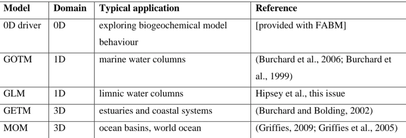
FABM has been coupled to a range of hydrodynamic models. These include models for 1D marine and limnic water columns, and 3D estuaries, coastal systems, ocean basins and the world ocean. Additionally, FABM comes with a 0D driver that represents a well-mixed box, which can be forced with time series of environmental variables to allow fast testing of biogeochemical models. An overview of supported host models is provided in Table 1. Commitments have also been made to couple FABM to the widely used NEMO ocean model (Madec, 2008) (Plymouth Marine Laboratory). Table 1. Hydrodynamic models that have been coupled to FABM.
Model Domain Typical application Reference 0D driver 0D exploring biogeochemical model
behaviour
[provided with FABM]
GOTM 1D marine water columns (Burchard et al., 2006; Burchard et al., 1999)
GLM 1D limnic water columns Hipsey et al., this issue GETM 3D estuaries and coastal systems (Burchard and Bolding, 2002) MOM 3D ocean basins, world ocean (Griffies, 2009; Griffies et al., 2005) Coupled biogeochemical models
FABM includes several biogeochemical models, which vary from compact planktonic ecosystem and suspended matter models to the comprehensive AED and ERSEM ecosystem models. Additionally, proofs of concept are provided that include a single passive tracer models, and a benthic predator that can be coupled to a pelagic model. An overview of supported biogeochemical modules is given in Table 2.
Additionally, FABM is used for development of in-house biogeochemical models across a range of institutes that include the Leibniz Institute for Baltic Sea Research, the Helmholtz-Zentrum
21
Institutt for Vannforskning, the Tallinn University of Technology, the University of Western Australia, , the University of Victoria, and the Plymouth Marine Laboratory.
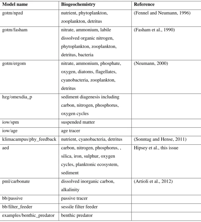
Table 2. Biogeochemical models in FABM. This table lists production-ready models only; it excludes several examples and proof-of-concepts included with FABM.
Model name Biogeochemistry Reference
gotm/npzd nutrient, phytoplankton, zooplankton, detritus
(Fennel and Neumann, 1996)
gotm/fasham nitrate, ammonium, labile dissolved organic nitrogen, phytoplankton, zooplankton, detritus, bacteria
(Fasham et al., 1990)
gotm/ergom nitrate, ammonium, phosphate, oxygen, diatoms, flagellates, cyanobacteria, zooplankton, detritus
(Neumann, 2000)
hzg/omexdia_p sediment diagenesis including carbon, nitrogen, phosphorus, oxygen cycles
iow/spm suspended matter
iow/age age tracer
klimacampus/phy_feedback nutrient, cyanobacteria, detritus (Sonntag and Hense, 2011)
aed carbon, nitrogen, phosphorus, ,
silica, iron, sulphur, oxygen cycles, planktonic ecosystem, sediment
Hipsey et al., this issue
pml/carbonate dissolved inorganic carbon, alkalinity
(Artioli et al., 2012)
bb/passive passive tracer
bb/filter_feeder sessile filter feeder examples/benthic_predator benthic predator Bindings for other programming languages
FABM is written in Fortran 2003 to facilitate simple, high-performance coupling to Fortran-based hydrodynamic models, while retaining the ability to use object-oriented programming concepts. Nevertheless, it is possible to couple to Fortran 2003 code from other programming languages, including C, Python, R and MATLAB. Such “bindings” can be used to either obtain access to
22
FABM’s biogeochemical process descriptions from an alternative language, or to provide FABM with new biogeochemical models coded in an alternative language. In the first case, the binding fulfils the role of a hydrodynamic model; in the second case, the binding fulfils the role of a biogeochemical model (cf. Fig 1).
In general, the process of coupling FABM to another programming language is identical to coupling FABM to a new hydrodynamic or biogeochemical model, with the exception that the binding may require a compatibility layer that converts FABM’s object-oriented constructs to Fortran 90. This is demonstrated with a simple FABM driver, written in Python and supplied with FABM. This driver calls FABM to initialize a biogeochemical model configuration, enumerate all associated parameters and variables, and to retrieve sink and source terms. When combined with Python-based time integration, this functionality can be used to perform a 0D model simulation from Python. A similar approach can be used to couple a biogeochemical model written in an alternative
programming language to FABM, thus gaining the ability to embed this biogeochemical model in a variety of hydrodynamic models. This scenario is particularly feasible if the biogeochemistry is coded in a lower-level programming language (e.g., C or C++), or if computational cost is not an issue. The overhead associated with high-level languages such as Python, R and MATLAB makes them
unsuitable for computationally critical components such as sink-source calculations. For instance, while it is technically possible to combine a Fortran-based global circulation model with
biogeochemistry coded in MATLAB, the associated computational cost is likely to make this scenario non-viable in practice.
Development of the framework
FABM is actively being developed, with new features added at regular intervals. Development occurs in a transparent manner: proposed changes are described in detail in “Requests for Comments”, published on FABM wiki pages and announced on the developers’ mailing list. Implemented updates are documented in individual “API update” notes, which describe any changes that must be made to coupled hydrodynamic and biogeochemical models. The current Application Programming Interfaces (APIs) offered by FABM are regarded as mature, and future updates are expected to preserve
compatibility with existing coupled models. Backward compatibility with biogeochemical models in particular is a leading principle in further development of the framework.
In the short term, updates to the API are planned that will simplify model configuration, both by reducing the number of source lines needed to register biogeochemical variables and parameters during initialization, and by simplifying the format of files that provide FABM’s run-time configuration. Interfaces for run-time information exchange will be expanded to enable complete configuration of FABM through Graphical User Interfaces (GUIs). This will be demonstrated within
23
the GUI for the General Ocean Turbulence Model. Ultimately, this functionality could also be used to enable configuration of biogeochemistry through web interfaces, and to add a GUI to FABM’s 0d driver. In the long run, we envisage using FABM to drive changes in the number and attributes of particles in individual or agent-based models, which are regularly used in aquatic ecosystem studies (Huse et al., 2004; Woods, 2005). To make this possible, FABM interfaces may be extended to include more explicit treatment of particles and their properties.
Additional functionality for biogeochemical models will also be implemented. This includes full support for coding multiple-band irradiance and light absorption models within FABM. Functionality will also be added to enable biogeochemical models to define arbitrary new dimensions (e.g.,
sediment depth, species size, wavelength of irradiance).
The run-time coupling abilities of FABM will also be extended. Currently, FABM only supports one-to-one coupling between biogeochemical variables: it couples models by merging their variables. This will be extended to allow one-to-many coupling (e.g., multiple phytoplankton species serving as prey for a single zooplankton species), and to apply an optional scale factor to coupled variables. The latter can be used to handle differences in units between models, and can also be used to represent different contributions in one-to-many coupling (e.g., different preferences for the phytoplankton species consumed by a single predator).
Discussion: other coupling frameworks
Several other software frameworks have been developed to facilitate model coupling. These couplers include OASIS, the Earth System Modeling Framework (ESMF), the Model Coupling Toolkit (MCT), and other Fortran-based software designed for earth system modelling (Valcke et al. 2012), as well as non-Fortran solutions such as the Open Modeling Interface (OpenMI). Most of these couplers can be used with Fortran code, and have over time been generalized to enable exchange of arbitrary data between software components. Superficially, this functionality seems very similar to that of FABM. In fact, FABM does feature components found in other couplers, such as a central registry of available fields and the logic to couple such fields at run-time. This could lead one to think that FABM might be re-implemented as a set of biogeochemistry-specific APIs around an existing coupler. However, there are good reasons to view FABM and other couplers as complementary technologies, the former more suitable for coupling of processes within a single physical domain, the latter more suitable for generic coupling between domains.
Foremost, most other couplers associate their components with a specific spatial grid, time stepping scheme, domain decomposition, and set of computer cores. This reflects the fact that traditionally, different coupled components described different physical domains (e.g., land, ocean, ice,
24
grids, time stepping and scheduling, and efficient parallel data transfer between cluster nodes. This is very different from FABM, which provides a local description of biogeochemical processes only, independent of a specific spatiotemporal context. FABM is designed to run transparently within a host model that defines the spatial domain and a time loop; the combination of host and FABM could amount to model component in other couplers. This is exemplified by the development of an ESMF biogeochemistry component that links FABM to a generic 3D grid (Richard Hofmeister, Helmholtz-Zentrum Geesthacht, personal communication).
Moreover, data exchange in FABM is very different from that in other couplers. Due to its local process description, different biogeochemical models active within FABM operate on the same spatial grid. Thus, data exchange between models does not require spatial interpolation. Data exchange is further simplified by calling the different biogeochemical components sequentially, thus guaranteeing that all exchanged data reside in the same memory space. Parallelization can be efficiently handled at a higher level, typically by the host through domain composition. As coupled models share the same grid and run on the same compute node, data exchange between biogeochemical models can be completely handled through shared memory. Models are not required to call separate subroutine calls for getting or setting data as used in other couplers; instead, the framework updates data pointers used by biogeochemical modules, thus ensuring that always point to the appropriate fields. There is no need for the advanced interpolation and communication logic provided by other couplers; in the best case, they would simply to fall back to shared memory, in the worst case overhead could increase dramatically. At present, the use of separate frameworks for direct within-domain coupling (FABM for biogeochemistry) and managed between-domain coupling (ESM couplers) are likely the
computationally most efficient solution. FABM’s emphasis on process coupling within a single domain is similar to that of MESSy (), which is used predominantly in atmospheric chemistry. A key difference between FABM and MESSy is that FABM explicitly targets tracers and abstracts all information on the spatial domain, whereas MESSy more generically views its components as operators that can perform any action on its fields. An
Model coupling is a dynamic field that moves rapidly with advances in computer technology. Increases in model performance are increasingly obtained by adding more processor cores, which demands further parallelization of computations. Traditional separation of physical domains combined with domain decomposition may not suffice to meet these demands. Additional parallelization of computations within domains (e.g., by allowing parallel computation of ocean hydrodynamics and biogeochemistry, but also of individual biogeochemical processes) may be needed to better exploit future high performance computing systems. To enable this, couplers are adding logic for efficient, parallel data exchange of large (3D) fields (e.g., MCT, OASIS3-MCT). On the biogeochemistry side, these developments could ultimately lead to a coupler that assigns each biogeochemical process to separate set of compute nodes. This level of modularity agrees well with that pursued by FABM, and
25
it is conceivable to build this new coupler based on FABM APIs using existing software (e.g., MCT) for parallel data exchange. Thus, biogeochemical models that are coded now against FABM APIs seem well prepared for future changes in HPC environments.
Conclusions
A general programming framework for biogeochemical models must balance ease-of-use, flexibility and performance. It is also subject to external constraints, such as the functionality that hydrodynamic models can provide, and the programming language they are written in. Acknowledging these issues, we have designed FABM as a Fortran-based, light-weight coupler that places minimal restrictions on hydrodynamic and biogeochemical models. It achieves its design goals: biogeochemical model codes run unmodified in a variety of hydrodynamic models, performance is comparable to that of custom tailored physical-biogeochemical couplings, comprehensive biogeochemical models can be developed in the form of many compact, self-contained modules, and the final coupled biogeochemistry model can constructed at run-time by non-programmers. FABM makes it possible to partition development tasks and places maximum control in the hands of end-users. These features facilitate large scale collaborations between scientists, programmers and end-users.
Acknowledgements
From 2008 till 2011, development of FABM was funded by the Theme 6 of the EC seventh framework programme through the “Marine Ecosystem Evolution in a Changing Environment” project (MEECE, project no. 212085). Concepts used in FABM were developed during work on a GOTM-biogeochemistry coupler in 2008, funded by the Helmholtz-Zentrum Geesthacht, Centre for Materials and Coastal Research, Germany.
References
Artioli, Y., Blackford, J.C., Butenschon, M., Holt, J.T., Wakelin, S.L., Thomas, H., Borges, A.V., Allen, J.I., 2012. The carbonate system in the North Sea: Sensitivity and model validation. Journal of Marine Systems 102 1-13.
Baretta, J.W., Ebenhöh, W., Ruardij, P., 1995. The European Regional Seas Ecosystem Model, a complex marine ecosystem model. Netherlands Journal of Sea Research 33(3-4) 233-246.
Blackford, J.C., Gilbert, F.J., 2007. pH variability and CO2 induced acidification in the North Sea.
Journal of Marine Systems 64(1-4) 229-241.
Burchard, H., Bolding, K., 2002. GETM: A General Estuarine Transport Model. Scientific Documentation, Tech. Rep., EUR 20253 EN. European Commission.
Burchard, H., Bolding, K., Kuhn, W., Meister, A., Neumann, T., Umlauf, L., 2006. Description of a flexible and extendable physical-biogeochemical model system for the water column. Journal of Marine Systems 61(3-4) 180-211.