Vol. 8, No. 3, pp 77-94 Summer 2015
A Comparison of Regression and Neural Network Based for Multiple
Response Optimization in a Real Case Study of Gasoline Production
Process
M. Bashiri
1*, H. R. Rezaei
1, A. Farshbaf Geranmayeh
1, F. Ghobadi
31. Department of Industrial Engineering, Faculty of engineering, Shahed University, Tehran (Iran) 3. Department of Chemical Engineering, Isfahan University of Technology, Isfahan (Iran)
Abstract
Most of existing researches for multi response optimization are based on regression analysis. However, the artificial neural network can be applied for the problem. In this paper, two approaches are proposed by consideration of both methods. In the first approach, regression model of the controllable factors and S/N (signal to noise) ratio of each response has been achieved, and then a fuzzy programming has been applied to find the optimal factors' levels. In the second approach, a tuned Artificial Neural Network (ANN) is used to relate controllable factors and overall exponential desirability function then genetic algorithm (GA) is used to find factors’ optimum values. Mentioned approaches have been discussed in a real case study of oil refining industry. Experimental results for the suggested levels confirm efficiency of the both proposed methods; however, the Neural Network based approach seems to be more suitable for our case study.
Keywords: Multi-response optimization, Taguchi method, Artificial Neural Network, Genetic Algorithm, Fuzzy programming.
1- Introduction
Many processes around us need to be analyzed for their performance improvement. The analyzer is interested in optimizing processes with minimal experiments and the least cost. Taguchi method (Taguchi, 1991) is an important technique in design of experiment and is used in many case
*Corresponding author.
ISSN: 1735-8272, Copyright c 2015 JISE. All rights reserved
studies we are dealing with them. Taguchi method can be carried out based on a few periods of time and low number of experiments; also, it is a useful and coincident method for industrial experiments. The Taguchi method of robust parameter design is an offline statistical quality control
technique in which the level of controllable factors or input process parameters are so chosen to nullify the deviation in responses due to uncontrollable or noise factors such as humidity, vibration and environmental temperature (Taguchi, 1991; Podder et al., 2001).
Today's studies in Taguchi method usually have focused on multi response optimization. Recently, Taguchi method has been combined with complementary approaches to solve multi-response problems. Some prior approaches in multi-multi-response optimization with Taguchi method have used weighted SN ratio approach (Gauri and Chakraborty, 2010; Gauri and Pal, 2010). Meta-heuristic algorithms have been applied to calculate weight of each response (Jeypaul et al. 2006), moreover, multi criteria decision-making (MCDM) (Lan, 2009), grey rational analysis (GRA) (Lin and Tarng, 1998) and principal component analysis (PCA) (Tong et al. 2005) have been used to optimize responses. In addition, some researchers have focused on multiple response optimizations by ANN (Chang, 2008; Chang and Chen, 2011). Some of mentioned approaches have been more illustrated in the next section.
In this study, we evaluate two approaches based on regression model and neural network respectively. In the first approach, Combination of Taguchi method, Analytical Hierarchy Process (AHP) technique and fuzzy programming have regarded to evaluate the quality of achieved optimal levels. In this approach, regression model is used to find the relation function between controllable factors and S/N ratio of each response. Then, response weights derived by AHP are used as objectives' coefficients in fuzzy programming. In the second approach, the relation between controllable factors and response variables is trained by a neural network and then optimal factors' levels are determined by Genetic Algorithm considering overall desirability. It is worth to mention that the Taguchi method is used for tuning the ANN parameters.
The rest of this paper is organized as follows: section 2 reviews some of existing works on multiple response problems using Taguchi method and ANN. The details of the proposed methods are expounded in section 3. The proposed approaches have been more illustrated as an application in the Gasoline production process in Section 4. Efficiency of the proposed methods by a confirmation experiment and its analysis has been reported in section 5 and finally, the conclusion remarks are discussed in section 6.
2- Literature review
In this section literature review of multi response optimization approaches based on Taguchi method and ANN have been surveyed. Also, the usage of Taguchi method for tuning the parameters of ANN has been considered. In previous works, many studies have been done to optimize single response problems by using Taguchi method (Al-Refaie, 2009; Li et al., 2009). Recently, more studies have tended to multi- response problems. In this regards, weighted SN ratio (WSN) has been used to transform all of SN ratios in each treatment to the unique value for more easily decision (Gauri and Chakraborty, 2010; Gauri and Pal, 2010). Also, meta-heuristic algorithms have been used to attain desirable factors' levels for achieving best responses. Jeypaul et al. (2006) have presented an approach for computing the response weights based on maximization of total weighted S/N ratio which has been considered as GA fitness function. Frequently, gray rational analysis (GRA) in Taguchi method has been reported as an efficient approach to choose the best design factors in multi response problems (Lin and Tarng, 1998). Many researchers have considered this approach for optimizing factors' levels and grey rational optimization is most commonly used in real cases (Manivannan et al., 2011; Al-Refaie, 2010). Since multiple regression models are useful
Multi attribute decision-making approaches are other methods which have been studied in previous researches, in this regard; TOPSIS (technique for order preference by similarity to ideal solution) have been used to determine the best levels (Lan, 2009). In addition to TOPSIS, They used mean effects for S/N ratios for determining best levels to achieve the turning parameters. Kuo et al. (2010) have used Taguchi method to design the experiment and they have employed hierarchical structure of the AHP technique to establish the positive comparison matrix, for more information see (saaty, 1980; saaty et al., 1989). After consistency verification, global weight calculation, and priority sequencing, the optimal multi-attribute parameter has been obtained.
The main problem which occurs is that when the mean square error (MSE) of the regression model is a high value, the ability of the model to describe the relationship of the response variable and the controllable factors would be poor (Kim et al., 2001). For overcoming this problem ANN can be used as a proper substitute method for response estimation. Some authors have compared response surface and regression models with ANN in model building and the preciseness of ANN has been verified in their results (Erzurumlu & Oktem, 2007; Tsao, 2008; Desai et al., 2008; Namvar-Asl et al., 2008). In other hand, to obtain better performance of ANN, tuning some effective parameters seems necessary. However, a proportion of researches in this area have chosen these parameters by try and error, while there are some methods based on design of experiments to tune effective parameters (Sukthomya & Tannock, 2005; Yum & Kim, 2004; Tortum et al., 2007; Bashiri & Farshbaf Geranmayeh, 2011). In this paper, optimum parameters of ANN are obtained using Taguchi method. For this purpose, at first determining performance criterion of ANN and effective parameters in it is essential. Some of the published works have used ANN in multiple response optimizations. Gutierrez and Lozano (2010) have obtained the most efficient treatment by using ANN and CCR Data Envelopment Analysis (DEA) model. Noorossana et al. (2009) first used radial based function (RBF) neural network to determine the set of effective parameters and by multi-layer perceptron neural network they estimated the relation between determined effective parameters and response variables and finally have obtained optimum treatment by applying desirability function and GA. Chang (2008) proposed an approach using data mining, ANN, desirability function and SA for optimizing a dynamic multi response problem. Chang and Chen (2011) used ANN to approximate relation between controllable factors and responses. They computed optimum values by using the overall desirability function and genetic algorithm. Lin et al. (2012) have compared integration of neural network, desirability function and genetic algorithm to find optimal combination of parameters’ levels against other methods. Results of this paper show that integrated procedure outperforms Taguchi method and traditional approaches. Sibalija et al. (2011) have converted the quality losses of the correlated responses into uncorrelated components using the Principal Component Analysis (PCA) and then the Grey Relational Analysis (GRA) was applied to synthesis components into a synthetic performance measure. They have applied artificial neural network for estimating the relation between controllable factors and a synthetic performance measure and a genetic algorithm for finding the optimum laser drilling parameters. Sibalija and Majstorovic (2012), in a similar approach, have applied PCA, GRA, ANN and Simulated Annealing (SA) to find the optimal combination of parameters in a multiple response problem. Rong et al (2015) have extended a novel approach based on neural network and genetic algorithm. They have
improved the quality of weld joint and the effect of the proposed design of experiment has been checked in an actual laser brazing process. Their procedure has been done by Taguchi L-25. Then their input factors have been optimized using the couple of back propagation neural network and Genetic algorithm in an interactive method. Koyee et al. (2014) have proposed a novel five-step approach including pre-process of data (design the experimentations base on Taguchi), different MADM techniques (AHP-TOPSIS), converting the crisp inputs to fuzzy trapezoidal numbers, fuzzy additive weighted method and determination of ranks and post-process the numbers. Beigmoradi et al. (2014) have applied Taguchi method to reduce number of simulations to reach optimum values of parameters in a real case study of optimization of rear end of a simplified car model. In their proposed approach, results of Taguchi have been used to obtain a relation between parameters and objectives employing ANNs. The results of the model have been conducted by the ANN and multi objective Genetic Algorithm methods. Finally, flow around the optimized model has been studied by numerical simulation and results have been reported.
As mentioned above, multi response optimization is a useful tool in wide range of problems. Recent studies on Gasoline production have been had less attention to design of experiments. Rezai et al. (2008) have surveyed four controllable factors which affect on flotation of coal. Authors have considered Gasoline as one of the controllable factors. They have reported Taguchi method as more efficient method compared to factorial design. Attending the literature review shows that investigation of multi response optimization in adding materials to base Gasoline is a novel issue. The summery of papers which is surveyed in the literature has been shown in Table 1.
Table 1. The summary of related published works in the literature Taguchi
Method
Artificial Neural Network
Regressio n Model
Complementary solving approach
Gauri and Chakraborty (2010)
Gauri and Pal (2010) * WSN
Jeypaul et al. (2006) * GA
Manivannan et al. (2011)
Al-Refaie, (2010) * GRA
Lan, (2009)
Kuo et al. (2010) * MADM
Al- Refaie et al. (2009b) * * GRA
Gutierrez and Lozano (2010) * * DEA
Noorossana et al. (2009) * Desirability Function & GA
Chang and Chen (2011) * * Desirability Function & GA
Chang (2008) * * Desirability Function & SA
Lin et al. (2012) * * Desirability Function & GA
Sibalija et al. (2011) * * PCA, GRA & GA
Sibalija and Majstorovic (2012) * * PCA, GRA & SA
Rong et al (2015) * * GA& back propagation
neural network
Koyee et al. (2014) * Fuzzy MADM
Beigmoradi et al. (2014) * * -
Proposed approaches * * * Fuzzy Programming, Desirability Function & GA
3- Proposed methods
In this section, two approaches are discussed. The first one is based on regression modeling and Fuzzy Programming and the second one is based on ANN and GA.
3-1- Regression analysis and fuzzy programming
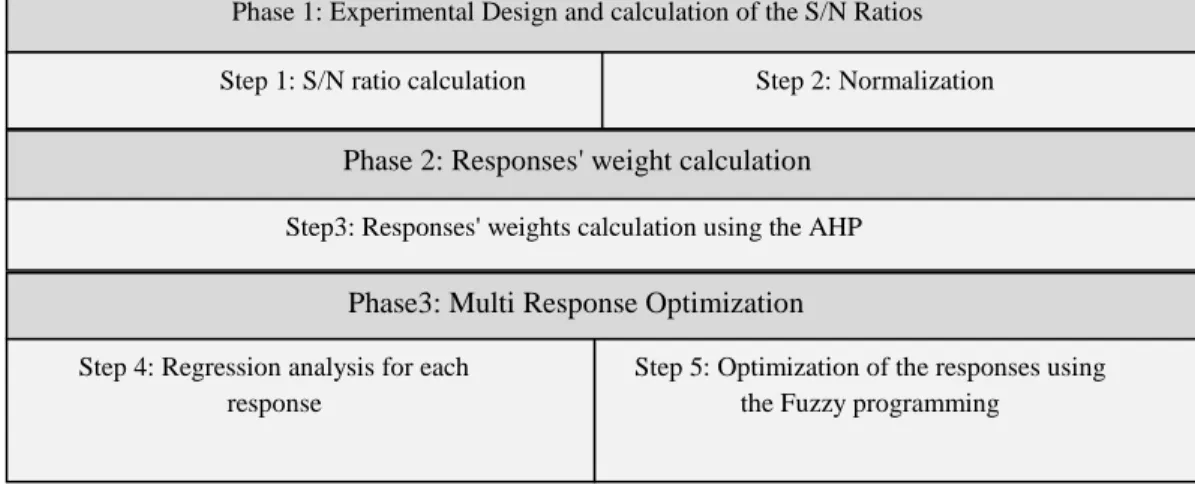
In this section, the proposed method for optimizing S/N ratio of response based on Taguchi method is presented. This approach contains 3 phases as illustrated in Figure 1.
Figure 1. Multi response optimization proposed approach based on Fuzzy Programming
3-1-1- Experimental design and calculation of the S/N Ratios Step1: S/N ratio calculation
For each experiment, calculate S/N ratio value, Lij, at experiment i for response j using an
appropriate equation according to kind of responses (e.g. for larger the better (LTB) use
∑
= −
= n
i yij
n 1
10 ij
1 1 log 10
L ).
Step 2: Normalization
Adopt S/N ratio according to normalizing approach (e.g. for LTB response use appropriate relation)
(
)
(
L ,i 1,2,...,n)
min(
L ,i 1,2,...,n)
maxn ,..., 2 , 1 i , L min L z
ij ij
ij ij
ij = − =
= −
= ).
3-1-2- Responses' weight calculation
In this phase, weight of each response is determined.
Step 3: Responses' weights calculation using the AHP
Compute weight of each response by using AHP technique (saaty, 1980; saaty et al., 1989) and notice that inconsistency ratio would be suitable (less than 0.1).
Phase 1: Experimental Design and calculation of the S/N Ratios Step 1: S/N ratio calculation Step 2: Normalization
Phase 2: Responses' weight calculation
Step3: Responses' weights calculation using the AHP
Phase3: Multi Response Optimization
Step 4: Regression analysis for each response
Step 5: Optimization of the responses using the Fuzzy programming
(1)
3-1-3-Multi response optimization
In this phase, we want to predict each objective function for each response as a regression analysis and optimize the problem based on fuzzy programming as a multi objective decision-making technique.
Step4: Regression analysis for each response
Perform a regression analysis to find the relation function between each response and its factors. Notice that R-sq and Adjusted R-sq should be appropriate for the regression model.
Step5: Optimization of the responses using the Fuzzy programming
Fuzzy programming (for more realization see (Zimmerman, 1978; Cheng et al. 2002)) is considers as following steps:
1- Solve each objective function separately and find the other objectives’ values by the optimal controllable factors.
2- Construct the payoff matrix.
* i
Z is the optimum value of ith objective function andZij is attained by putting the optimal value of
variables of Ziin the jth objective function.
3- Defineµ
( )
Zj as linear membership function for jth objective function according to (3).Where, ∆j=Uj−Ljis acceptable tolerance for each objective function (Zj).
4- Solve the fuzzy programming model as (4)-(6).
(4) ∑wi i
Max α
(5) k
i=1,2,...,
i i
i i
L U
L Z
− − ≤ α
(6) k
i=1,2,...,
(
n)
ii x x x b g 1, 2,..., ≤≥
Where wi is the weight of each jth objective determined by AHP. The best factors’ levels are
obtained from equations (3)-(6).
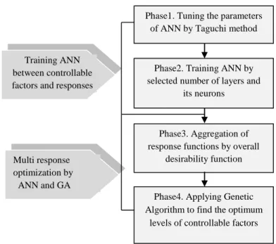
3-2- Artificial neural network
This section contains the proposed approach, which has been illustrated in Figure 2. In the first step, we determine the best number of layers and its neurons, then, by training the neural network, we compute exponential desirability function and finally, Genetic Algorithm is used to find the optimal levels of controllable factors in optimizing the overall desirability function.
( )
zj = µ0 if Zj≤Uj−∆j j
j U Zj j
∆ ∆ −
−( )
if Uj−∆j≤Zj≤Uj 1 if Zj≥Uj
Figure 2. The proposed approach of Multi response optimization by ANN and GA
3-2-1-Tuning the parameters of ANN
During the training a neural network, some parameters must be defined like the number of hidden layers and the number of neurons in each layer; For this purpose, most of recent researches have selected these parameters randomly or by means of trial and error. Tuned neural network has low error for training the relation between controllable factors and response variables, so we select the best parameters of ANN by Taguchi method. For this purpose, numbers of hidden layer in neural network and number of neurons are considered as effective parameters in performance of ANN and Root Mean Square Error (RMSE) between outputs and targets of the neural network is considered as performance criteria. Note that RMSE is a smaller the better (STB) type performance criterion. Ideal value for RMSE is zero where in ANN structure, trained output values are fitted on target values.
Figure 3 shows the structure of ANN and Table 2 shows the ANN’s performance criterion and related effective parameters, which are applied for tuning the parameters of ANN. By analyzing Taguchi, design key levels for each effective parameters in performance of ANN can be computed.
Phase1. Tuning the parameters of ANN by Taguchi method
Phase2. Training ANN by selected number of layers and
its neurons
Phase3. Aggregation of
response functions by overall desirability function
Phase4. Applying Genetic Algorithm to find the optimum
levels of controllable factors Training ANN
between controllable factors andresponses
Multi response optimization by ANN and GA
Input
L a y e r 1
L a y e r 2
Target
Out put
Figure 3. Topology of Black Box in ANN
Table 2. ANN’s performance criterion and related effective parameters
Effective parameters Performance criterion
The number of neurons in the first and second hidden layer of ANN
RMSE between the outputs and targets of ANN
3-2-2- Training ANN
By obtaining layers status, for predicting the response variables, we need to train the relation between response and its controllable factors. Therefore, one of the existing treatments is selected as test treatment and others are selected for ANN training. If we have more than one response variable, for simplifying, we could train one neural network for each response.
3-2-3- Aggregation of responses by overall desirability function
To optimize several responses simultaneously, desirability function technique is represented (Del Castillo et al. 1996). The desirability function transforms value of response to scale free-value and denotes it as di for ith response. Desirability function’s value is between 0 and 1. The more di close to one, the more desirable response is (Jeong and Kim, 2009). Derringer and Suich (1980) defined this function for a nominal-the best (NTB) type response.
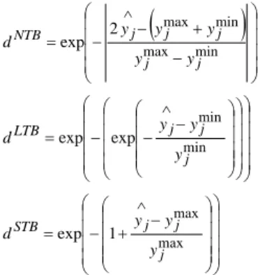
In this paper, we use exponential desirability function for determining the desirability value of each response variable, separately. The formulas for each type of response (i.e. LTB, STB and NTB) are given in equations (7), (8) and (9).
(
)
− + − − = ∧ min max min max 2 exp j j j j j NTB y y y y y d (7) − − − = ∧ min min exp exp j j j LTB y y y d (8) − + − = ∧ max max 1 exp j j j STB y y y d (9)Whereyminj and max j
y are the lower and upper bounds of the selected response, respectively. y∧j is
approximated value of response which is obtained as output of ANN. But for a final decision, we need to have a total objective function based on each desirebility function. For this porpose, Harrington (1965) proposed a geometric mean in order to aggregate individual desirability functions and approach to overall desirability function D. Then the optimal combination set of factors is determined by maximizing D. In this study, weighted geometric mean, which is proposed by Derringer (1994), is used according to Equation (10).
(
)
∑= dWd W dIWI Wi
D
1 2
1 1 2... (10)
3-2-4- Applying Genetic Algorithm to find optimum combination of controllable factors
Genetic algorithm has been proved to be a successful method for solving LP and NLP problems inspired by the process of natural selection and genetic evaluation. GA applies mutation, crossover and selecting operators to a population of encoded parameters space. The algorithm searches different areas of the parameters space and guides the solution to the region where there is a high probability of global optimum. For studying more about genetic algorithm see (Ahn, 2006). In proposed method, after establishing overall desirability function according to the desirability of each response, GA is applied for finding the optimum combination set of controllable factors.
4- A real case study in gasoline production process
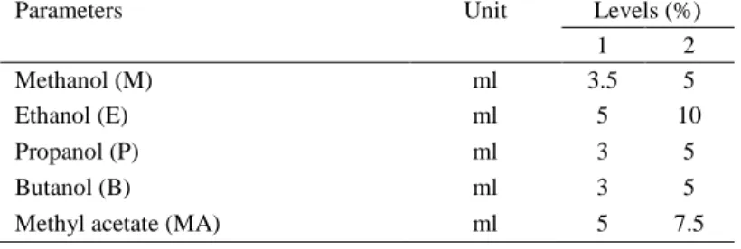
Mentioned approaches have been implemented in a real case study of Isfahan oil refining company and the results have been reported and analyzed in this section. The factors and their levels considered in this study are shown in Table 3. Experiments are conducted with five controllable factors each at two levels. Also we tested 8 treatments with 2 replicates given in Table 4. Rate of octane number (RON), rapid vapor pressure (RVP) and density are considered in this research as interested responses, which are LTB, STB and LTB, respectively.
Table 3. Controllable factors and their levels for the case study
Parameters Unit Levels (%)
1 2
Methanol (M) ml 3.5 5
Ethanol (E) ml 5 10
Propanol (P) ml 3 5
Butanol (B) ml 3 5
Methyl acetate (MA) ml 5 7.5
Table 4.L8 Orthogonal array for designed experiment and response values for the case study
Trial No. M E P B MA Responses (2 replicates)
RVP RON DENSITY
1 1 1 1 1 1 64 63 89 88.3 0.7507 0.7510
2 2 2 1 1 1 63 62.5 93.5 92.4 0.7550 0.7553
3 1 1 2 2 1 62 60.5 88 87.1 0.7530 0.7535
4 2 2 2 2 1 61.5 60.5 94 93 0.7557 0.7561
5 2 1 2 1 2 63 62 93.2 92.1 0.7585 0.7590
6 1 2 2 1 2 62.5 61.5 91.8 91 0.7560 0.7563
7 2 1 1 2 2 62 61 93.5 92.4 0.7583 0.7587
8 1 2 1 2 2 61 59.5 91.5 90.5 0.7566 0.7568
In the both approaches in the section 4.1 and 4.2, response weights derived from AHP are used. So Table 5 shows the allocated values in comparison matrix (CM) by standpoint of chemical engineering specialist. Also in Table 6, weights of each response and inconsistency ratio (IR) have been reported.
Table 5. Comparison matrix for response weights calculation in Analytical Hierarchy Process
RON RVP DENSITY
RVP
6
1 1 2
DENSITY
9 1
2 1
1
Table 6. Calculated weights for each response of the case study
Response Weight value
RON 0.779
RVP 0.143
DENSITY 0.079
Inconsistency Ratio(IR)=0.01
In the next sections (4.1 and 4.2) multiple response optimization approaches on case study are illustrated.
4-1- Multi response Optimization Based on Regression analysis and Fuzzy
Programming.
In this approach, the experiments are studied using L8 orthogonal array which is presented in
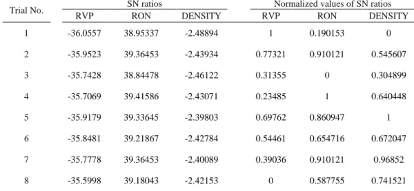
Table 4. According to kind of each response, proportionate equation are used to compute SN ratios and their normalized values (e.g. for RON, LTB formula is appropriate in S/N computation). Table 7 shows the SN and normalized SN ratios for each response of each treatment.
Table 7. S/N and Normalized S/N ratio values for the Gasoline production process case study
Trial No. SN ratios Normalized values of SN ratios
RVP RON DENSITY RVP RON DENSITY
1 -36.0557 38.95337 -2.48894 1 0.190153 0
2 -35.9523 39.36453 -2.43934 0.77321 0.910121 0.545607
3 -35.7428 38.84478 -2.46122 0.31355 0 0.304899
4 -35.7069 39.41586 -2.43071 0.23485 1 0.640448
5 -35.9179 39.33645 -2.39803 0.69762 0.860947 1
6 -35.8481 39.21867 -2.42784 0.54461 0.654716 0.672047
7 -35.7778 39.36453 -2.40089 0.39036 0.910121 0.96852
8 -35.5998 39.18043 -2.42153 0 0.587755 0.741521
At this stage, the regression analysis result has been reported in Table 8. R-square and adjusted R-square confirm that the additive model is fitted to the experimental data.
Table 8. Regression model between the S/N ratio of each response and controllable factors
Response Regression relation R-square value (%)
RON 1.97+0.375M+0.0596E+0.0913MA R-Sq=97.3, R-Sq(adj)=95.2
RVP 2.28-0.0424E-0.26B-0.0689MA R-Sq=94,R-Sq(adj)=89.5
Density -1.59+0.239M+0.189MA R-Sq=91.3,R-Sq(adj)=87.8
In the above regression analysis, 90% of confidence level has been set, so deleted factors have no significant effect in this analysis.
Pay off matrix of the case study
Table 9.
RON RVP Density
(
M *,E *,P*,B *,MA*)
RON 1.1* 0.56 1 (5,10,3,3,7.5)
RVP 0.097 0.94* 0.19 (3.5,5,3,3,5)
Density 0.88 0.77 1* (5,5.3,3,7.5)
Lower bound 0.097 0.56 0.19
Upper bound 1.1 0.94 1
According to equations (1) – (4), the problem is solved by classic optimization software and results are given in table 10.
Table 10. Optimum factors levels which are obtained by the proposed approach
Factor M E P B MA
Selected coded
Level 2 2 1 1 2
Uncoded Value 5 10 5 3 7.5
As it is obvious in Table 10, M2 E2 P1 B1 MA2 is optimum solution for case study.
4-2- Multi response optimization based on ANN
In this approach, the first phase is tuning the parameters of ANN. For this purpose, a Taguchi
design based on two controllable factors and one response variable is considered. The first factor is the number of neurons in layer 1 and the second is the number of neurons in layer 2. Notice that if the quality of network with the second layer would be better, we will choose it and its neurons, so, if the number of neurons in layer 2 would be equal to zero, layer 1 is sufficient for ANN structure. Root of mean square errors (RMSE) is most important index for evaluation of the quality of ANN parameters (i.e. the number of layers and its neurons). Hence, RMSE is introduced as the response and we want to find the best level of parameters (controllable factors) with consideration of minimum RMSE (smaller the better response). Table 11 shows the levels at each controllable factor and desirable response variables. Also, Table 12 illustrates treatments contains Taguchi design of experiment, level of controllable factors and RMSE result in each treatment. Since we have three responses in this case study, so we should tune three ANN structure parameters.
Table 11. summary of controllable factors and response variable
Performance index for ANN (Response variable) Levels of Controllable Factors
RMSE Controllable factor 2
(Neurons No. in layer 2) Controllable factor 1
(Neurons No. in layer 1)
6 3 0 13
8 3
Table 12. Orthogonal Arrays for tuning the parameters of ANN
Trt Neurons in layer 1 Neurons in layer 2 RMSE(RVP) RMSE(RON) RMSE(DENSITY)
1 3 0 0.72566 1.02783 0.0014139
2 3 3 0.99049 1.07238 0.0019992
3 3 6 0.94183 1.53496 0.0011413
4 8 0 1.45209 2.25732 0.0023611
5 8 3 0.71466 2.65749 0.0014734
6 8 6 1.13604 2.16779 0.0021009
7 13 0 1.74704 2.58517 0.0038092
8 13 3 1.54758 1.23292 0.0024986
9 13 6 1.65974 4.96190 0.0061913
The result of Taguchi analysis selects two hidden layers for ANN structure with three neurons at each layer. Details of this analysis are given in Table 13. As it is clear in Table 13, the first level is more suitable (maximum mean value) for neuron number in layer one in all networks. Also, the second level is suggested as the best number of neurons in second layer for all three networks.
Table 13. Details of analysis for selection of best number of neurons according to Taguchi method
Effective parameters in performance of ANN
Mean value of Taguchi method for number of
neurons in layer1
Mean value of Taguchi method for number of
neurons in layer2
ANN parameters for RVP
1 1.1296* -1.7669
2 -0.4766 -0.2640*
3 -4.3466 -1.6627
ANN parameters for RON
1 -1.522* -5.187
2 -7.427 -3.638*
3 -7.994 -8.118
ANN structure for Density
1 56.61* 52.64
2 54.24 54.22*
3 48.2 52.19
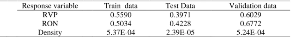
By considering obtained number of layers and their neuron number, neural network is trained. For this purpose, the first replicate of the experiments (reported in Table 4) is supposed as the test data and its second replicate is considered as validation data. RMSE results for the neural networks are presented in Table 14.
Table 14. RMSE results for the training, test and validation data for each network
Response variable Train data Test Data Validation data
RVP 0.5590 0.3971 0.6029
RON 0.5034 0.4228 0.6772
Density 5.37E-04 2.39E-05 5.24E-04
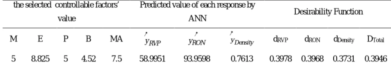
After training the neural network, for applying desirability function, maximum value of RVP (64) and minimum value of RON (87.1) and Density (0.7507) should be considered in equations (6),(7). Moreover, by using GA for exploring new solutions, 57th generated treatment is better than
Table 15. Results of multiple response optimization by ANN approach
Desirability Function Predicted value of each response by
ANN the selected controllable factors’
value Total D Density d RON d RVP d Density y ∧ ∧ RON y RVP y ∧ MA B P E M 0.3946 0.3731 0.3968 0.3978 0.7613 93.9598 58.9951 7.5 4.52 5 8.825 5
5- Confirmation experiment
After completing the identification of the optimal levels, the confirmation experiment is to be conducted to check the efficiency of the proposed approaches. The real test of achieved values for controllable factors confirmed the optimality of levels, which have been attained. The full information about results of final experiment about two approaches is shown in Table 16. Also, improvement value for treatment which has been calculated based on the proposed approaches has been compared to other treatments which have been tested beforehand (see Table 4). Note that for computing the values of each treatment and comparison between existing treatments and proposed solution, the mean of two replications of existing treatments has been considered.
Table 16. Confirmation Experiment For Checking the Efficiency of Proposed Approaches
Response values by real experiments Improvement of the proposed treatment compared with the other experimental data (%)
Treatments RVP
(STB)
RON (LTB)
DENSITY (LTB)
Regression analysis and Fuzzy Programming
Artificial Neural Network Proposed Treatment based
on ANN 60.08 94.07 0.7608 - -
Proposed Treatment based
on Fuzzy Programming 62.5 94.3 0.7571
-
-
1 63.5 88.65 0.75085 5.255817 5.22716
2 62.75 92.95 0.75515 1.208787 1.264627
3 61.25 87.55 0.75325 5.754538 5.696628
4 61 93.5 0.7559 0.327426 1.0989
5 62.5 92.65 0.75875 1.370138 1.654189
6 62 91.4 0.75615 2.366266 2.597312
7 61.5 92.95 0.7585 0.884313 0.991825
8 60.25 91 0.7567 2.295096 0.840204
Table 16 shows that the proposed treatment obtained by mentioned approaches are better than the others (the reported values are sum of the improvements in the responses at each treatment). For example, this table specifies that according to the experimentation results, improvement of selected treatment in Fuzzy programming approach is 5.75% and 0.33 % better than others in the best and worst case respectively.
Moreover, for comparison of two mentioned approaches based on weight of response variables, comparison of regression analysis and ANN approach is shown in Table 17. According to the results, ANN works better than Fuzzy Programming approach in our Gasoline production case.
Table 17. Comparison of two approaches in the Gasoline production case
Overall Desirability Function Total weighted Normalized response values
Fuzzy Programming 0.77575 0.849488
ANN 0.779031 0.947441
6- Conclusion and remarks
In this paper, two approaches for multi response optimization were proposed. In the first approach which is based on regression analysis, after computing S/N ratio for each response, its regression model between normalized S/N ratio and controllable factors were achieved. The entire regression models ware considered as fuzzy programming objective function and then, by using AHP weights of response variables, factors’ levels were optimized. In the second approach, after tuning the ANN parameters, existing experiments were applied for training the neural network, then, by defining desirability function, controllable factors’ optimal value were determined by GA. We implemented two approaches in a case study on adding the additive material to base Gasoline and confirmation experiments showed that both of approaches are efficient. Comparison of two approaches shows that ANN approach is better than regression analysis and fuzzy programming in this case study. Proposed treatment in both approaches saves the economic resulting from decreasing amount of additive material in base Gasoline and increasing the quality of responses especially octane number of Gasoline rather than other treatments.
Acknowledgment
The authors would like to thank Esmaeel Nazem and Mohsen Moradmand for providing the authors with valuable assistance in the case study reported in this paper. Also, the authors want to express deepest gratitude to Dr Mohammad Reza Ehsani and Dr Abdolhossein Dabbagh for cooperating us in chemical engineering concepts of this research.
References
Ahn C. (2006), Advances in evolutionary algorithms: theory design and practice; Springer Verlag. Al-Refaie A. (2009), Optimizing SMT performance using comparisons of Efficiency between different systems technique in DEA; IEEE Transactions on Electronics Packaging Manufacturing
32, 256-264.
Al-Refaie A., Al-Durgham L. & Bata N. (2009), Optimal Parameter Design by Regression Technique and Grey Relational Analysis; Proceedings of World Congress on Engineering, London, U.K.
Manufacture 224, 147-158.
Bashiri M. & Farshbaf Geranmayeh A. (2011), Tuning the parameters of an artificial neural network using Central composite design and genetic algorithm; Scientia Iranica 18, 1600-1608.
Beigmoradi S., Hajabdollahi H. & Ramezani A.(2014), Multi-objective aero acoustic optimization of rear end in a simplified car model by using hybrid Robust Parameter Design, Artificial Neural Networks and Genetic Algorithm methods, Journal of Computers & Fluids 90,123-132.
Chang H. (2008), A data mining approach to dynamic multiple responses in Taguchi experimental design; Expert Systems with Applications 35, 1095-1103.
Chang H. & Chen Y. (2011), Neuro-genetic approach to optimize parameter design of dynamic multiresponse experiments; Applied Soft Computing 11, 436-442.
Cheng Chi. Bin., Cheng C. J. & Lee E. S. (2002), Neuro-Fuzzy and Genetic Algorithm in Multiple response optimization; Computers and Mathematics with Applications 44, 1503-1514.
Del Castillo E., Montgomery D. C. & McCarville D. (1996), Modified desirability functions for multiple response optimization; Journal of Quality Technology 28, 337-345.
Derringer G. & Suich R. (1980), Simultaneous optimization of several response variables; Journal of Quality Technology 12, 214-219.
Derringer G. (1994), A balancing act: optimizing a product's properties; Quality Progress 27, 51-60.
Desai K., Saudagar, S.P., Lele, S. & Singhal, R. (2008), Comparison of artificial neural network (ANN) and response surface methodology (RSM) in fermentation media optimization: Case study of fermentative production of scleroglucan; Biochemical Engineering Journal 41, 266-273.
Erzurumlu T. & Oktem, H. (2007), Comparison of response surface model with neural network in determining the surface quality of moulded parts; Materials and design 28, 459-465.
Gauri S. K., & Chakraborty, S. (2010), A study on the performance of some multi-response optimization methods for WEDM processes; The International Journal of Advanced Manufacturing Technology 49, 155-166.
Gauri S. K., & Pal S. (2010), Comparison of performances of five prospective approaches for the multi-response optimization; The International Journal of Advanced Manufacturing Technology 48, 1205-1220.
Gutierrez E. & Lozano S. (2010), Data Envelopment Analysis of multiple response experiments;
Applied Mathematical Modelling 34, 1139-1148.
Harrington Jr. E. (1965), The Desirability Function; Industrial Quality Control 21, 494-498.
Jeong I. & Kim K. (2009), An interactive desirability function method to multiresponse optimization; European Journal of Operational Research 195, 412-426.
Jeypaul R., Shahabudin P. & Krishnaiah K. (2006), Simultaneous optimization of multi response problems in the Taguchi method using genetic algorithm; The International Journal of Advanced Manufacturing Technology 30, 870-878.
Kim K.J., Byun J.H., Min D. I.J. Jeong. (2001), Multiresponse surface optimization: concept, methods, and future directions, Tutorial; Korea Society for Quality Management.
Koyee R. D., Eisseler R. & Schmauder S. (2014), Application of Taguchi coupled Fuzzy Multi Attribute Decision Making (FMADM) for optimizing surface quality in turning austenitic and duplex stainless steels; Journal of Measurement 58, 375-386.
Kuo C. F. J., Tu K. H. M., Liang S. W. & Tsai W. L. (2010), Optimization of microcrystalline silicon thin film solar cell isolation processing parameters using ultraviolet laser; Optics & Laser Technology 42, 945-955.
Lan T. S. (2009), Taguchi optimization of multi-objective CNC Machining using TOPSIS;
Information Technology Journal 8, 917-922.
Lin, H. C., Su, C. T., Wang, C. C., Chang, B. H., & Juang, R. C. (2012), Parameter optimization of continuous sputtering process based on Taguchi methods, neural networks, desirability function, and genetic algorithms; Expert Systems with Applications 39(17), 12918-12925.
Lin J. L. & Tarng Y. S. (1998), Optimization of the multi-response process by the Taguchi method with grey relational analysis; The Journal of Grey System 10, 355-370.
Li M. H. C., Al-Refaie A. & Yang C. Y. (2009), DMAIC Approach to Improve the Capability of SMT solder Printing Process; IEEE Transactions on Electronics Packaging Manufacturing 31, 126-133.
Manivannan S., Devi S. P., Arumugam R. & Sudharsan N. M. (2011), Multi-objective optimization of flat plate heat sink using Taguchi-based Grey relational analysis; International Journal of Advanced Manufacturing Technology 52, 739-749.
networks and response surface method; Energy Conversion and Management 49, 2471-2477. Noorossana R., Davanloo Tajbakhsh S. & Saghaei, A. (2009), An artificial neural network approach to multiple-response optimization; The International Journal of Advanced Manufacturing Technology 40, 1227-1238.
Podder T. K., Antonelli G. & Sarkar N. (2001), An Experimental Investigation into the Fault-Tolerant Control of an Autonomous Underwater Vehicle, Journal of Advanced Robotics 15, 505-520.
Rezai B., Sheibi H., Refahi A. & Fatemi Ghomi, M. (2008), Comparison of factorial and Taguchi's methods in optimization of effective parameters of coal flotation; Asian Journal of Chemistry 20, 329-336.
Rong Y., Zhang Z., Zhang G., Yue C., Gu Y., Huang Y., Wang C. & Shao X. (2015), Parameters optimization of laser brazing in crimping butt using Taguchi and BPNN-GA; Journal of Optics and Lasers in Engineering 67, 94-104.
Saaty T. L. (1980), The Analytic Hierarchy Process; McGraw Hill International.
Saaty T. L. Alexander & Joyce. (1989), Conflict Resolution: The Analytic Hierarchy Process; New York: Praeger.
Sibalija, T. V., & Majstorovic, V. D. (2012), An integrated simulated annealing-based method for robust multiresponse process optimization; The International Journal of Advanced Manufacturing Technology 59(9), 1227-1244.
Sibalija, T. V., Petronic, S. Z., Majstorovic, V. D., Prokic-Cvetkovic, R., & Milosavljevic, A. (2011), Multi-response design of Nd: YAG laser drilling of Ni-based superalloy sheets using Taguchi’s quality loss function, multivariate statistical methods and artificial intelligence; The International Journal of Advanced Manufacturing Technology 54(5), 537-552.
Sukthomya W. & Tannock J. (2005), The optimisation of neural network parameters using Taguchi’s design of experiments approach: an application in manufacturing process modelling;
Neural Computing & Applications 14, 337-344.
Taguchi G., (1991), Taguchi Methods, Research and Development; American Suppliers Institute Press, Vol (1).
Tong L. I., Wang C-H. & Chen H. C. (2005), Optimization of multiple responses using principal component analysis and technique for order preference by similarity to ideal solution; The International Journal of Advanced Manufacturing Technology 27, 407-414.
Tortum A., Yayla N., Çelik C. & Gökdaĝ M. (2007), The investigation of model selection criteria in artificial neural networks by the Taguchi method; Physica A: Statistical Mechanics and its Applications 386, 446-468.
Tsao C. (2008), Comparison between response surface methodology and radial basis function network for core-center drill in drilling composite materials; The International Journal of Advanced Manufacturing Technology 37, 1061-1068.
Yum B. & Kim Y. (2004), Robust design of multilayer feedforward neural networks: an experimental approach; Engineering Applications of Artificial Intelligence 17, 249-263.
Zimmerman H. J. (1978), Fuzzy programming and linear programming with several objective functions; Fuzzy sets and systems 1, 45-55.