TO QUEUE OR NOT TO QUEUE:
EQUILIBRIUM BEHAVIOR IN
QUEUEING SYSTEMS
REFAEL HASSIN
Department of Statistics and Operations Research Tel Aviv University
Tel Aviv 69978, Israel [email protected] MOSHE HAVIV Department of Statistics The Hebrew University Jerusalem 91905, Israel, and
Econometrics and Business Statistics The University of Sydney
Sydney NSW 2006, Australia [email protected].
Kluwer Academic Publishers
To the memory of my parents, Sara and
Avraham Haviv To my mother and late father, Fela and
Contents
Preface xi
1. INTRODUCTION 1
1.1 Basic concepts 2
1.1.1 Strategies, payoffs, and equilibrium 2
1.1.2 Steady-state 4
1.1.3 Subgame perfect equilibrium 5
1.1.4 Evolutionarily stable strategies 5
1.1.5 The Braess paradox 5
1.1.6 Avoid the crowd or follow it? 6
1.2 Threshold strategies 7
1.3 Costs and objectives 9
1.4 Queueing theory preliminaries 11
1.5 A shuttle example 14
1.5.1 The unobservable model 14
1.5.2 The observable model 17
1.5.3 Social optimality 18
1.6 Non-stochastic models 19
2. OBSERVABLE QUEUES 21
2.1 Naor’s model 21
2.2 The LCFS-PR model 24
2.3 Social optimization 27
2.4 Profit maximization 29
2.5 Heterogeneous customers 34
2.6 Non-FCFS queues without reneging 36
2.6.1 LCFS 37
2.6.2 EPS and random queues 38
2.7 Discounting 39
2.8 State dependent pricing 40
viii TO QUEUE OR NOT TO QUEUE
2.9 Waiting for the right server 41
2.10 Non-exponential service requirements 42
2.11 Related literature 43
3. UNOBSERVABLE QUEUES 45
3.1 Identical customers 45
3.1.1 Equilibrium 46
3.1.2 Social optimization 47
3.1.3 Profit maximization 49
3.2 Observable vs. unobservable queues 51
3.3 Heterogeneous service values 53
3.4 Heterogeneous service values and time costs 56
3.4.1 Equilibrium 56
3.4.2 Social optimization 57
3.4.3 Class decision 57
3.5 Customers know their demand 58
3.5.1 FCFS 58
3.5.2 EPS 59
3.5.3 Shortest service first 60
3.6 Finite buffer 60
3.7 Multi-server models 62
3.7.1 Homogeneous service values 62
3.7.2 Heterogeneous service values 64
3.7.3 Class decision 67
3.8 Queueing networks 68
3.8.1 The Braess paradox 68
3.8.2 Heterogeneous service values 69
3.8.3 Serial networks with overtaking 70
3.9 Related literature 70
4. PRIORITIES 73
4.1 Observable queues 73
4.1.1 Equilibrium payments 73
4.1.2 Two priority classes 75
4.1.3 Profit maximization 82
4.2 Unobservable queues 83
4.3 Discriminatory processor sharing 86
4.3.1 Two relative priority parameters 86
4.3.2 A continuum of relative priority parameters 87
4.4 Incentive compatible prices 91
4.4.1 Heterogeneous time values 91
4.4.2 Pricing based on externalities 92
Contents ix
4.5 Bribes and auctions 96
4.5.1 Homogeneous customers 97
4.5.2 Heterogeneous customers 100
4.6 Class decision 105
4.7 Related literature 108
5. RENEGING AND JOCKEYING 111
5.1 Reneging in observable queues 111
5.2 Reneging in unobservable queues 115
5.2.1 A single step reward function 115
5.2.2 Convex waiting costs 116
5.2.3 Heterogeneous customers 117
5.3 Jockeying 119
5.3.1 Jockeying and the value of information 120
5.3.2 Expected waiting time 121
5.3.3 Steady-state probabilities 122
5.3.4 The value of information 123
5.4 Related literature 124
6. SCHEDULES AND RETRIALS 125
6.1 Waiting time auctions 125
6.2 ?/M/1 126
6.3 Arrivals to scheduled batch service 129
6.4 Retrials 132
6.4.1 Steady-state probabilities 133
6.4.2 Social optimality 135
6.4.3 Equilibrium 135
6.5 Related literature 139
7. COMPETITION AMONG SERVERS 141
7.1 Unobservable queues with heterogeneous time values 142 7.1.1 Continuous distribution of time values 142
7.1.2 Two time values 143
7.2 Unobservable queues with heterogeneous values of service 144
7.2.1 Single class of customers 145
7.2.2 Multiple classes of customers 146
7.3 Observable queues 147
7.4 Price and priority competition 150
7.5 Search among competing servers 152
7.6 Information based competition 153
7.6.1 Existence of an equilibrium 154
7.6.2 Solution of the model 156
x TO QUEUE OR NOT TO QUEUE
8. SERVICE RATE DECISIONS 159
8.1 Heterogeneous service values 160
8.2 Service rate at a fixed price 162
8.3 Bribes and auctions 163
8.4 Asymmetric information 165
8.4.1 Heterogeneous service values 165
8.4.2 Heterogeneous time values 167
8.5 Observable vs. unobservable queues 168
8.6 Co-production 169
8.6.1 Single class FCFS model 169
8.6.2 Multi-class extensions 171
8.7 Competition among servers 173
8.8 Capacity expansion 174
8.9 Related literature 175
Index
Preface
The literature on equilibrium behavior of customers and servers in queuing systems is rich. However, there is no comprehensive survey of this field. Moreover, what has been published lacks continuity and leaves many issues uncovered.
One of the main goals of this book is to review the existing literature under one cover. Other goals are to edit the known results in a unified manner, classify them and identify where and how they relate to each other, and fill in some gaps with new results. In some areas we explicitly mention open problems. We hope that this survey will motivate further research and enable researchers to identify important open problems.
The models described in this book have numerous applications. Many examples can be found in the cited papers, but we have chosen not to include applications in the book. Many of the ideas described in this book are special cases of general principles in Economics and Game Theory. We often cite references that contain more general treatment of a subject, but we do not go into the details.
For each topic covered in the book, we have highlighted the results that, in our opinion, are the most important. We also present a brief discussion of related results. The content of each chapter is briefly de-scribed below.
Chapter 1 is an introduction. It contains basic definitions, models and solution concepts which will be used frequently throughout the book. This chapter also deals in depth with a seemingly simple model (the shuttle example) which is used to illustrate some of the main themes of this book.
Chapter 2 studies the basic model in which customers decide whether or not to join a queue, after observing its length. The differences be-tween individual optimization (Nash Equilibrium), social optimization, and profit maximization are emphasized. Various ways to regulate the
xii TO QUEUE OR NOT TO QUEUE queue and induce customers to behave in the socially desired way are discussed.
Chapter 3 deals with the same model as Chapter 2 except that cus-tomers cannot observe the queue length before they make their decisions. We also discuss models with additional features such as: customers know their exact service requirement; the customer population is heteroge-neous; the queueing discipline is not first-come first-served.
Chapter 4 analyzes queues in which customers differ by their priority levels. In some models priority is set according to the customer’s type, in others customers have the option of buying priority. A main issue in models of the latter type is how to select prices that induce customers to buy the right priority level so that the overall welfare is maximized.
Chapter 5 is concerned with two types of behavior. In the first, cus-tomers have the option to abandon (or renege) the queue after their waiting conditions deteriorate. In an observable system customers may renege if the queue becomes too congested. In an unobservable system reneging may result from waiting costs that increase in time. The sec-ond type of behavior allows customers to jockey among queues and to purchase information about which queue is the shortest.
Chapter 6 deals with models in which customers possess information on the state of the queue at a given point in time. Examples are service systems that open and close at given times, scheduled service, and mod-els in which customers may leave the system temporarily after observing a long queue and retry at a later time.
Chapter 7 studies competition among service providers who try to attract customers while maximizing their profits. We discuss how prices, priorities, and information are used to achieve this goal.
Chapter 8 deals with long-run decisions of servers regarding their ser-vice rates. A higher rate means better serser-vice and helps to attract more customers, but it usually comes at a higher cost to the server.
A central issue in this book is how to reduce the time individuals spend waiting in queues. This is a desirable goal since waiting time is often assumed to be fruitless, even though this is not always the case. One of the authors (R.H.) recalls such an incident more than twenty years ago. While waiting in a queue, he first learned about Naor’s work from his friend and colleague Ami Glazer from the University of California, Irvine. It was then that the first seed for this book was sown.
Chapter 1
INTRODUCTION
Customers in service systems act independently in order to maximize their welfare. Yet, each customer’s optimal behavior is affected by acts taken by the system managers and by the other customers. The result is an aggregate “equilibrium” pattern of behavior which may not be optimal from the point of view of society as a whole. Similar observations have been known to economists for a long time, but have been made explicit in the context of queueing theory only after the publication in 1969 of a paper by P. Naor [133]. The scope of queueing theory prior to Naor’s paper is well reflected in a “Letter to the Editor” [103] published in 1964 by W.A. Leeman. It ends with the following excerpt:
It is a bit surprising that in a capitalistic economy, applied queueing theory limits itself to recommendations of administrative measures for the reduction of queues. One might have expected to observe such an approach in a planned economy but not in an economy in which prices and markets play so large a role.
Leeman saw three objectives that can be attained by pricing a queue-ing system. First, improvqueue-ing the allocation of existqueue-ing service facili-ties by shifting demand from spatial-temporal bottlenecks and allocat-ing through centrally established priorities, rather than accordallocat-ing to a first-come first-served rule. Second, decentralizing management deci-sions, and lastly, guiding long-run investment decisions. Leeman missed a fourth important objective that was filled by the seminal paper of Naor, namely, regulating the demand process that, without such an act, tends to use the facility excessively.
Extensive research on optimal control of queues followed Naor’s work. We will concentrate on another area of research that followed Naor’s pa-per, namely, equilibrium behavior in queueing systems. It is interesting
2 TO QUEUE OR NOT TO QUEUE to note however, that the concept of equilibrium is not central in Naor’s work and is treated there only implicitly (see§2).
A basic economic principle states that the optimal allocation of scarce resources requires that a cost be charged to the users of such resources. Knudsen [90] observed that in stochastic queueing models, the meaning of scarcity is broader than in the usual static and deterministic models of economic theory. If the expected demand for service is smaller than the capacity of the service system, then in a deterministic model the resource is not considered scarce. Still, a cost charged to customers may increase social welfare. This is because at any point in time there is a positive probability that the service capacity is fully utilized. Even when the arrival rate is smaller than the service rate (so that the server can accommodate all arrivals), queues are formed due to the variability in service and inter-arrival times. A queue may be considered a price the system has to pay in order to guarantee some level of server utilization. Thus, the criteria for economic optimality are significantly different in stochastic and deterministic models.
In the rest of this introduction we define and discuss the concepts that will be used throughout this book. We also introduce a simple model that illustrates many of the subtleties of decision making in queues.
1.
Basic concepts
The concept of an equilibrium plays a central role in this book and the necessary background material is presented in this section.
Throughout this book “equilibrium” means “Nash equilibrium”.
1.1.
Strategies, payoffs, and equilibrium
A non-cooperative game is defined as follows. Let N = {1, . . . , n}
be a finite set of players and let Ai denote a set of actions available
to player i ∈ N. A pure strategy for player i is an action from Ai. A
mixed strategy corresponds to a probability function which prescribes a randomized rule for selecting an action from Ai. Denote by Si the set
of strategies available to playeri.
A strategy profile s= (s1, . . . , sn) assigns a strategy si ∈ Si to each
player i ∈ N. Each player is associated with a real payoff function
Fi(s). This function specifies the payoff received by player i given
that the strategy profiles is adopted by the players. Denote by s−i a
profile for the set of players N \ {i}. The function Fi(s) = Fi(si, s−i)
Introduction 3 probabilitiesαand 1−αbetween strategiess1
i ands2i, thenFi(si, s−i) =
αFi(s1i, s−i) + (1−α)Fi(s2i, s−i) for any s−i.
Strategy s1i is said toweakly dominatestrategys2i (for playeri), if for anys−i,Fi(s1i, s−i)≥Fi(s2i, s−i) and for at least ones−ithe inequality is
strict. A strategysi is said to beweakly dominantif it weakly dominates
all other strategies in Si. A strategys∗i is said to be abest response for
playeriagainst the profile s−i if
s∗i ∈arg max
si∈Si
Fi(si, s−i).
A strategy profilese is an equilibriumprofile if for every i∈N,se i is a
best response for player iagainstse−i, i.e.,
sei ∈arg max
si∈Si
Fi(si, se−i), i∈N.
Remark 1.1 If a best response s∗
i is a mixture of strategies then all
these strategies are also best responses. This property does not hold when “best response” is replaced by “equilibrium”.
We will deal mostly with games with indistinguishable infinitely many players (usually customers). In this case, denote the common set of strategies and the payoff function byS andF, respectively. Let F(a, b), be the payoff for a player who selects strategy a when everyone else selects strategy b. A symmetric equilibrium is a strategy se ∈ S such that
se∈arg max
s∈S F(s, s e).
In other words, se is a symmetric equilibrium if it is a best response
against itself.
We do not assume that an equilibrium always exists. Indeed, in§2.11, §5.1 and§7.3 we present models where no equilibrium exists.
We will often classify queues according to whether or not their length can be observed before a customer makes a decision. We refer to these cases as observable queues and unobservable queues, respectively. . In observable queues, customers face situations which correspond tostates of the system and are called upon to choose an action out of a given set. The definitions of actions, strategies, payoffs and equilibria can be extended to state dependent models as well.
For example, a state may correspond to the number of customers in the system, and the action set may include joining as an ordinary customer, joining as a priority customer, or not joining at all. A pure strategy prescribes an action to each state. A strategy profile and an initial state induce a probability distribution over the states. Player i
4 TO QUEUE OR NOT TO QUEUE obtains a payoff that depends on the state, his action, and the strategies selected by others. Player i is interested only in his expected payoff, where the expectation is taken over the states and the actions prescribed by the strategy of customer iin each state.
1.2.
Steady-state
When evaluating an individual’s expected payoff which is associated with a strategy x as a response against all others using strategy y, we assume that steady-state conditions (based on all using strategyy) have been reached. In most of the models there is an underlying Markov pro-cess, whose transition probabilities are induced by the common strategy selected by all. Hence, “steady-state” has the standard meaning of limit probabilities and an individual assumes that this is the distribution over the states.
To illustrate this point assume anM/M/1 queue (see Section 4 below) with a potential arrival rate of 4 customers per unit of time, a service rate of 5 per unit of time, and customers who join with probability 0.75. Under steady-state, a customer who considers joining the queue evaluates his expected waiting time by 5−41·0.75 (see (1.4)). Of course, had this customer been the first or second to arrive to a system that initializes with an empty queue, his evaluation would have been different. The situation is more involved when the decision maker may face one out of several possible states. For example, consider the observable ver-sion of the above deciver-sion problem in which customers observe the queue length before deciding whether or not to join. Consider a strategyδand denote the action taken according to it in statesbyδ(s). For simplicity, assume thatδis a deterministic strategy. Heres= 0,1,2, . . .are possible queue lengths an arrival may face upon arriving, andδ(s) can either be joinorbalk. Such strategy, when used by all, determines the transition probabilities over a Markov process with state space {0,1,2, . . .}. Let
πs(δ) be the limit probability of state sgiven that s is the initial state
and strategy δ is adopted by all.1 Hence, the expected waiting time for an individual who uses strategy δ′ when all use strategy δ is
X
s|δ′(s)=join
πs(δ)
s+ 1
µ . (1.1)
1In case of periodicity, with period d, replace the limit by averaging the limits along d
consecutive periods. Note thatP∞s=0πs(δ) does not necessarily sum up to 1. On one hand, it can be greater than 1 (in fact, can even be unbounded) when more than one recurrent chain exists, and on the other hand it may sum up to 0. An example for the latter case is whenλ > µandδ(s) =joinfor alls≥0.
Introduction 5
1.3.
Subgame perfect equilibrium
A commonly cited drawback of the equilibrium concept is the possi-bility that the solution is not unique. We describe here and in the next subsection two refinements which can be used to reduce the number of solutions.
The transition probabilities between various states usually depend on the strategy adopted by the customers. In particular, it is possible that for a given strategy and initial state, some states have zero steady-state probability. When computing the customers’ expected payoffs, these states receive a weight of 0. Therefore, it is immaterial which actions are prescribed for these states in order to examine whether a given strategy is a best response. For example, for those states s withπs(δ) = 0, the
value of (1.1) is the same regardless of whetherδ′(s) isjoinorbalk. Yet, a strategy ought to prescribe an action for every state. This fact often leads to multiple equilibria, some of which are counterintuitive.
A subgame perfect equilibrium (SPE) prescribes best responses in all states, including those that have zero steady-state probability. An example for multiple equilibria with exactly one SPE is given in Section 5.2. For more on the concept of SPE in queueing systems see Hassin and Haviv [73].
1.4.
Evolutionarily stable strategies
A (symmetric) equilibrium strategy is, by definition, a best response against itself. However, it need not be the unique best response. Specif-ically, let y be an equilibrium strategy. There may be a best response strategy z 6= y such that z is strictly a better response against itself than y is. In this case, y is unstable in the sense that when starting withy, it may be that the players adopt the best responsez, and then a new equilibrium, at z, will be reached. If no such z exists then y is said to be anevolutionarily stable strategy or ESS (see Maynard-Smith [122]). Note that ifyis an equilibrium strategy and it is the unique best response against itself, then it is necessarily ESS.
Formally, an equilibrium strategy y is said to be an ESS if for any
z6=ywhich is a best response againsty,yis better thanzas a response to z itself: y ∈ arg maxx∈SF(x, y), and for any strategy z 6= y such
that z ∈ arg maxx∈SF(x, y), F(y, z) > F(z, z). Note, that there exist
examples in which no equilibrium strategy is an ESS.
1.5.
The Braess paradox
The addition of new options may lead to a new equilibrium in which everybody is worse-off. The following payoff matrix describes an instance
6 TO QUEUE OR NOT TO QUEUE of the well knownprisoner’s dilemma (where (x, y) means a payoff ofx
to the row player andy to the column player):
A B A (1,1) (3,0) B (0,3) (2,2)
In the unique equilibrium, both players selectA. Yet, if they select B
instead, both get higher payoffs. IfB were the only option, they would both end up with 2, but once optionA is introduced, the resulting new equilibrium is worse for both.
Braess [30] introduced this phenomenon in the context of transporta-tion models, showing that the additransporta-tion of a new road segment may lead to an equilibrium in which all users of a road network are worse-off. This phenomenon is commonly denoted as theBraess paradox.
The paradox may also appear when an increase in the amount of information available to the players leads to a new equilibrium in which all are worse-off. Indeed, more information may mean more strategies, so that this phenomenon is in line with the Braess paradox. The effect of increased information and the Braess paradox in queueing systems, are discussed in§3.2 and §3.8.
1.6.
Avoid the crowd or follow it?
In many queueing models, strategies can be represented by a single numerical value. For example, in the “bribery” model of§4.5, a strategy prescribes how much to pay for service. In such cases, the following question turns out to be meaningful:
Is an individual’s best response a monotone increasing (or decreasing) function of the strategy selected by the other customers?
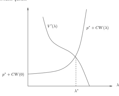
LetF(x, y) be the payoff for a customer who selects strategy xwhen all others select strategyy. Assume that for anyy there exists a unique best responsex(y):
x(y) = arg max
x F(x, y).
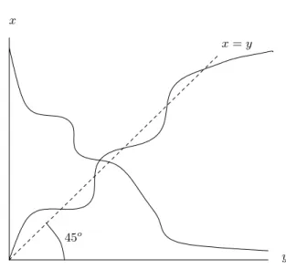
We are interested in cases where x(y) is continuous and strictly mono-tone. Figure 1.1 illustrates a situation where a strategy corresponds to a nonnegative number. It depicts one instance wherex(y) is mono-tone decreasing and another where it is monomono-tone increasing. We call these situations avoid the crowd (ATC) and follow the crowd (FTC), respectively. The rationale behind this terminology is that in an FTC (respectively, ATC) case, the higher the values selected by the others, the higher (respectively, lower) is one’s best response.
Introduction 7
y x=y x
45o
Figure 1.1. ATC and FTC instances
An equilibrium strategy y satisfies x(y) = y. In other words, it is a fixed point of the function x. It is of interest to determine if a model is ATC or FTC since, clearly, in the ATC case at most one equilibrium exists whereas multiple equilibria are possible in the FTC situation.
2.
Threshold strategies
In this section we describe a class of strategies, known as threshold strategies, which is common in queueing systems. Suppose that upon arrival the customer has to choose between two actions,A1andA2, after
observing a nonnegative integer-valued variable which characterizes the state of the system. For example, the state may be the length of the queue and the actions may be to join or to balk.
A pure threshold strategy with threshold n prescribes one of the ac-tions, say A1, for every state in {0,1, . . . , n−1} and the other action,
A2, otherwise.
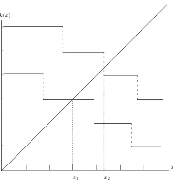
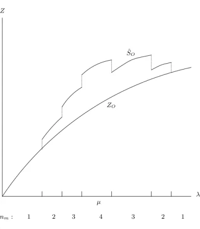
In many cases it is natural to look for an equilibrium pure threshold strategy. However, it is often possible to construct instances where, for example, if everyone in the population uses the threshold 4 then the best response for an individual is 5 and if everyone in the population adopts the threshold 5 then the best response is 4. This is the case with the upper function in Figure 1.2. In such cases, a pure threshold strategy that defines an equilibrium may not exist. Consequently, the definition of a threshold strategy is extended as follows:
8 TO QUEUE OR NOT TO QUEUE A threshold strategy with threshold x = n+p, n ∈ IN , p ∈ [0,1), prescribes mixing between the two pure threshold strategiesnandn+ 1 so that strategynreceives the weight of 1−pand strategyn+ 1 receives the weight ofp. The resulting behavior is that all select a given action, say A1, when the state is 0 ≤ i ≤ n−1; select randomly between A1
andA2 when i=n, assigning probability ptoA1 (the action prescribed
by strategyn+ 1) and probability 1−pto A2 (the action prescribed by
strategyn); selectA2 wheni > n. Ifxis an integer (p= 0), the strategy
ispure. Otherwise, it ismixed.
We are interested in models where a best response for an individual against any strategy x is a pure threshold strategy: for some integer
k(x), if the state is in {0, . . . , k(x)−1} choose A1. Otherwise, choose
A2. The following situation is typical: k(x) has points of discontinuity
with a step of unit size which may be upwards or downwards. At a point of discontinuity x, both of the two pure strategies involved are best responses againstx and hence any mixing between them (which is a mixed threshold strategy) is also a best response againstx. A threshold
xdefines an equilibrium if eitherk(x) =x(in which casexis an integer) orxis between k(x−) andk(x+).2 In both cases, if all customers adopt
the threshold strategyx, then this is also a best response and no one has an incentive to deviate to another strategy. In short, it is an equilibrium strategy.
Recalling from Section 1.6, the behavior reflected by a monotone non-increasing functionk(x) is referred to asavoid the crowd(ATC). It means that the higher is the threshold adopted by others, the lower is the threshold giving the best response for a given customer. Similarly, the case wherek(x) is monotone non-decreasing is referred to asfollow the crowd(FTC). It means that the higher the threshold adopted by others, the higher is the threshold giving the best response for a given customer. There are important differences between the two cases. Under ATC there is at most one fixed point. It may describe a pure strategy or a mixed one. Figure 1.2 depicts two non-increasing step functions. In one, the equilibrium strategy obtained at x1 is pure, in the other, the
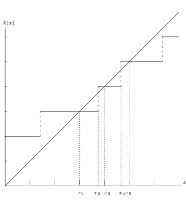
equilibrium strategy obtained at x2, is mixed. The FTC case is more
involved and it may have multiple equilibria. It can be seen from Figure 1.3 thatk(x) may have numerous fixed points.
Remark 1.2 The data are said to be non-degenerate if none of the jumps ofk(x) occur at an integerxvalue. Letx1, x2, . . .be the values of
2It is convenient to view both cases as solutions to the equationk(x) =x, that is, as fixed
Introduction 9
-| | | | | x
k(x)
x2
x1
|
Figure 1.2. Equilibrium in an ATC situation
the fixed points. From Figure 1.3 we observe that fork= 1,2, . . .,x2k+1
corresponds to a pure equilibrium strategy whereasx2kcorresponds to a
mixed equilibrium strategy. When we allow degenerate data there may be consecutive pure equilibrium strategies. If the equilibrium is unique then it is pure.
3.
Costs and objectives
The welfare of a customer consists of benefits associated with service, from which direct payments and indirect costs associated with waiting are subtracted. The sum of direct and indirect costs is referred to as the full price. We assume that the customers involved are risk neutral in the relevant range of payments and benefits so that they maximize their expected welfare.
In most cases it is assumed that the value of a unit of time for each customer is constant (denoted byC), so that spending t time units in
10 TO QUEUE OR NOT TO QUEUE
-| | | x
k(x)
x1 x2 x3 x4x5
| | |
Figure 1.3. Equilibrium in the FTC situation
the system has a total cost ofCt.3 The value of C may differ from one
customer to another.4
A queueing system may also be considered from a social point of view. When we adopt this viewpoint, we assume that the goal in controlling the system is to maximize social welfare which is defined here as the total expected net benefit of the members of the society, including both customers and servers. From this approach, a payment transferred be-tween individuals in the population has a zero net effect on social welfare and thus no effect on the system’s optimization. Therefore, the social goal is to maximize the sum of benefits from service minus waiting and operating costs.
3An interesting generalization to this rule is proposed by Balachandran and Radhakrishnan
[19]. Suppose that waitingttime units costsCeatfor given parameters C >0 anda≥0. Then, the expected waiting cost of a customer isR0∞Ceatw(t)dtwherew(t) is the density function of the waiting time. In anM/M/1 systemw(t) = (µ−λ)e−(µ−λ)t whereλis the arrival rate andµis the service rate. In this case the expected cost equals C
µ−a−λ. Note that the case of linear waiting costs is obtained whena= 0.
4See Deacon and Sonstelie [43] and Png and Reitman [140] for empirical studies concerning
Introduction 11 In some cases we will deal with models of class decision, where cus-tomers belong to classes and each class makes its decisions to maxi-mize the total welfare of its members. This assumption leads to a non-cooperative game with a finite number of players. It is assumed that the arrival processes of customers in various classes are independent, and in particular, if the joint arrival process is Poisson with rateλ, and the pro-portion of class-icustomers ispi, then the arrival process ofi-customers
is Poisson with ratepiλ.
We use the term waiting timefor the time from arrival to departure. Some authors use the termsojourn time. Waiting time excluding service time is referred to asqueueing time.
4.
Queueing theory preliminaries
This section contains a short account of some basic concepts and re-sults from queueing theory which will be used frequently in this book. We use conventional notation to describe basic models. For example, an M/G/s system has s identical servers facing a Poisson stream of customers and no specific service distribution is assumed (M stands for “Markovian” whereas G stands for “general”). The quoted results as-sume steady-state conditions.
We consider a variety of types of decisions made by the customers of a queueing system. A main one is whether to join or not. We apply the common terminology that distinguishes between balking as the act of refusing to join a queue andrenegingas the act of leaving a queue after joining it. The arrival process usually refers to the process by which the demand for service is generated, whereas thejoining processconsists only of those customers who decide to join (i.e., they do not balk). In the literature, the rates of arrival and joining are often termed as the potential demand, and the effective arrival rate. When the arrival and joining rates differ, that is when balking is exercised, we often use Λ for the arrival rate andλfor the joining rate.
The service discipline mostly discussed in this book iscome first-served(FCFS). However, we frequently deal with other regimes. There are two common versions of last-come first-served (LCFS) disciplines. The first, without preemption, in which a new arrival is positioned at the head of the queue but the customer in service is allowed to complete it. The second, with preemption, in which a new arrival preempts a customer who might be in service. It is usually assumed that service, when resumed, is continued from the point where it was interrupted. The acronym used to describe this discipline is LCFS-PR.
Another queueing regime isprocessor sharing. It has two common ver-sions. Underegalitarian processor sharing(EPS) the server splits its
ser-12 TO QUEUE OR NOT TO QUEUE vice capacity evenly among all present customers. In particular, ifn cus-tomers are present during the entire time interval of length ∆t, and at the beginning of this interval their completed workloads were (x1, . . . , xn),
then at its end their completed workloads are (x1+ ∆nt, . . . , xn+ ∆nt).
Also, if the service requirements are exponential with rate µ, then a tagged customer completes his service during the next ∆tunits of time with probability µn∆t+o(∆t). Otherwise, when the split of capacity is based on customers’ parameters, it is called discriminatory processor sharing(DPS). There are also two versions ofrandom order disciplines. In one, whenever a server becomes free, a random customer from the queue is selected to commence service. In the other version, whenever a server completes service, a customer from the queue is randomly cho-sen to be the one to whom this service is granted. We will mention some similarities between EPS and the latter type of the random order discipline.
A service discipline isstrongif the rule by which the next customer to be served is selected does not take into account the actual residual service requirements. It is work-conserving if the server is never idle when the queue is not empty, and a customer whose service was interrupted resumes it from the point of interruption. Under a work-conserving discipline, the total unfinished work at any time is the same as in the corresponding FCFS model.
Examples for disciplines that are strong and work-conserving are FCFS, LCFS, random order, order which is based on customers payments, and EPS.
Service requirements are assumed to be independent and identically distributed. Denote byµ−1 the (common) expected service requirement (i.e.,µis therate of service). For stability, assume that the system’s uti-lization factorρ= λµ is strictly less than 1 (sometimes, when individual optimization leads to stability, this assumption is removed).
The following five results hold when the arrival process is Poisson with rate λ, the service distribution is exponential (an M/M/1 model) with rate µ, and the service discipline is strong and work-conserving. They also hold forM/G/1 models when the service discipline is either EPS or LCFS-PR.
The probability that n (n ≥ 0) customers are in the system (at arbitrary times as well as at arrival times) is
Introduction 13 The expected number of customers in the system is
ρ
1−ρ. (1.3)
The expected waiting time is 1
µ(1−ρ) = 1
µ−λ. (1.4)
The expected length of abusy period, i.e., the expected time from an arrival to an idle server until the server becomes idle again, is5
1
µ(1−ρ). (1.5)
The expected time between a customer’s arrival and the first time the server is idle is
1
µ(1−ρ)2. (1.6)
The following property holds for M/M/1 queues:
The time it takes to reduce the number of customers in the system fromnton−1,n≥1, and the length of a busy period are identically distributed.
For a general service distribution we obtain the M/G/1 model. The Khintchine-Pollaczek (K-P) formula calculates the expected queueing time in an M/G/1 queue where the service discipline is strong, work-conserving and without preemption. Examples for such disciplines are FCFS, LCFS without preemption, and random order. Examples for disciplines for which the K-P formula does not hold are EPS and LCFS-PR. The K-P formula says that the expected queueing time (excluding service) is
Wq=
λx2
2(1−ρ), (1.7)
wherex2 denotes the mean squared service time.
5This expression is identical to (1.4). It can be explained by observing that in a LCFS-PR
M/M/1 system, an arrival stays for a length of time that has the same distribution as a busy period. Moreover, all strong and work-conserving disciplines inM/M/1 queues share the same expected waiting time.
14 TO QUEUE OR NOT TO QUEUE
5.
A shuttle example
In this section we illustrate some of the issues presented in the previous section.6 The model is concerned with two servers operating according to different modes of batch service. For convenience, we present the model in terms of transportation services. Consider two types of such services. The first is a shuttle service that departs whenever the number of waiting passengers reaches the transporter’s capacity.7 We assume the
capacity of a transporter is seven passengers. No limit on the number of transporters is assumed. The second is a bus service. Buses arrive according to a stochastic process with a known expectedresidual inter-arrival time8 which we assume to be five minutes. No limit on the bus capacity is assumed.
Commuters are assumed to have no preference as to the type of ser-vice, and their only concern is their expected waiting times. The gen-eration of commuters who require service is assumed to form a Poisson process with rateλ. We analyze the commuters’ decision process under two different cases. In the observable model, an arriving commuter ob-serves the number of waiting commuters at the shuttle service, whereas in the unobservable model he does not have this information.
5.1.
The unobservable model
Suppose that when making their choice, commuters are not informed about the number of commuters at the shuttle terminal at that instant. Also, once a decision is made, it is too costly to change it.
The waiting time of a commuter who selects the shuttle service de-pends on the choice made by the others. Specifically, the higher the rate of arrival to the shuttle station, the lower the expected waiting time for this service. Thus, if a critical mass of the commuters chooses the shuttle service, then the expected waiting time until the shuttle departs might be sufficiently low, making it attractive for individual commuters. This, of course, is possible only ifλis not too small. We will show that the precise condition is λ > 35, which is assumed below. Consequently, we expect one of the following situations: either all choose the shuttle service, or none do.
6The model which we describe in this section is an example of acoordination game. See, for
example, Crawford [38].
7Compare with Kosten’s “unscheduled ferry problem” and “custodian’s problem” [93]. 8The residual inter-arrival time is the period between a random inspection of the process
Introduction 15 Both solutions define equilibria and nothing in the description of the model can determine which solution will be obtained. Moreover, as we show next, both are ESS.
A strategy, pure or mixed, corresponds to a fraction, p, which is the probability of selecting the shuttle service (so that 1−pis the probability of selecting the bus operation). LetW(p, q) be the expected waiting time for an individual who uses strategy p, while the others use strategy q. Strategy pis an ESS if the following two conditions hold:
W(p, p)≤W(q, p) for any strategy q;
ifW(q, p) =W(p, p) forq =6 p, then W(p, q)< W(q, q).
Both p = 0 and p = 1 are ESS, since W(1,1) < W(q,1) (respectively,
W(0,0) < W(q,0)) for any q 6= 1 (respectively, q 6= 0) and hence the second condition for an ESS is automatically satisfied.9
Next we examine whether additional equilibria, obviously mixed, ex-ist. Suppose that commuters use a mixed (symmetric) strategy with 0< p < 1. The resulting arrival process to the shuttle is Poisson with ratepλ. This strategy defines an equilibrium if commuters are indiffer-ent between using the shuttle and the bus, so that no commuter has an incentive to change his behavior. However, such an equilibrium is not an ESS. Indeed, if any fraction (let alone all) of the commuters changes its behavior, say by making the bus service more popular, this will tip the balance and make the bus service more attractive. In other words, deviation from the equilibrium is self-perpetuating, and it causes more (and more) to deviate in the same direction, leading to a new equilib-rium in which all use the bus. Similarly, any shift to a more frequent use of the shuttle service will result in everybody using this service.
Recall that the shuttle capacity is 7 and the expected waiting time for a bus is 5 minutes. Assume that the commuters follow the mixed strategy
p. If a tagged commuter selects the shuttle service, then the number of waiting commuters that he meets upon arrival is i with probability 17 fori= 0, . . . ,6, and his expected waiting time equals 6λp−i.10 Therefore, his (unconditional) expected waiting time is λp3 . Ifp < 53λ (respectively,
p > 53λ) then his unique best selection is the bus (respectively, shuttle).
9If, for example, the shuttle operator prefers the solution withp= 1, then one way to attain
this goal is by convincing the commuters that this is indeed the situation!
10This is where the steady-state assumption is used. The number of commuters waiting for
the shuttle service defines a Markov process with the state spaceS={0,1, . . . ,6}. The only transitions are from stateito state (i+ 1)mod6 and they all have ratesλp. The resulting limit probabilities are uniform.
16 TO QUEUE OR NOT TO QUEUE
45o
1 1
Best response
p pe
Figure 1.4. Best response vs. fraction of shuttle users
He is indifferent between the two options if p = pe where pe = 53λ.11
Thus, pe is an equilibrium strategy. However, pe is not an ESS. For
example, W(0, pe) =W(pe, pe) butW(0,0)< W(pe,0) =∞. A similar
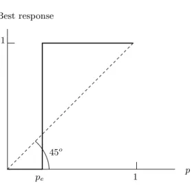
result holds when 0 is replaced with 1. In fact,pe is a best response for
an individual only if all others use this strategy, whereas any strategy
p is a best response against pe. Note that if all use p > pe then 1 is
uniquely the best response, and if p < pe then 0 is uniquely the best
response (see Figure 1.4).
Remark 1.3 The best response function is monotone non-decreasing. This is an example of an FTC situation, which explains the existence of multiple equilibria.
To summarize, three equilibrium strategies exist in the non-trivial case where λ > 35. The two pure equilibria are ESS. Moreover, p = 0 remains the unique best response as long as the rest use strategy
p < 53λ. Similarly, p = 1 is the unique best response as long as the the rest use strategy p > 53λ. The stability of the equilibria p = 0 and p = 1 is reflected by the property that even if a non-negligible deviation from strategies 0 or 1 takes place among all commuters, the best response is not affected. The mixed equilibrium prescribes the shuttle with probabilitype= 53λ. This equilibrium is not an ESS.
11When 3
5λ >1, commuters appear at a rate so low that even when all of them use the shuttle service, the individual’s best response is still to use the bus service. In other words, whenλ <35, using the bus service is a dominant strategy.
Introduction 17
5.2.
The observable model
Assume now that commuters observe the number of people already waiting at the shuttle terminal, and then decide which service to choose. Of course, the higher the number of commuters already waiting for the shuttle, the more a new arrival tends to select this service.
Consider an individual who arrives when the shuttle is empty, and assume the most favorable case in which all select this service. His expected waiting time for the shuttle service is then λ6. If under these conditions it is best for him to select the shuttle service, it is of course also best for those who observe a longer queue for the shuttle service. On the other hand, if he does not select the shuttle service, nobody will (the next arrivals will also face an empty queue and will follow through with the same reasoning), and hence this service will never be used. The conclusion of this analysis is that if λ > 65, all use the shuttle service and ifλ < 65, none do.
This informal analysis is correct but not complete. In particular, it does not distinguish between equilibria which are subgame perfect and those which are not. We now proceed with a formal analysis.
A pure strategy is a function from the number,i, of commuters wait-ing for the shuttle upon arrival of a commuter to the set of actions (i.e., which service to select). For example, the strategyδ = (s, b, s, b, s, b, s) prescribes taking the shuttle wheneveriis even and taking the bus when-ever i is odd. It is clear that those states where b is prescribed are recurrent (in fact, absorbing) and those wheres is prescribed are tran-sient. The exception for the latter isδ= (s, s, . . . , s) where all states are recurrent.12
When λ > 65, (s, s, . . . , s) is the unique equilibrium. Moreover, as all states are recurrent this is also the unique SPE. The analysis is more involved whenλ < 65. Now the strategy (s, s, . . . , s) is not an equilibrium: given that all follow it, it prescribes a suboptimal action for the recurrent statei= 0. Therefore, a necessary condition for a pure strategyδ to be an equilibrium is thati(δ)≥0 where
i(δ) = max{i|δ(i) =b}.
As said above, all states for which the bus is prescribed under δ are recurrent (in fact, absorbing), whereas the others are transient. Thus, for
12A state is said to berecurrentif a Markov process which initiates in it will visit it again
with probability 1. Alternatively, this state will be visited an infinite number of times with probability 1. A recurrent state is said to be absorbingif once a process enters it, it will stay there forever with probability 1. A non-recurrent state is said to betransient. In other words, a Markov process which initiates in it will visit it again with probability less than 1, and thus the number of visits there is finite with probability 1.
18 TO QUEUE OR NOT TO QUEUE an equilibrium, only optimality at the former group has to be checked.13
In fact, only optimality ati(δ) has to be checked since ifbis an optimal action at i(δ), it is certainly an optimal action for states i such that
i < i(δ), and if δ(i) = s for i6= i(δ) then i is transient. In particular,
δ is an equilibrium if and only if 6−λi(δ) ≥5. In other words, the set of pure equilibria are allδ with 0≤i(δ)≤6−5λ.
Clearly, in a SPE, sis prescribed for state 6. Given that i >6−5λ
and that for every state j, j > i, the strategy prescribes s, then to be a best response, the strategy must also prescribesto statei. Likewise, for statesi≤6−5λit must prescribeb. Thus, an equilibrium strategy is subgame prefect if and only if it prescribes the bus for all states
i≤6−5λand the shuttle for the rest.
To summarize, excluding the cases where 6−5λis an integer, for any
λ there exists a unique SPE which is of the type (b, . . . , b, s, . . . , s).14 When 6 −5λ ≥ 2, more equilibria exist and they are of the form (x, . . . , x, b, s, . . . , s) where x stands for any action and the last b ap-pears in some positioni wherei≤6−5λ.
We conclude the equilibrium analysis by comparing the unobservable and the observable cases. When 35 < λ < 65, the shuttle operator is better-off in the unobservable case than in the observable case. Indeed, in the unobservable case, there is one ESS in which the shuttle operator gets all of the demand whereas in the observable case, the shuttle op-erator gets no demand at all in all possible equilibria. If the option is given, the shuttle operator would conceal the information on how many commuters are waiting. The opposite holds whenλ > 65. Here, when the information is concealed there exists an ESS where the shuttle operator receives no demand. Therefore, the shuttle operator prefers to reveal the information and get all the demand in the unique equilibrium (in fact, SPE).15 When λ < 3
5, the shuttle operator is indifferent between the
options since in both cases all of the demand goes to the bus operator.
5.3.
Social optimality
We now illustrate the difference between the equilibrium solution and the solution that maximizes the overall welfare of the commuters. In our model, a commuter who chooses the shuttle generatespositive external-ities. This means that by increasing the rate of arrival to the shuttle, the expected waiting time of the other commuters who make the same
13The steady-state assumption is used here: under these conditions, the transient states have
zero probability of being observed by an arrival.
14The set ofb’s may be empty, whenλ >6
5, but not the set ofs’s. 15Compare with§3.2.
Introduction 19 choice is reduced (whereas the expected waiting time of the bus users is not affected). Customers who independently maximize their own welfare ignore these externalities, and it therefore may happen that the shut-tle is less used in equilibrium than under a social welfare maximizing solution.
The socially optimal solution of the unobservable model is simple. Since the social goal is to minimize the expected waiting time, the solu-tion is either that all commuters use the shuttle or that they all use the bus. In the first case the expected waiting time is 3λ and in the second case it is 5. Therefore, if λ > 35 then all should use the shuttle, and if
λ < 35 then all should use the bus. Ifλ= 35 the two solutions are socially equal, meaning that it does not matter which means of transportation the commuters use, as long as they all use the same one. Note that when
λ < 35 the unique equilibrium solution is socially optimal. When λ > 35, social optimality requires that all use the shuttle, but the solution that all use the bus is also an equilibrium.
The social considerations in the observable case are similar to those in the unobservable case, and the same behavior is optimal: if λ > 35
then all should use the shuttle, and ifλ < 35 then all should use the bus. Note that when λ > 65, the socially optimal solution where all use the shuttle is also an equilibrium, but in the range 35 < λ < 65 the socially optimal solution where all use the shuttle is not an equilibrium. The reason, as we have mentioned before, is that the commuters ignore the positive externalities associated with the action of choosing the shuttle. Among those who ignore the externalities are those who arrive to an empty shuttle: optimizing their individual welfare they prefer the bus but socially it is desired that they join the shuttle’s queue.
6.
Non-stochastic models
In this section we briefly mention some papers that deal with equi-libria in non-stochastic queueing models. When a good is available in limited quantity and sells below market price, queues form. The length of waiting time stabilizes at such a level that the full price (consisting of the good’s nominal price plus the waiting cost) of the marginal potential consumer equals the good’s value. Thus, the resulting equilibrium wait-ing time may be independent of the service time. Barzel [26] explained that
the resource cost of this allocation, time spent in the queue, represents a cost of establishing property rights in the good.
20 TO QUEUE OR NOT TO QUEUE He also concluded that although one expects the poor, who have low time value, to profit from the institution of “rationing by waiting”, the beneficiaries may often be among the rich.
Donaldson and Eaton [46] considered price discrimination between consumers with low and high time values by offering to sell the product under two options involving different combinations of money and time prices. We will describe related queueing models in§7.
Another model in Shy [156], is based on MacKie-Mason and Varian [115]. There, the utility of customer i, i = 1, . . . , n, is assumed to be given by
Ui =√qi−C
Q U −pqi,
where qi is the capacity allocated to (or used by) customer i, Q =
Pn
j=1qj,U is the total capacity available, C is a cost parameter, and p
is a price charged per unit of capacity. The term CQU reflects the effect of congestion. Shy derived the equilibrium as well as the social optimal capacity allocations, and showed that the two coincide whenp=CnU−1. Several other papers in the economic literature deal with rationing of goods through queueing, see [6, 135, 141, 160] and their references. These papers model centrally planned economies in which products can be purchased at a low official price after waiting in queues. The products can also be purchased in “black markets” at higher prices and without waiting. This situation opens possibilities for poor customers to spend their time in queues, buy products at the official prices, and re-sell them in the black market. Thus, each individual allocates his resources, money and time, in order to maximize his utility. This literature treats waiting times in queues in the same way it treats the prices, namely, it searches for prices and waiting times which determine equilibria, and apart from this no queueing mechanism that relates waiting time to supply and demand is assumed. Therefore, such models do not fit the framework of this book.
Chapter 2
OBSERVABLE QUEUES
This chapter deals with queueing systems, where an arriving customer observes the length of the queue before making his decisions.
1.
Naor’s model
The subject of Naor’s paper [133] is the control of a FCFS M/M/1 system. In Naor’s model, a queue manager announces an admission fee, and customers react by setting a pure strategy which distinguishes the states of the queue where customers join from those where they balk. It is easily seen that individual optimization generally determines an equilibrium based on a pure threshold strategy. The concept of equilib-rium is not central in this model since the decision of whether to join the queue in a given state is independent of the strategy adopted by the other customers. Yet, a customer’s decision to balk when observing a queue length greater than the threshold, is based on the assumption that those present in the queue will not leave (renege) before they are served (see Remark 2.1 below).
Naor noticed that in observable queues the individual’s decision devi-ates from the socially preferred one. This gap is caused by externalities generated when joining the queue: a customer who joins the queue may cause future customers to spend more time in the system. The indi-vidual’s objective does not take these externalities into consideration. Because of these negative external effects, the equilibrium arrival rate is
22 TO QUEUE OR NOT TO QUEUE greater than the socially desired one.1 We start by listing the
assump-tions underlying Naor’s model:
1 A stationary Poisson stream of customers - with parameterλ- arrives to a single server facility.
2 The service times are independent, identically, and exponentially dis-tributed with parameterµ.
3 A customer’s benefit from completed service isR.
4 The cost to a customer for staying in the system (either while waiting or while being served) isCper unit of time.
5 Customers are risk neutral, that is, they maximize the expected value of their net benefit.
6 Utility functions of individual customers are identical and additive, from the public (social) point of view.
7 Rµ≥C.2
8 The service discipline is FCFS.
9 A decision to join is irrevocable, and reneging is not allowed.
10 Upon arrival, a customer inspects the queue length and decides whether to join or balk. A customer who balks leaves the system and never returns.
The individual’s optimizing strategy in this model is straightforward. A customer who joins the queue when i customers are already in the system (including the one who is currently served) expects a benefit
R−(i+1)µC. The customer then enters if this value is nonnegative, that is, ifi+ 1≤ RµC . Otherwise, the customer balks. Consequently, the pure threshold strategyne with3
ne=
Rµ
C
, (2.1)
is an equilibrium strategy. Under this strategy, an arriving customer joins the queue if he observesne−1 or fewer customers and balks if he
observes ne customers or more. Note that ne is the maximum possible
number of customers in the system under individual optimization, and the result is anM/M/1/ne queueing system.
Overall (social) optimization is not as trivial. We observe that there exists a pure threshold socially optimal strategy. This can be argued as
1Individual optimization causes more congestion than is socially desired also in more general
models. See, for example, Mills [129].
2Otherwise, all individuals, even in the most ideal situation of observing an empty system,
would balk.
Observable queues 23 follows: clearly, a pure optimal strategy exists, and any pure strategy is in effect a threshold strategy, where the threshold coincides with the smallest queue size for which the strategy prescribes balking (see Remark 2.2).
Denote by SO the expected social benefit per unit of time.4 Given a
maximum queue length of n, the probability of observing n customers in the system isqn= ρ
n
Pn i=0ρ
i. Assuming ρ6= 1, the probability that an
arriving customer joins is5
1−qn=
1−ρn
1−ρn+1, (2.2)
and the expected number of customers in the system is
Ln=
ρ
1−ρ −
(n+ 1)ρn+1
1−ρn+1 .
Hence,
SO = λR(1−qn)−CLn
= λR 1−ρ
n
1−ρn+1 −C
"
ρ
1−ρ−
(n+ 1)ρn+1
1−ρn+1
#
. (2.3)
Let n∗ be a maximizer of (2.3). Naor designed a procedure for com-putingn∗ which is based on the property that the function given in (2.3) is unimodal.6 Naor also showed that n∗ ≤ ne. In the next section we
present an alternative derivation forn∗.
In order to motivate customers to adopt the thresholdn∗ rather than
ne, Naor suggested imposing an appropriate admission fee. Based on
(2.1), an admission feepinduces the socially optimal threshold if
n∗= (R
−p)µ C
. (2.4)
Payments are not considered part of the social welfare function and therefore the exact fee is irrelevant as long as it satisfies (2.4).
Alternatively, the queue can be regulated by imposing a toll on wait-ing, i.e., increasing C instead of reducingR. Such a toll, t, induces the
4The subscriptOstands forobservable.
5The results hold also forρ= 1 when taking the appropriate limits. In fact, in this case
1−qn=nn+1.
24 TO QUEUE OR NOT TO QUEUE optimal threshold n∗ if
n∗ =
Rµ
C+t
.
We will deriven∗ in Section 3.
Remark 2.1 If Assumption 9 is relaxed and customers are allowed to renege, the decision of whether or not to join may depend on the behavior of the customers who are already in the system. If some of them plan to renege, then a customer may join even if he observes ne or more
customers in the queue. Yet, for a customer who joined after observing at mostne−1 customers, reneging later is clearly a suboptimal action
(see§5.1). After eliminating strategies that prescribe reneging, it is best for an arriving customer who observesne to balk.
Remark 2.2 Unless Rµ
C is an integer, the unique threshold equilibrium
strategy is ne. However, there are other non-threshold equilibria. For
example, joining whenever the queue size is not ne, is an equilibrium.
This may seem puzzling at first, but if all follow this strategy, then the states corresponding to ne+ 1 customers or more are transient. Hence,
whatever is prescribed for these states is irrelevant to establishing (or refuting) that a strategy defines an equilibrium. It is true, though, that the threshold strategyne is the unique SPE.
Remark 2.3 If Rµ
C is an integer, then mixing with any probability
be-tween joining and balking when observingne−1 customers (and
other-wise doing as before) is also an equilibrium strategy.
2.
The LCFS-PR model
Hassin [65] suggested a way to achieve social optimality without im-posing admission fees. This section is devoted to describing this ap-proach and its implications. We adopt Naor’s model with two changes:
Assumption 8 changes as follows:
The service discipline is LCFS-PR, that is, a newly arrived customer joins the system and is immediately served, possibly preempting the service of another customer. Preempted customers join a queue where later arrivals get priority over earlier arrivals. When a preempted customer’s turn to re-enter service comes, his service is resumed from the point of interruption.
Assumption 9 changes as follows:
At any instant, each customer is allowed to renege at no additional cost and never return. The queue is fully observable at any instant, so that a customer can base his decision on the queue length and on his position in it.
Observable queues 25 In a FCFS queue, a new customer is placed at the end of the queue, and therefore imposes no negative externalities on customers already in the system. However, this customer may impose negative externalities on future arrivals. The essence of the discrepancy between individual and social optimization in Naor’s FCFS model lies in the fact that the customer ignores these externalities. Therefore, the individual may join a queue even when his own expected welfare is smaller than the expected reduction in welfare to future customers.
The externalities imposed by a newly arrived customer on those who are presently in the system, are highest if he is assigned to the head of the queue. Under LCFS-PR, every arriving customer is placed at the head of the queue, pushing back those customers who arrived earlier. However, all future arrivals will be placed in front of him and therefore he does not impose any external effects on them.
Hassin observed that LCFS-PR leads to a socially optimal behavior by the customers. The relevant decision that an individual faces iswhen to leave the queue rather than whether to join it. By the memoryless property of the exponential distribution it follows that the distributions of the customers’ residual service are independent of the queue length and of the amount of service each of them has already received. Since the model assumes homogeneous customers, the waiting customers have identical time and service values as well as identical distributions of residual service time. Therefore, when a customer decides to renege there is no other customer behind him. Since everybody present is served prior to the person at the end of the queue, he imposes no externalities, regardless of his action. In other words, his considerations coincide with those of the society, and hence he will reach the same conclusion of whether or not to renege. In particular, his threshold isn∗. (Note that from the social point of view the order of service is irrelevant, so that the socially optimal threshold is the same under the FCFS and LCFS-PR regimes.) In the next section we use this observation in order to determinen∗.7
We now discuss the LCFS-PR model and its implications.
There is a strategic difficulty associated with the LCFS-PR model. A customer whose service has been preempted is motivated to renege and re-enter the system, pretending to be a new arrival. Such
behav-7Remarks 2.1 and 2.2 also apply to the FCFS-PR model. A customer in positionn∗knows
that the same reasoning that led him not to renege earlier leads everyone in front of him not to renege while in positions 1 ton∗−1. Similarly, the equilibrium is not unique. For
example, reneging if and only if there are exactlyn∗customers ahead in the queue is also an
26 TO QUEUE OR NOT TO QUEUE ior contradicts Assumption 10 in Naor’s model and therefore must be prevented administratively.8
The important property of the LCFS-PR model that leads to optimal individual behavior is that the last customer in the queue remains at the end of the queue as long as he is in the system and therefore he imposes no externalities. This property is preserved by any queue discipline with the property that the newly arrived customer is placed anywhere except for at the end of the queue. A particularly appeal-ing policy is to assign a newly arrived customer, whenever the server is busy, to the position before the last. This policy reduces the cus-tomer’s incentive to renege and re-enter as a new arrival. There is, however, another difficulty associated with this solution. Suppose that customer A is now at the end of the queue while B is just one position ahead of him. If A reneges, then B becomes the last one, and all future arrivals will be positioned ahead of him. Thus B may find it beneficial to offer A a payment so that A doesn’t renege. Such side payments must be prevented to preserve optimal behavior. This can be done by concealing the identities of the customers in the queue. The solution just proposed has other advantages over LCFS-PR: (i) Preemption may incur some loss of service and this solution is asso-ciated with fewer preemptions. (ii) Risk averse customers are worse off under the LCFS-PR discipline than under other queue disciplines like FCFS, since LCFS-PR is associated with a larger waiting time variance.9 Under the LCFS-PR rule some customers are continuously
served without waiting while others wait for long periods of time and finally renege without being served. In particular, in a FCFS queue no customer incurs negative utility (assuming that the utility asso-ciated with immediate balking is 0), while this is not the case with LCFS-PR. Assigning new arrivals to the position before last reduces all these drawbacks while maintaining a socially optimal behavior. The model is of course a simplified one. However, the qualitative implications are quite general. It is well known that if customers differ by their characteristics (waiting cost, service distribution, ser-vice value, etc.) social welfare can be increased by proper assignment
8If waiting “at home” is less costly than waiting in the queue it may be socially desirable
that a customer returns to the system after balking or reneging. Models with retrials are discussed in§5.
9Kingman [87] showed that FCFS (respectively, LCFS-PR) minimizes (respectively,
Observable queues 27 of priorities (this is the subject of §4). A consequence of the above discussion is that:
– Assigning priorities may be beneficial even when the customers are identical!
Suppose that priorities are assigned randomly or according to some irrelevant basis. The customer at the end of the queue will usually have low priority, and may expect most future arrivals to be placed in front of him. This decreases the externalities he imposes and makes his decision of whether to renege closer to the socially optimal one. Olson [136] showed that a LCFS-PR regime can be induced through an appropriate price menu, so that customers receive priority levels based on the amount they paid rather than administratively. Such a pricing system will also achieve social optimality. See also§4.1.3. An LCFS-PR discipline induces optimal customers’ behavior also in more general observable models. For example, consider an M/M/s
system, where the servers may have different service rates. An ar-riving customer starts service at the fastest server. This action may preempt the service of an earlier customer who is then moved to the second fastest server, and so on. A customer at the slowest server may be returned to the queue. It is also possible that the customer at the end of the queue reneges at this stage as a result of the increase in his expected waiting time. As in the single server system (and because of the same reasons), reneging is done in the socially optimal way. Variations of this model with s= 2 were analyzed by Xu [177]. Illustrative descriptions of the LCFS-PR model and its consequences were given by Nalebuff in [132] and Landsburg in [98].
3.
Social optimization
In this section we derive the threshold equilibrium strategy under the LCFS-PR regime.10 As discussed in the previous section, this threshold
coincides withn∗, the socially optimal threshold.
Let n be the maximum possible length of the queue, i.e., a customer reneges whenever there are n other customers in front of him. This number includes the one in service. Let fn be the expected benefit for
a customer in positionnin the LCFS-PR queue when all (including the customer under consideration) renege from positionn+ 1. Of course,fn