Bianchi Type- I Viscous Fluid Accelerating Cosmological Models with Time Dependent Q and Λ - Term

ISSN: 2231-5373

http://www.ijmttjournal.org

Page 185

Bianchi Type- I Viscous Fluid Accelerating

Cosmological Models with Time Dependent

Q

and  - Term

Dinkar Singh Chauhan1, R.S. Singh2 ,Anirudh Pradhan3

1,2

Department of Mathematics, Post Graduate College, Ghazipur-233001, India

3

Department of Mathematics, Hindu Post Graduate College, Zamania-232331 (Ghazipur), India

Abstract :

In present paper, exact solutions of Einstein's field equations are obtained in a spatially homogenous and anisotropic Bianchi type-I space-time in presence of a dissipative fluid with constant and time dependent cosmological term. Einstein's field equations are solved by considering a scale factor a

 

t  tet which yields a time dependent deceleration parameter that affords a late time acceleration in the universe. The cosmological constant () is found to be a decreasing function of time and it approaches a small positive value at the present epoch which is corroborated by consequences from recent supernova Ia observations. To get the deterministic solution a barotropic equation of state together with the shear viscosity is proportional to expansion scalar, is also assumed. The physical and geometric properties of cosmological models are also discussed.

Keywords and Phrases :Bianchi type-I universe, variable deceleration parameters, Dissipative fluid.

1. Introduction and Motivation :

The cosmological constant () was introduced by Einstein in 1917 as the universal repulsion to make the Universe static in accordance with generally accepted picture of that time. In absence of matter described by the stress energy tensor Tij,  must be constant, since the Bianchi identities guarantee vanishing covariant

divergence of the Einstein tensor, G_;ij_j  0, while g_;ij_j  0 by definition. If Hubble parameter and age of the universe as measured from high red-shift would be found to satisfy the bound H₀t₀ 1 (index zero labels values today), it would require a term in the expansion rate equation that acts as a cosmological constant. Therefore the definitive measurement of H₀t₀ 1 and wide range of observations would necessitate a non-zero cosmological constant today or the abandonment of the standard big bang cosmology [1]. However, a constant , as it was originally introduced by Einstein in 1917, cannot explain why the calculated value of vacuum energy density at Plank epoch following quantum field theory is 123 orders of magnitude larger than its value as observed or as predicted by standard cosmology at the present epoch [2]. In attempt to solve this problem, variable  was introduced such that  was larger in the early universe and then decayed with the evolution [?]. The idea that  might be variable has been studied for more than two decades [3] ,[ 4] and references therein. Linde [5] has suggested that  is a function of temperature and is related to the process of broken symmetries. Therefore, it could be a function of time in a spatially homogeneous, expanding universe [4]. In a paper on -variability, Overduin and Cooperstock [6] suggested that gij is shifted onto the right-hand side of the Einstein field equation and treated as part of the matter content. In general relativity,  can be regarded as a measure of the energy density of the vacuum and can in principle lead to the avoidance of the big bang singularity that is characterized of other FRW models. However, simplistic properties of the vacuum that follows from the usual form of Einstein equations can be made more realistic if that theory is extended and includes a variable . Recently, Overduin [7],[ 8] has given an account of variable -models that have a non-singular origin. Liu and Wesson [9] have studied universe models with variable cosmological constant. Podariu and Ratra [10] have examined the consequences of incorporating constraints from recent measurements of the Hubble parameter and the age of the universe in the constant and time-variable cosmological constant models. In recent time the -term has interested theoreticians and observers for varied reasons.

ISSN: 2231-5373

http://www.ijmttjournal.org

Page 186

term would expand faster with time because of the push from the cosmological term [11]. In the absence of any interaction with matter or radiation, the cosmological constant remains a ''constant". However, in the presence of interactions with matter or radiation, a solution of Einstein equations and the assumed equation of covariant conservation of stress-energy with a time-varying  can be found. Peebles and Ratra [12] described a cosmology based a -like term that decreases with time because the potential energy of the inflation field  has a power-law tail at large  . Here the mass density , associated with  would act like a cosmological constant that decreases with time less rapidly than the mass densities of matter and radiation. Time-dependent

-like terms have been discussed by Dolgove [?], Banks [13], and references therein for the purpose of obtaining a small value of  from the quantum field theory. The spectrum of fluctuations in the Cosmic Microwave Background (CMB) [14], baryon oscillations [15] and other astrophysical data, indicating that the expansion of the universe is currently accelerating. The energy budget of the universe seems to be dominated at the present epoch by a mysterious dark energy component, but the precise nature of this energy is still unknown. Many theoretical models offer possible explanations for the dark energy, ranging from a cosmological term [16] to super-horizon perturbations [17], [18] and time-varying quintessence scenarios [19]. These recent observations strongly favour a significant and a positive value of  with magnitude 



Gh /c3



10 123 . A.G. Riess et al. [20], [21] have recently presented an analysis of 156 SNe including a few at z 1.3 from the Hubble Space Telescope (HST) "GOOD ACS" Treasury survey. They conclude to the evidence for present acceleration q₀  0



q₀  0.7



. Observations [20]-[22] of Type la Supernovae (SNe) allow us to probe the expansion history of the universe leading to the conclusion that the expansion of the universe is accelerating.

Anisotropic cosmological models play significant role in understanding the behaviour of the universe at its early stages of evolution. Observations by the Differential Radiometers on NASA's Cosmic Background Explorer registered anisotropy in various angle scales. The simplest of anisotropic models, which, completely describe the anisotropic effects, are Bianchi type-I (BI) homogeneous models whose spatial sections are flat but the expansion or contraction rate is directional dependent. The advantages of these anisotropic models are that they have a significant role in the description of the evolution of the early phase of the universe and they help in finding more general cosmological models than the isotropic FEW models. The isotropy of the present-day universe makes the BI model a prime candidate for studying the possible effects of an anisotropy in the early universe on modern-day data observations. Recently, Kalita et al. [23], Dey et al. [24], Oli [25] and Nourinezhad & Mehdipour [26] have studied cosmological models in anisotropic Bianchi type space-times in different context.

Motivated by the above discussions, in this Paper, we have investigated a new class of spatially homogeneous and anisotropic Bianchi type-I cosmological models with time dependent deceleration parameter and cosmological constant in presence of a dissipativc fluid. The Einstein's field equations are solved explicitly. The outline of the paper is as follows: In Sect. 2, the basic equations are described. Section 3 deals with the solutions of the field equations by considering time dependent deceleration parameter. Section 4 describes results and discussions. In Subsect. 4.1, we obtain the solution with variable -term and constant  . Subsection 4.2 deals with the models with variable -term and   . In Subsect. 4.3, we describe the solution with constant -term and time dependent  . Finally, conclusions are given in the last Sect. 5.

2. The Metric and Basic Equations

We consider a spatially homogeneous and anisotropic Bianchi type-I metric in the form

 

2 2

 

2 2

 

2,

2 2 2

dz t C dy t B dx t A dt

ds      (1)

where the metric potentials A, B and C are functions of cosmic time t alone. This ensures that the model is spatially homogeneous.

We define the following parameters to be used in solving Einstein's field equations for the metric (1).

The average scale factor a of Bianchi type-I model (1) is defined as





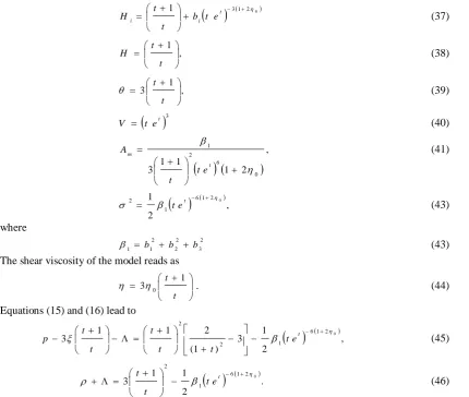
3.

1

ABC

a  (2)

A volume scale factor V is given by

ABC a

V  3  (3)

ISSN: 2231-5373

http://www.ijmttjournal.org

Page 187

            C C B B A A a a H     3 1 (4) , 2 2 aH a a a a

q 

       (5)

where an over dot denotes derivative with respect to the cosmic time t. Also we have



,

3 1

3 2

1 H H

H

H    (6)

where B B H A A H     ₂

1 , and

C C H





3 are directional Hubble factors in the directions of x,y and 

z axes respectively.

The Einstein's field equations (in gravitational unit 8G  c 1) are given by

, 2

1

ij ij

ij Rg T

R    (7)

where Tij is the stress energy tensor of matter which, in case of viscous fluid and cosmological constant, has the form [27]

, ) ( )

( _{i j ij ij ij}

ij p uu pg t g

T       

(8) with





H

p u p

p   i_i 3 2 3 2 ;             (9) and . ; ; ; ;    

_{i j} u_ji u_iu u_j u_ju u_i (10)

In the above equations,  and  stand for the bulk and shear viscosity coefficients respectively;  is

the matter density; p is the isotropic pressure and ui is the four-velocity vector satisfying uiu_i  1.

In a co-moving coordinate system, where ui  ₀i, the field equations (7), for the anisotropic Bianchi type-I space-time (1) and viscous fluid distribution (8), yield

,

2  

     A A p BC C B C C B

B    

 (11)

,

2  

     B B p CA A C A A C

C   

 (12)

,

2  

     C C p AB B A B B A

A    

 (13) .       CA A C BC C B AB B

A    

(14)

Here, and also in what follows, a dot designates ordinary differentiation with respect to t. Equations (11) - (14) can also be written as



2 1



2.

2 _

     

 H q

p (15)

,

3 2  2

    H  (16)

where  is shear scalar given by

ISSN: 2231-5373

http://www.ijmttjournal.org

Page 188

where









. 3 1 2 1 ; ;

; i ij i j

k k j j k k i j i

ij u  u u u u u u   g uu

 (18)

The expansion scalar

 

 and the anisotropy parameter (Am)are defined as

a a u_;i_i  3

  (19)



         3 1 2 . 3 1 i i m H H H

A (20)

The energy conservation equation ;j  0,

ij

T leads to the following expression:







  



 

 2 2

4

  

 p . (21)

It follows from (21) that for contraction, that is,   0, we have   0 so that the matter density increases or decreases depending on whether the viscous heating is greater or less than the cooling due to expansion.

The Raychaudhuri equation is obtained as









2 .

3 1 3

2

1 _{2 2}

           

 p (22)

We have a system of four independent equations (11) – (14) and eight unknown variables, namely   , , , , ,

,B C p

A and . So for complete determinacy of the system, we need four appropriate relations among these variables that we shall consider in the following section and solve the field equations.

3. Solutions of field equations

We follow the approach of Saha [28] and Saha & Rikhvitsky [29] to solve the field equations (11) – (14). Subtracting (11) from (12), (11) from (13), (12) from (13) and taking second integral of each, we get the following three relations

, exp 2 3 1 1        

_

  dt e a x d B

A dt

(23) , exp 2 3 2 2        

_

  dt e a x d C

A dt

(24) , exp 2 3 3 3        

_

  dt e a x d C

B dt

(25)

where d1,x1, d2,x2, d3 and x3 are constants of integration.

From (23) – (25), the metric functions can be explicitly written as

 

exp ,

2 3 1 1       

 a a b

_

a e dt

t A

dt 

(26)

 

exp ,

2 3 2 2        

_

  dt e a b a a t B dt  (27)

 

exp ,

2 3 3 3        

_

  dt e a b a a t C dt  (28) where





, ,

, 3 1

3 2 3 3 3 1 1 2 3 2 1 1    

 d d a d d a d d

a





. 3 , 3 , 3 3 2 3 1 3 2 2 1 1 x x b x x b x x

b       

These constants satisfy the following two relations

. 0 ,

1 _{1 2 3}

3 2

1a a  b b  b 

a (29)

ISSN: 2231-5373

http://www.ijmttjournal.org

Page 189

For any physically relevant model, the Hubble parameter and deceleration parameter (DP) are the most important observational quantities. The first quantity sets the present time scale of the expansion while the second one reveals that the present state of evolution of universe is speeding up instead of slowing down as expected before the type Ia supernovac observations [30]-[32]. We consider the variation of scale factor a with cosmic time t by the relation

 

t t et,

a  (30)

The relation (30) has been used by Pradhan et al. [36] in studying some Bianchi type-I cosmological models in scalar-tensor theory of gravitation with time dependent deceleration parameter.

From (5) and (30), we get the time varying DP as

 



1



1.

1

2   

t t

q (31)

The motivation to choose such time dependent DP is behind the fact that the universe is accelerated expansion at present as observed in recent observations of Type la supernova [31], [32], [20]] and CMB anisotropics [33]-[35] and decelerated expansion in the past. Also, the transition red shift from deceleration expansion to accelerated expansion is about 0.5. Now for a Universe which was decelerating in past and accelerating at the present time, the DP must show signature flipping [37], [ 38]. So, in general, the DP is not a constant but time variable.

It is worth mentioned here that the choice of a(t) given by Eq. (30) yields a time-dependent DP (31) which generates an accelerating phase in the expansion of universe at present epoch.

Next, we assume that the coefficient of shear viscosity (0) is proportional to the expansion scalar

 

 i.e.

,



  which leads to

 

  ₀ (32)

where 0 is proportionality constant. Such relation has already been proposed in the physical literature as a

physically plausible relation [39],[ 40].

Finally to conveniently specify the source, we assume the perfect gas equation of state, which may be written as

1 0

,  

 

p (33)

Using Eqs. (19),(30) and (32) into (26) – (28), we get the following expressions for the scale factors  

], )

( [ exp )

( 31 2 0

1

1



 

 a te b te dt

A t t  (34)

 

], )

( [ exp )

( 31 2 0

2

2



 

 a te b te dt

B t t  (35)

 

], )

( [ exp )

( 31 2 0

3

3



 

 a te b te dt

ISSN: 2231-5373

http://www.ijmttjournal.org

Page 190

Figure 1: The plot of anisotropy parameter Amversus t for 0  0.1

4. Some Physical and Geometric Properties of three Models

The physical parameters such as directional Hubble factors (Hi), Hubble parameter (H), expansion scalar ( ),

spatial volume (V), deceleration parameter (q), anisotropy parameter (Am)and shear scalar ()are given by

 

31 2 0

1   

       

 t

i

i b t e

t t

H (37)

, 1

       

t t

H (38)

, 1

3 

      

t t

 (39)

 

_t 3

e t

V  (40)

 





,

2 1 1

1

3 ₀

6 2

1

 

 

      

t m

e t t

A (41)

 

 

, 2

1 61 2 0

1

2 _ 

  t  

e

t (43)

where

2 3 2 2 2 1

1  b  b  b

 (43)

The shear viscosity of the model reads as

       

t t 1 3₀

 . (44)

Equations (15) and (16) lead to

 

 

, 2

1 3 ) 1 (

2 1

1

3 0

2 1 6 1 2

2

 

 _   

  

 

                  

 t

e t t

t t t

t

p (45)

 

 

. 2

1 1

3 0

2 1 6 1 2

 

    

       

 t

e t t

t

(46)

From Eqs. (40) and (39), we observe that the spatial volume is zero at t=0 and the expansion scalar is infinite, which show that the universe starts evolving with zero volume at t = 0 which is a big bang scenario. From Eqs. (34) – (36), we observe that the spatial scale factors are zero at the initial epoch t = 0 and hence the model has a point type singularity [41]. We observe that proper volume increases exponentially as time increases. Thus, the models represent the inflationary scenario.

The dynamics of the mean anisotropic parameter depends on the constant 32 2 2 2 1

1  b  b  b

 . From Eq. (41),

we observe that at late time when t , Am 0. Thus, our model has transition from initial anisotropy to

isotropy at present epoch which is in good harmony with current observations. Figure 1 depicts the variation of anisotropy parameter (Am)versus cosmic time t. From the figure, we observe that Amdecreases with time and

tends to zero as t . Thus, the observed isotropy of the universe can be achieved in our model at present epoch.

If we plot the deceleration parameter q versus time t, it is observed that q decreases very rapidly and approaching to – 1 and then after it remains constant – 1 (as de Sitter universe).

ISSN: 2231-5373

http://www.ijmttjournal.org

Page 191

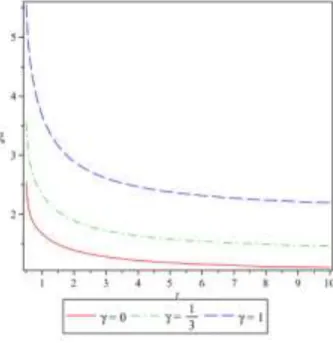
Figure 2: The plot of energy density  versus t for ₀ ₀ 0.1,₂ 1,₃ 0.5 .

4.1 Models with variable -term and constant 

Let us assume that the coefficient of bulk viscosity is constant, i.e. 

 

t  0  constant. Then the Eqs. (45)

and (46) together with (33) leads the following expressions for energy density, pressure and cosmological constant:









 

 

, 2

1 3

1

1 61 2 0

3 2 2

0 

  

 

          

      



 t

e t t

t t

(47)

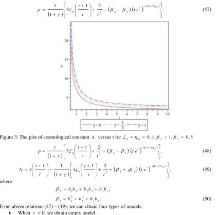
Figure 3: The plot of cosmological constant  versus t for ₀ ₀  0.1,₂ 1,₃  0.5









 

 

, 2

1 3

1

0

2 1 6 3

2 2

0 

  

 

          

      



 t

e t t

t t

p (48)









 

 

, 2

1 3

1 1 1

3 0

2 1 6 3

2 2

0 

  

 

          

        

      



t

e t t

t t t

t

(49)

where

1 3 3 2 2 1

2  bb  b b  b b

 ,

3 2 2 3 2 2

3  b  b  b b

 . (50)

From above relations (47) – (49), we can obtain four types of models:

ISSN: 2231-5373

http://www.ijmttjournal.org

Page 192

 When  =

3 1

, we obtain radiation dominated model.

 When  = –1, we have the degenerate vacuum or false vacuum or  vacuum model [42].

 When  = 1, the fluid distribution corresponds with the equation of state  = p which is known as Zeldovich fluid or stiff fluid model [43].

From Eq. (48), it is observed that the energy density  is a decreasing function of time and  > 0 always. The

energy density has been graphed versus time in Figure 2 for  = 0,

3 1

, 1. It is apparent that the energy density

remains positive in all three types of models. However, it decreases more sharply with the cosmic time in Zeldovich universe, compare to radiation dominated and empty fluid universes. Also it can be seen from the figure that  decreases more sharply with time in radiation dominated universe, compare to empty universe.

Figure 3 describes the variation of cosmological term  with time ( and  are in geometric units in entire

paper) for  = 0,

3 1

, 1. This is taken to be a representative case of physical viability of the models. In all three

types of models, we observe that  is decreasing function of time t and it approaches a small positive value at late time (i.e. at present epoch). However, it decreases more sharply with the cosmic time in empty universe, compare to radiation dominated and stiff fluid universes. The -term also decreases more sharply in radiation dominated universe, compare to stiff fluid universe.  positive cosmological constant resists the attractive gravity of matter due to its negative pressure and drives the accelerated expansion of the universe. Recent cosmological observations [30]-[32], [21] suggest the existence of a positive cosmological constant  with the magnitude 



Gh /c3



10 123 . These observations on magnitude and red-shift of type la supernova suggest that our universe may be an accelerating one with induced cosmological density through the cosmological  -term. Thus, the nature of  in our derived models are supported by recent observations.

4.2 Models with variable -term and   

Let us consider that   ₀ . In this case we obtain the expressions for energy density, pressure, bulk viscosity and cosmological constant as follows:



 

 

, 1

3

1 ₀

2 1 6 2

3 2 2 1 3 2 1

0

       

    

 

t t

e t b b b b b

b t

  



(51)



 

 

, 1

3

1 ₀

2 1 6 2

3 2 2 1 3 2 1

0

       



   

 

t t

e t b b b b b b p

t

 

 

ISSN: 2231-5373

http://www.ijmttjournal.org

Page 193

Figure 4: The plot of bulk viscosity coefficient  versus t for ₀ ₀  0.1,b₁  1, b₂  b₃  0.5



 

  , 1 3 1 ₀ 2 1 6 2 3 2 2 1 3 2 1 0 0                t t e t b b b b b b t      (53)

 

 



 

  , 1 3 1 1 3 0 2 1 6 2 3 2 2 1 3 2 1 2 1 6 2 2 0 0                            t t e t b b b b b b e t t

t _t t

     (54)

Figure 4 plots the variation of bulk viscosity coefficient  with time t. From this figure we observe that  is a positive decreasing function of time and it approaches to a constant quantity which is near to zero for all three

types of models  = 0,

3 1

, 1. This is in good agreement with physical behaviour of . However, it decreases

more sharply with the cosmic time in empty universe, compare to radiation dominated and Zeldovich universes.

4.3 Models with constant -term and variable 

 

t

In this case, the expressions for energy density, isotropic pressure and bulk viscosity coefficient are respectively, given by

 

  , 1 3 0 2 1 6 2 2                 t e t t t (55)

 

  , 1 3 0 2 1 6 2 2                  

   t   

e t t t p (56)





 

 











1



,

3 1 1 3 2 1 3 1 1 1 0 2 1 6 4 2                          t t t t e t t t t

t t 

 

  (57)

where

.

2 3

4  

  

From Eq. (55), it is observed that the energy density  is a decreasing function of time and  > 0 always.

Figure 5 : The plot of bulk viscosity coefficient  versus t for ₀  0.1,₄ 1   0

ISSN: 2231-5373

http://www.ijmttjournal.org

Page 194

types of models ,1.

3 1 , 0



 This is in good agreement with physical behaviour of . However, it decreases

more sharply with the cosmic time in empty universe, compare to radiating dominated and Zeldovich universes.

5. Discussion

In this paper, a class of cosmological models are presented with variable deceleration parameter q and cosmological term  in spatially homogeneous and anisotropic Bianchi type-I space-time in presence of bulk and shear viscosity. To find the explicit solution, we have considered a scale factor a

 

t  tet, which yields a time dependent deceleration parameter that affords a late time acceleration in the universe. The apprehension of the global evolution of the observationally amenable universe, mathematically encoded in the dynamics of its scale factor a, is of utmost importance in explaining practically all cosmological phenomena. One of the most intriguing aspects of this evolution is the recently established late-time transition from a decelerated to an accelerating regime of the expansion of the Universe. In this case, it is observed that as t  , q  1. This is the case of de Sitter universe. There is a Point Type singularity [41] at t = 0 in the model. The rate of expansion slows down and finally tends to zero as t 0. The spatial volume become infinitely large as t  , which would give essentially an empty universe.

References:

[1] L.M. Krauss and M.S. Turner, "The cosmological constant is Back", Gen. Rel. Grav. 27, 1137 (1995).

[2] S. Weinberg, "The cosmological constant problem", Rev. Mod. Phys. D. 61, 1 (1989)

[3] S.L. Adler, "Einstein gravity as a symmetry-breaking effect in quantum field theory", Rev. Mod. Phys. 54, 729 (1982).

[4] S. Weinberg, "A model of Leptons", Phys. Rev. Lett. 19, 1264 (1967).

[5] A.D. Linde, "Is the Lee constant a cosmological constant?", JETP Lett., 19, 183 (1974)

[6] J.M. Overduin and F.I. Cooper stock, "Evolution of the Scale factor with a variable cosmological Term", Phys. Rev. D 58, 043506 (1998).

[7] J.M. Overduin, "Non Singular Models with a variable cosmological Term.", Ap. J. 517, L. 1 (1999).

[8] J.M. Overdin, "Anisotropic Bianchi Type-I Magnetized String Cosmological Models with Decaying Vacuum Energy [1]

Density  (t).", Phys. Rev. D. 62, 102001 (2000).

[9] H. Liu and P.s. Wesson, "Universe Models with a variable "Cosmological" Constant and a 'big bounce'.", Asrophys. J. 562. 1 (2001).

[10] S. Podariu and B. Ratra, "Supernova Ia constraints on a Time-Variable cosmological 'Constant'.", Asrophys. J. 532, 109 (2000).

[11] K. Croswell, "Cosmological Consequences with Time dependent -term in Bianchi Type-I spa- _{time.", New Scientist, April 18}

(1994).

[12] P.J.E. Peebles and B. Ratra, "Cosmology with a time-variable cosmological 'constant'.", Astrophys. J. 325, L17 (1988).

[13] T. Banks, "Quantum gravity, the cosmological constant and all that", Nucl. Phys. B 249, 332 (1985).

[14] D.N. Spergel, et al., "Wilkinson Microwave Anisotropy Probe (WMPP)", Astrophys. J. Suppl. 170, 377 (2007);

astro-ph/0603449.

[15] D.J. Eisenstein, et al. "Deduction of the Baryon Acoustic Peak in the Large- Scale Correlation Function of SDSS Luminous Red

Galaxies", Astrophys. J. 633, 560 (2005).

[16] S.M. Carroll, "Why is the universe accelerating?", Conf. C0307282, TTH09, (2003) [AIP conf Proc 743, 16 (2005)].

[17] E.W. Kolb, S. Matarrese and A. Riotto, "On Cosmic Acceleration without dark energy", New J. Phys. 8 322 (2006).

[18] E.W. Kolb, S. Matarrese, A. Notari and A. Riotto, "Phantom field dynamics in loop quantum cosmology", arXiv:hep-th/0503117

(2005)

[19] A. Upadhey, M. Ishak and P.J. Steinhardt, "Dynamical dark energy : current constraints and forecasts", Phys. Rev. D 72, 063501

(2005).

[20] A.G. Riess, et al., "Type Ia Supernova Discoveries at z > 1 from the Hubble space Telescope : Post Deceleration and constraints

on Dark energy Evolution", Astrophys. J. 607, 665 (2004).

[21] A.G. Riess, et al., "Narrowing constraints on the early behaviour of dark energy", Astrophys J. 659, 98 (2007).

[22] R.A. Knop., et al., "High Red shift Supernovae observed with HST", Astrophys. J. 598, 102 (2003).

[23] S. Kalita, H.L. Dourah and K. Duorah, Indian J. Phys. 84, 629 (2010).

[24] S. Dey, J.P. Gewali, A.K. Jha, L. Chhaigle and Y.S. Jain, "Quantum dynamics of molecules in 4 He nano -droplets", Indian J.

Phys. 85, 1309 (2011).

[25] S. Oli, "Early Viscous Universe with Variable gravitational and cosmological 'constant'.", Indian J. Phys. 85, 755 (2012).

[26] Z. Nourinezhad and S.H. Mehdipour, "Gravitational energy of a non commutative Vaidya Black hole", Indian J. Phys. 86, 919

(2012).

[27] L.D. Landau and E.M. Lifshitz, "Fluid Mechanics, Pergamom", New York (1959) pp. 47.

[28] B. Saha, "Anisotropic cosmological models with a perfect fluid and a  term", Astsophye. Space Sci. 302. 83 (2006).

[29] B. Saha and V. Rikhvitsky, "Bianchi Type-I universe with viscous fluid and  term", Physica D 219, 169 (2006).

[30] S. Perl mutter, et al., "Discovery of a Supernova explosion at half the age of the universe", Nature 391, 51 (1998)

[31] S. Perl mutter, et al., "Measurement of omega and Lambda from 42 High-Redshift Supernovae", Astrophysical J. 517, 565 (1999).

[32] A.G. Riess, et al., "Observational Evidence from Supernovae for an Accelerating Universe and a cosmological constant", J. 116,

1009 (1998).

[33] S. Kumar and A.K. Yadav, "Some Bianchi Type-V Models of accelerating universe with dark energy", Mod. Phys. Lett. A 26,

647 (2011).

[34] A. Pradhan and H. Amirhashci, "Dark energy model in anisotropic Bianchi type-III space-time with variable EOS parameter",

ISSN: 2231-5373

http://www.ijmttjournal.org

Page 195

[35] H. Amirhashchi, A. Pradhan and H. Zainuddin, "An Interacting and Non-interacting Two-fluid dark energy models in FRW

universe with time dependent deceleration parameter", Int. J. Theo. Phys. 50, 3529 (2011).

[36] A. Pradhan, A.S. Dubey and R.K. Khare, "Some exact Bianchi type-I Cosmological Models in scalar-tensor theory of gravitation

with time dependent deceleration parameter", Rom. J. Phys. 57, 1222 (2012). [37] L. Amendola "Acceleration at Z > 1 ?", Mon. Not. R. Astron. Soc. 342, 221 (2003).

[38] A.G. Riess, et al., "Support for an accelerating universe and Glimpse of the epoch of deceleration", Astrophys. J. 560, 49 (2001).

[39] A. Pradhan and P. Pandey, "some Bianchi Type-I Viscose fluid Cosmological Models with a variable Cosmological constant",

Astrophys. Space Sce. 301, 127 (2006).

[40] C.P. Singh and S. Kumar, "Bianchi Type-I Viscous Fluid Cosmological Models with variable deceleration parameter", Astrophys

Space Sci. 323, 407 (2009).

[41] M.A.H. Mac Callum, "A Class of homogeneous cosmological models III : asymptotic behaviour", Common Math. Phys. 18,

2116 (1971).

[42] Y.M. Cho, "Reinterpretation of Jordan Barans- Dicke theory and Kaluza- Klein Cosmology", Phys. Rev. Lett. 68, 3133 (1992).

[43] Ya. B. Zeldovich, "The Equation of State of Ultrahigh Densities and its relativistic Limitations", Soviet Physics-JETP 14, 1143