https://doi.org/10.5194/bg-14-4295-2017 © Author(s) 2017. This work is distributed under the Creative Commons Attribution 3.0 License.
Bayesian calibration of terrestrial ecosystem models: a study of
advanced Markov chain Monte Carlo methods
Dan Lu1, Daniel Ricciuto2, Anthony Walker2, Cosmin Safta3, and William Munger4 1Computational Sciences and Engineering Division, Climate Change Science Institute, Oak Ridge National Laboratory, Oak Ridge, TN, USA
2Environmental Sciences Division, Climate Change Science Institute, Oak Ridge National Laboratory, Oak Ridge, TN, USA 3Sandia National Laboratories, Livermore, CA, USA
4School of Engineering and Applied Sciences, Harvard University, Cambridge, MA, USA
Correspondence to:Dan Lu ([email protected])
Received: 10 February 2017 – Discussion started: 22 February 2017
Revised: 30 June 2017 – Accepted: 30 August 2017 – Published: 27 September 2017
Abstract.Calibration of terrestrial ecosystem models is im-portant but challenging. Bayesian inference implemented by Markov chain Monte Carlo (MCMC) sampling provides a comprehensive framework to estimate model parameters and associated uncertainties using their posterior distributions. The effectiveness and efficiency of the method strongly de-pend on the MCMC algorithm used. In this work, a dif-ferential evolution adaptive Metropolis (DREAM) algorithm is used to estimate posterior distributions of 21 parameters for the data assimilation linked ecosystem carbon (DALEC) model using 14 years of daily net ecosystem exchange data collected at the Harvard Forest Environmental Measurement Site eddy-flux tower. The calibration of DREAM results in a better model fit and predictive performance compared to the popular adaptive Metropolis (AM) scheme. Moreover, DREAM indicates that two parameters controlling autumn phenology have multiple modes in their posterior distribu-tions while AM only identifies one mode. The application suggests that DREAM is very suitable to calibrate complex terrestrial ecosystem models, where the uncertain parameter size is usually large and existence of local optima is always a concern. In addition, this effort justifies the assumptions of the error model used in Bayesian calibration according to the residual analysis. The result indicates that a heteroscedastic, correlated, Gaussian error model is appropriate for the prob-lem, and the consequent constructed likelihood function can alleviate the underestimation of parameter uncertainty that is usually caused by using uncorrelated error models.
1 Introduction
Prediction of future climate heavily depends on accurate pre-dictions of the concentration of carbon dioxide (CO2) in the atmosphere. Predictions of atmospheric CO2 concentra-tions rely on terrestrial ecosystem models (TEMs) to simu-late the CO2exchange between the land surface and the at-mosphere. TEMs typically involve a large number of biogeo-physical and biogeochemical processes, the representation of which requires knowledge of many process parameters. Some parameters can be determined directly from experi-mental and measurement data, but many are also estimated through model calibration. Estimating these parameters in-directly from measurements (such as the net ecosystem ex-change (NEE) data) is a challenging inverse problem.
compared to other approaches in inverse problems, Bayesian inference not only estimates model parameters but also quan-tifies associated uncertainty using a full probabilistic descrip-tion.
Two types of Bayesian methods are widely used in param-eter estimation of TEMs, variational data assimilation (VAR) methods (Talagrand and Courtier, 1987) and Markov chain Monte Carlo (MCMC) sampling. VAR methods are compu-tationally efficient; however, they assume that the prior pa-rameter values and the observations follow a Gaussian distri-bution, and they require the model to be differentiable with respect to all parameters for optimization. In addition, VAR methods can only identify a local optimum and approximate the PPDF by a Gaussian function (Rayner et al., 2005; Ziehn et al., 2012). In contrast, MCMC sampling makes no as-sumptions about the structure of the prior and posterior dis-tributions of model parameters or observation uncertainties. Moreover, the MCMC methods, in principle, can converge to the true PPDF with an identification of all possible optima. Although it is more computationally intensive than VAR ap-proaches, MCMC sampling is being increasingly applied in the land surface modeling community (Dowd, 2007; Zobitz et al., 2011).
One widely used MCMC algorithm is adaptive Metropolis (AM) (Haario et al., 2001). For example, Fox et al. (2009) applied AM in their comparison of different algorithms for the inversion of a terrestrial ecosystem model; Järvinen et al. (2010) utilized AM for estimation of ECHAM5 climate model closure parameters; Hararuk et al. (2014) employed AM for improvement of a global land model against soil car-bon data; and Safta et al. (2015) used AM to estimate pa-rameters in the data assimilation linked ecosystem carbon model. The AM algorithm uses a single Markov chain that continuously adapts the covariance matrix of a Gaussian pro-posal distribution using the information of all previous sam-ples collected in the chain so far (Haario et al., 1999). As a single-chain method, AM has difficulty in traversing multidi-mensional parameter space efficiently when there are numer-ous significant local optima, and AM can be inefficient for estimating the PPDFs that exhibit strong correlations, as cor-related dimensions are better to be updated together (Vrugt, 2016). In addition, the AM algorithm uses a multivariate Gaussian distribution as the proposal to generate candidate samples and evolve the chain. AM, therefore, is particularly suitable for Gaussian-shaped PPDFs, but it may not converge properly to the distributions with multiple modes. Moreover, AM suffers from uncertainty about how to initialize the co-variance of the Gaussian proposal. Poor initialization of the proposal covariance matrix results in slow adaptation and in-efficient convergence.
The Gaussian proposal is also widely used in non-AM MCMC studies that involve TEMs. For example, Ziehn et al. (2012) used the Gaussian proposal for the MCMC simu-lation of the BETHY model (Knorr and Heimann, 2011) and Ricciuto et al. (2008, 2011) utilized the Gaussian proposal in
their MCMC schemes to estimate parameters in a terrestrial carbon cycle model. The single-chain and Gaussian-proposal MCMC approaches have limitations in sufficiently exploring the full parameter space and share slow convergence in sam-pling the non-Gaussian-shaped PPDFs and thus may end up with a local optimum with inaccurate uncertainty represen-tation of the parameters. Therefore, this poses a question on whether the AM and the widely used MCMC algorithms with Gaussian proposal generate a representing sample of the pos-terior distribution of the underlying model parameters. While we expect that computationally expensive sampling methods for parameter estimation yield a global optimum with an ac-curate probabilistic description, in reality we may in many cases obtain a local optimum with an inaccurate PPDF due to the limitations of these algorithms.
In this study, we employ the differential evolution adaptive Metropolis (DREAM) algorithm (Vrugt et al., 2008, 2009a; Lu et al., 2014) for an accurate Bayesian calibration of an ecosystem carbon model. The DREAM scheme runs multi-ple interacting chains simultaneously to explore the entire pa-rameter space globally. During the search, DREAM does not rely on a specific distribution, like the Gaussian distribution used in most MCMC schemes, to move the chains. Instead, it uses the differential evolution optimization method to gener-ate the candidgener-ate samples from the collection of chains (Price et al., 2005). This feature of DREAM eliminates the problem of initializing the proposal covariance matrix and enables ef-ficient handling of complex distributions with strong correla-tions. In addition, as a multi-chain method, DREAM can ef-ficiently sample multimodal posterior distributions with nu-merous local optima. Thus, the DREAM scheme is partic-ularly applicable to complex and multimodal optimization problems. Recently, Post et al. (2017) reported a successful application of DREAM in estimation of the complex Com-munity Land Model (CLM) using 1-year records of NEE ob-servations. They found that the posterior parameter estimates were superior to their default values in the ability to track and explain the measured NEE data.
(2) characterize parameter uncertainty in detail using accu-rately sampled posterior distributions; (3) investigate the ef-fects of model calibration methods on parameter estimation and model performance; and (4) justify the usage of the like-lihood function and explore the influence of the likelike-lihood function on the model calibration results. This work should provide ecological practitioners with valuable information on model calibration and understanding of the TEMs.
In the following Sect. 2, we first briefly summarize the general idea of Bayesian calibration and describe the AM and DREAM algorithms. Then in Sect. 3, we apply both al-gorithms to the DALEC model in a synthetic and a real-data study. Next in Sect. 4, we discuss the influence of the like-lihood function on parameter estimation and model perfor-mance. Finally in Sect. 5, we close this paper with our main conclusions.
2 Bayesian calibration and MCMC simulation 2.1 Bayesian calibration
Bayesian calibration of a model states that the posterior dis-tributionp(x|D)of the model parametersx, given observa-tion dataD, can be obtained from the prior distributionp(x)
ofx and the likelihood functionL(x|D)using Bayes’ theo-rem (Box and Tiao, 1992) via
p(x|D)=cL(x|D)p(x), (1)
wherecis a distribution represents the prior knowledge about the parameters. It is usually inferred from information of pre-vious studies at similar sites or from expert judgment. In the absence of prior information, a common practice is to use uninformative priors within relatively wide parameter ranges such that the prior distribution has little influence on the es-timation of the posterior distribution.
The likelihood function measures the model fits to the ob-servations. Selecting a likelihood function suitable to a spe-cific problem is still under study (Vrugt et al., 2009b). A commonly used likelihood function is based on the assump-tion that the differences between the model simulaassump-tions and observations are multivariate normally distributed, leading to a Gaussian likelihood such as the work of Fox et al. (2009), Hararuk et al. (2014), and Ricciuto et al. (2008, 2011). In this work, we also use the Gaussian likelihood, with het-eroscedastic and uncorrelated variances that are evaluated from the provided daily observation uncertainties. The as-sumptions of normality and independence are investigated by the residual analysis. In addition, we explore the influence of different choices of the likelihood function on the parameter estimation and model performance. The effect of data corre-lations on the inferred parameters was also assessed in our previous study (Safta et al., 2015).
2.2 MCMC sampling
In most environmental problems, the posterior distribution cannot be obtained with an analytical solution and is typi-cally approximated by sampling methods such as MCMC. The MCMC method approximates the posterior distribution by constructing a Markov chain whose stationary distribution is the target distribution of interest. As the chain evolves and approaches the stationary, all the samples after chain conver-gence are used for posterior distribution approximation, and the samples before convergence, which are affected by the starting states of the chain, are discarded.
The well-constructed MCMC schemes have been theoret-ically proven to converge to the appropriate target distri-bution p(x|D) under certain regularity conditions (Robert and Casella, 2004, p. 270). However, in practice the conver-gence rate is often impractically slow, which suggests that within a limited finite number of iterations, some inefficient schemes may result in an unrealistic distribution. The ineffi-ciency is typically resulted from an inappropriate choice of the proposal distribution used to generate the candidates. Ei-ther wide or narrow proposal distribution can cause ineffi-cient chain mixing and slow chain convergence (Geyer, 1992; Tierney, 1994). Hence, the definition of the proposal distribu-tion is crucial and determines the efficiency and the practical applicability of the MCMC simulation.
2.3 AM algorithm
The adaptive Metropolis (AM) algorithm is a modification to the standard Metropolis sampler (Haario et al., 2001). The key feature of the AM algorithm is that it uses a single Markov chain that continuously adapts to the target distribu-tion via its calculadistribu-tion of the proposal covariance using all previous samples in the chain. The proposal distribution em-ployed in the AM algorithm is a multivariate Gaussian dis-tribution with means at the current iterationxt and having a
covariance matrixCt that is updated along the chain
evolu-tion. To start the chain, AM first selects an arbitrary, strictly positive definite initial covarianceC0 according to the best prior knowledge that may be very poor. Then after a certain number of iterationsT, the covariance is updated based on the samples gained so far.
To apply the AM algorithm, an initial covarianceC0must be defined. The choice ofC0 critically determines the suc-cess of the algorithm. For example, in an extreme case, the variance of C0 is so large that no proposals are accepted within an iteration, and that the chain remains at the initial state without any movement. This situation continues as the chain evolves, and the use of updatedCt makes no
differ-ence because the variances ofCt are essentially zero since
prior knowledge about the target distribution. When such in-formation is not available, which is usually the case for com-plex models, some test simulations are needed. For exam-ple, Hararuk et al. (2014) inferred C0 from a test run of 50 000 simulations of a matrix approximation of the com-munity land model in estimating the PPDFs of soil carbon related parameters.
The construction ofCt is another critical influence on the
AM performance. In practice, some adjustments on Ct are
necessary to improve the AM efficiency. For example, when the chain does not have enough movement after a large num-ber of iterations, we can shrink Ct by some constant to
in-crease acceptance of new samples, and vice versa. The tech-niques used in the formulation of C0 and Ct improve the
AM efficiency in some degree for some problems. But, the computational cost spent on applying these techniques is not negligible (such as the test runs used for determining theC0) and some strategies require some artificial controls (such as manual adjustment of the scaling factor of Ct). Moreover,
determining a reasonable C0 and Ct becomes difficult for
high-dimensional problems.
To improve efficiency in high-dimensional case, Haario et al. (2005) extended the standard AM method to component-wise adaptation. This strategy applies AM on each parameter separately. The proposal distribution of each component is a 1-D normal distribution, which is adapted in a similar man-ner as in the standard AM algorithm, but the componentwise adaptation does not work very well for distributions with a strong correlation. Safta et al. (2015) applied an iterative al-gorithm to break the original high-dimensional problem into a sequence of steps of increasing dimensionality, with each intermediate step starting with an appropriate proposal co-variance based on a test run. This technique provided a rather reasonable proposal distribution, but the computational cost used to define the proposal was rather high.
AM is a single-chain method. As a single chain, it may suf-fer from some difficulties in judging the convergence. Some-time the most powerful diagnostics cannot guarantee that the chain has converged to the target distribution (Gelman and Shirley, 2011). One solution to alleviate the problem is running multiple independent chains with widely dispersive starting points and then using the diagnostics for multi-chain schemes, such as the univariateRˆ statistic (Gelman and Ru-bin, 1992) and the multivariateRˆ statistic (Brooks and Gel-man, 1998), to check convergence. When the chain has a good mixing and all the chains converge to the same PPDF, theRˆ value is close to one, and in practice the threshold of 1.2 is usually used for convergence diagnosis. On the other hand, when the chain does not mix well and different chains converge to the different portion of the target distribution, it is unlikely that theRˆ will reach the value of 1.2 required to declare convergence. Generally, this situation suggests that multiple modes exist in the target PPDF and the MCMC al-gorithm is unable to identify all the modes.
2.4 DREAM algorithm
The DREAM algorithm is a multi-chain method (Vrugt, 2016). Multi-chain approaches use multiple chains running in parallel for global exploration of the posterior distribution, so they have several desirable advantages over the single-chain methods, particularly when addressing complex prob-lems involving multimodality and having a large number of parameters with strong correlations. In addition, the applica-tion of multiple chains allows utilizing a large variety of sta-tistical measures to diagnose the convergence including the
ˆ
Rstatistics mentioned above.
DREAM uses the Differential Evolution Markov Chain (DE-MC) algorithm (ter Braak, 2006) as its main building block. The key feature of the DE-MC scheme is that it does not specify a particular distribution as the proposal but pro-poses the candidate points using the differential evolution method based on current samples collected in the multiple chains. Thus, DE-MC can apply to a wide range of problems whose distribution shapes are not necessarily similar to the proposal distribution, and it also removes the requirement of initializing the covariance matrix as in AM. In addition, the DE-MC can successfully simulate the multimodal distribu-tions, because it directly uses the current location of the mul-tiple chains to generate candidate points, allowing the possi-bility of direct jumps between different modes.
The DREAM algorithm maintains the nice features of the DE-MC but greatly accelerates the chain convergence. More information about the DREAM algorithm was presented in Vrugt et al. (2008, 2009a), Laloy and Vrugt (2012), Lu et al. (2014), and Vrugt (2016).
2.5 Strategies and capabilities of AM and DREAM in sampling complex problems
Since multimodality is a potential feature of complex prob-lems including terrestrial ecosystem models (Stead et al., 2005; Thibault et al., 2011), it is important to understand the strategies of AM and DREAM and to investigate their capa-bilities in sampling the multimodal distributions.
the beginning by using a large covariance matrix of the pro-posal, and then the proposal covariance is reduced by a freely chosen scale factor if the parameters do not have significant movement. By creating multiple proposal stages, DRAM en-ables an extensive search and meanwhile alleviates the over-shooting problem and improves the acceptance rate. How-ever, as dimensionality increases, the multimodality becomes more difficult for the algorithms using the Gaussian proposal because it is highly likely different dimensions have differ-ent variances and a constant scaling factor can only shrink the covariance simultaneously.
In contrast, DREAM is designed for sampling high-dimensional and multimodal problems by running multiple different chains simultaneously for global exploration. It au-tomatically tunes the scale and orientation of the proposal in randomized subspaces during the search (Vrugt et al., 2009a). As DREAM directly uses the current location of the multiple chains, instead of the covariance of the Gaus-sian proposal, to generate candidate points, it enables di-rect jumps between different modes (including the relatively far disconnected modes) as long as the initial samples of the chains are widely distributed over the parameter space. Laloy and Vrugt (2012) demonstrated that DREAM can suc-cessfully sample a 25-dimensional trimodal distribution with equal separation of 10 units between modes. However, for the same problem with the same number of function evalu-ations, AM and DRAM converged to only one mode. Note that to sample a distribution with many modes, one needs to have some prior information about their rough locations; oth-erwise no methods can guarantee finding all the modes, es-pecially when the distance between the modes is very large and not a constant.
3 Application to a terrestrial ecosystem model
In this section, we applied the DREAM algorithm to the data assimilation linked ecosystem carbon (DALEC) model to es-timate the posterior distributions of its parameters. In com-parison, the AM algorithm was also applied. DALEC is a rel-atively simple carbon pool and flux model designed specif-ically to enable parameter estimation in terrestrial ecosys-tems. We used DALEC to evaluate the performance of AM and DREAM in model calibration; we compared their ac-curate simulations of the parameter PPDFs, model’s good-ness of fit, and predictive performance of the calibrated mod-els. Previous studies based on MCMC methods that used Gaussian proposals have not reported multimodality in the marginal PPDFs of the model parameters, so it is important to know whether the parameters have multimodality; if the multimodality exists, we assess whether or not DREAM can identify the multiple modes and improve the calibration re-sults and thus the predictive performance.
3.1 Description of the model and parameters for optimization
The DALEC v1 model is used here (Williams et al., 2005; Fox et al., 2009) with some structural modifications (Safta et al., 2015). DALEC consists of six process-based submodels that simulate carbon fluxes between five major carbon pools: three vegetation carbon pools for leaf, stem, and root and two soil carbon pools for soil organic matter and litter. The fluxes calculated on any given day impact carbon pools and pro-cesses in subsequent days.
The six submodels in DALEC are photosynthesis, phenol-ogy, autotrophic respiration, allocation, litterfall and decom-position. Photosynthesis is driven by the aggregate canopy model (ACM) (Williams et al., 2005), which itself is cali-brated against the soil–plant–atmosphere model (Williams et al., 1996). DALEC v1 was modified to incorporate the phe-nology submodel used in Ricciuto et al. (2011), driven by six parameters. This phenology submodel controls the cur-rent leaf area index (LAI) proportion of the seasonal maxi-mum LAI (laimax). Spring LAI growth is driven by a linear relationship to growing degree days (gdd), while senescence and LAI loss are driven by mean air temperature. To sim-plify our model structure, senescence and LAI loss are con-sidered to occur simultaneously. In reality, leaves may still be present on the trees but photosynthetically inactive due to the loss of chlorophyll. Here, this inactive LAI is considered to have fallen and is added to the litter pool. To further reduce model complexity, the plant labile pool in DALEC v1 was removed and a small portion of stem carbon is instead re-moved to support springtime leaf growth each year. The six phenology parameters are a threshold for leaf out (gdd_min), a threshold for maximum leaf area index (gdd_max), the tem-perature for leaf fall (tsmin), seasonal maximum leaf area in-dex (laimax), the rate of leaf fall (leaffall), and leaf mass per unit area (lma), respectively. Given the importance of main-tenance respiration in other sensitivity analyses (Sargsyan et al., 2014), we expanded the autotrophic respiration submodel to explicitly represent growth respiration (as a fraction of car-bon allocated to growth) and maintenance respiration with the base rate and temperature sensitivity parameters.
So for the first three plant submodels, deciduous phenol-ogy has six parameters; ACM shares one parameter, lma, with the deciduous phenology and employs two additional parameters, leaf C : N ratio (which is fixed at a constant of 25 in the simulation) and photosynthetic nitrogen use efficiency (nue); and the autotrophic respiration model computes the growth and maintenance respiration components and is con-trolled by three parameters, the growth respiration fraction (rg_ frac), the base rate at 25◦C (br_mr), and temperature sensitivity for maintenance respiration (q10_mr).
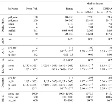
Table 1.Nominal values and ranges of the 21 parameters for optimization in the DALEC model, and the maximum a posteriori (MAP) estimates based on the AM and DREAM samplers.
MAP estimates
ParName Nom. Val. Range AM DREAM
LL= −6662.6 LL= −6578.3
Decid.
Phen.
gdd_min 100 10–250 37.90 39.53
gdd_max 200 50–500 203.44 201.77
tsmin 5 0–10 4.88 7.87
laimax 4 2–7 2.01 2.00
leaffall 0.1 0.03–0.95 0.067 0.035
lma 80 20–150 136.81 147.45
A
CM nue 7 1–20 8.90 8.21
A.
R. q10_mr 2 1–4 1.00 1.00
br_mr 10−4 10−5–10−2 7.39×10⁻³ 6.35×10⁻³
rg_frac 0.2 0.05–0.5 0.06 0.066
A. astem 0.7 0.1–0.95 0.75 0.74
Lit.
F
al. tstem 1/(50×365) 1/(250×365)–1/(10×365) 1.98×10⁻⁵ 1.63×10⁻⁵ troot 1/(5×365) 1/(25×365)–1/365 8.55×10⁻⁴ 7.88×10⁻⁴
Decomp.
q10_hr 2 1–4 2.98 2.68
br_lit 1/(2×365) 1/(5×365)–10/(5×365) 4.97×10⁻³ 5.36×10⁻³ br_som 1/(30×365) 1/(100×365)–1/(10×365) 2.79×10⁻⁵ 2.88×10⁻⁵
dr 10−3 10−4–10−2 2.46×10⁻³ 3.39×10⁻³
Init.
C.
stemc_init 5000 1000–15 000 1070.9 1417.8
rootc_init 500 100–3000 100.56 100.61
litc_init 600 50–1000 60.74 66.77
somc_init 7000 1000–25 000 2029.1 4708.2
Parameter units refer to Table 1 of Safta et al. (2015). The LL represents the log likelihood evaluated at the MAP parameter estimates; the larger the value is, the better the model fit.
stem allocation parameter (astem). The litter fall model re-distributes the carbon content from vegetation pools to lit-ter pools and is based on the turnover times for stem (tstem) and root (troot). The last submodel is a decomposition model that simulates heterotrophic respiration and the decomposi-tion of litter into soil organic matter (SOM). This model is driven by the temperature sensitivity of heterotrophic respi-ration (q10_hr), the base turnover times for litter (br_lit) and SOM (br_som) at 25◦C, and by the decomposition rate (dr) from litter to SOM.
Model parameters are summarized in Table 1. These pa-rameters were grouped according to the six submodels that employ them, except for lma, which impacts both the de-ciduous leaf phenology and ACM. The nominal values and numerical ranges for these parameters were designed to re-flect average values and broad uncertainties associated with the temperate deciduous forest plant functional type that in-cludes Harvard Forest (Fox et al., 2009; White et al., 2000; Ricciuto et al., 2011). Observed air temperature, solar
radia-tion, vapor pressure deficit, and CO2concentration were used as boundary conditions for the model.
In order to reduce computational time, we employed tran-sient assumptions for running DALEC. That is, for any given set of parameter values, DALEC was run one cycle only for 15 years between 1992 and 2006 where observation data are available. Under this assumption, four additional parameters were used to describe the initial states of two vegetation car-bon pools (stemc_init androotc_init) and the two soil car-bon pools (litc_initandsomc_init), as also summarized in Table 1. Thus, a total of 21 parameters were considered and estimated in this study. To avoid the influence of prior dis-tributions on the investigation of the posteriors estimated by AM and DREAM, uniform priors were used for all parame-ters with the ranges specified in Table 1.
3.2 Calibration data
95 100 105 0 0.5 1 gdd_min Marginal PPDF
190 200 210 0
0.1 0.2 0.3
gdd_max 3 4 5
0 0.5 1 1.5
laimax 4.5 5
0 5 10
tsmin
DREAM AM True value
0.09 0.1 0.11 0
100 200 300 400
leaffall 4 6 8
0 0.5 1
nue 0.15 0.2 0.25 0 10 20 30 rg_frac 5 10
x 10−4 0
1 2
x 104
br_mr
Marginal PPDF
1 2 3 4
0 0.2 0.4 0.6 0.8
q10_mr 0.2 0.4 0.6 0.8 0
1 2 3
astem 0.5 1 1.5 2 2.5x 10⁻³
0 500 1000 1500
troot 0.5 1 1.5 2 2.5x 10⁻⁴
0 5000 10000
tstem 1.8 2 2.2
0 5 10 15 20
q10_hr 1 1.5 2x 102.5−3
0 500 1000 1500 2000 br_lit
0.5 1 1.5 2 2.5 x 10⁻⁴ 0
1 2
x 104
br_som
Marginal PPDF
2 4 6 8 x 10⁻³ 0
200 400
dr 50 100
0 0.02 0.04 0.06
lma 5000 10000 15000 0
0.5 1 1.5
x 10−4
stemc_init 1000 2000 3000 0
0.5 1
x 10−3
rootc_init 500 1000
0 1 2
x 10−3
litc_init 0.5 1 1.5 2x 102.54
0 0.5 1
x 10−4
[image:7.612.53.545.70.273.2]somc_init
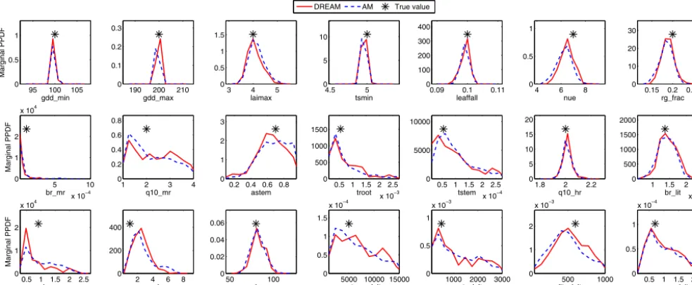
Figure 1.Estimated marginal posterior probability density functions (PPDFs) of the 21 parameters using the AM and DREAM algorithms, along with the true parameter values to generate the pseudo-data in the synthetic case.
the NACP site synthesis study (Barr et al., 2013) based on flux data measured at the site (Urbanski et al., 2007). The daily observations cover a period of 15 years starting with the year 1992 and part of the data in the year 2005 is miss-ing. Hill et al. (2012) estimated that daily NEE values fol-lowed a normal distribution, with standard deviations esti-mated by bootstrapping half-hourly NEE data (Papale et al., 2006; Barr et al., 2009). These standard deviations have val-ues between 0.2 and 2.5, with the mean value about 0.7. To-tal 14 years 5114 NEE data (years from 1992 to 2004 and year 2006) were considered here for model calibration and their corresponding standard deviations were used to con-struct the heteroscedastic, diagonal covariance matrix of the Gaussian likelihood function by assuming the data were un-correlated. In Sect. 4, we examine the independent, Gaussian error assumption using residual analysis and investigate the influence of error models on parameter estimation and model performance.
3.3 Synthetic study with pseudo-data
We first applied AM and DREAM to a synthetic case to eval-uate their capability in parameter estimation. The same peri-ods of daily NEE data were generated with the nominal pa-rameter values in Table 1. These synthetic data for calibra-tion were then corrupted with Gaussian errors having means at zero and the same standard deviations with the observed NEEs.
DREAM launched 10 parallel chains starting at values randomly drawn from the parameter prior distributions. AM used one chain and the chain has the same initialization with DREAM. In addition, AM also requires the initialization of the covariance matrix of its Gaussian proposal. We first drew
some samples from the parameter space and computed the initial covariance. However, this initialization caused a slow convergence of AM with an extremely small acceptance rate (about 0.01 % after 1×10⁵iterations). The reason could be that for this rather high-dimensional problem with very di-verse parameter ranges, the candidate samples are easily out-side the target distribution when they are drawn from the Gaussian proposal. To facilitate the AM convergence, we started the chain from the true parameter values and con-structed the initial covariance from samples around the true values. This setup can only be done in a synthetic case with information of true parameters available; practically it needs some test runs to get information about the underlying distri-butions. In addition, this initialization of AM makes an un-fair comparison with DREAM that launched chains blindly, but on the other hand, it suggests DREAM’s ease of use and setup, its robustness and efficiency.
Chain convergence was assessed via the Gelman–Rubin
ˆ
Rstatistics. Figure 1 presents the estimated marginal PPDFs of the 21 parameters from both AM and DREAM samples after convergence along with their true values. The two al-gorithms produce very similar distributions that both enclose the true values very well. All the parameters show one mode in their PPDFs and the true values are located or close to the modes. The results indicate that for this unimodal prob-lem both algorithms can successfully infer the underlying parameter distributions, although AM needs a proper initial-ization for its convergence. To further evaluate the calibra-tion accuracy, we investigate the sum of squared weighted residuals (SSWR) for the optimal parameters. If the param-eter optimization is reasonable, the calculated SSWR should follow a chi-squared distribution with its mean equal to the
minus the number of calibrated parameters, in this study
k=5114−21=5093. The resulted SSWR is 5044 close to the mean value 5093 of the chi-squared distribution. This once again suggests the accuracy and reasonability of our pa-rameter estimation.
In addition, Fig. 1 indicates that about half of the parame-ters are well constrained, when we define a well-constrained parameter as its posterior distribution occupying at most half the range of the prior distribution (Keenan et al., 2013). This result is consistent with some of previous studies on DALEC calibration using NEE data alone. For example, in the syn-thetic study of Fox et al. (2009), their MCMC simulation (M1) showed that 16 of 17 parameters were well constrained. Similarly, the synthetic study in Hill et al. (2012) indicated that 20 of 23 parameters had their 90 % confidence intervals occupy less than half of the prior range.
Whether a parameter is identifiable depends on the model, model parameters, and the calibration data. When the param-eter related processes are necessary to simulate the model outputs whose corresponding observation data are sensitive to the parameters, the parameters can usually be identified and sometimes well constrained. For example, Keenan et al. (2013) showed that in their FöBAAR model with 40 pa-rameters, many parameters could not be constrained even with the consideration of several data streams together. They found that these unidentifiable parameters might be redun-dant in the model structure representation. Roughly speak-ing, for a simple model with a few number of parameters, the parameters can be more identifiable than the complex models with a large parameter size (Richardson et al., 2010; Weng and Luo, 2011). On the other hand, if the calibration data are sensitive to the parameters, even a complex model can some-times be well constrained by using a single type of observa-tions. For example, Post et al. (2017) estimated eight CLM parameters using 1-year records of half-hourly NEE observa-tions at four sites, and found that for most sites the CLM pa-rameters can be well constrained with their 95 % confidence intervals close to the maximum a posteriori estimates. For the only site where the parameter uncertainties were relatively large, they concluded that the simulated NEE was less sen-sitive to these parameters. In our and those synthetic studies of Fox et al. (2009) and Hill et al. (2012), all the parameter related processes are necessary for DALEC simulation and most parameters were shown to be sensitive to the observa-tion data (Safta et al., 2015), this explains to some extent that many DALEC parameters can be well constrained in these synthetic studies.
3.4 Real-data study
In the real-data study, the measured NEE data with given standard deviations were used for DALEC calibration. Both AM and DREAM algorithms were applied to infer the un-known parameters. Different from the synthetic case, the real-data study involves model structural errors besides the
2e61 2.2e6 2.4e6 2.6e6 2.8e6 3e6 1.2
1.4 1.6 1.8 2
(a) AM
Univariate Multivariate
2e51 2.2e5 2.4e5 2.6e5 2.8e5 3e5 1.2
1.4 1.6 1.8 2
Iteration
[image:8.612.311.546.66.344.2](b) DREAM
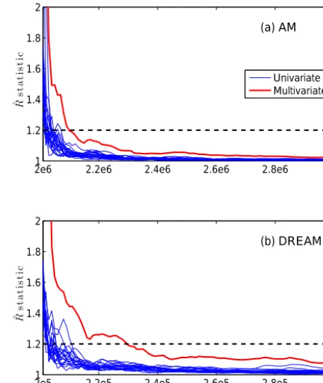
Figure 2.Univariate and multivariate Gelman–RubinRˆ statistics
(a)for the last 1 000 000 iterations from 10 independent AM runs and(b)for the last 100 000 iterations from the DREAM simulation using 10 interacting chains. The values less than the threshold of 1.2 suggest chain convergence.
measurement errors. We again use the heteroscedastic, un-correlated, Gaussian likelihood function for calibration and examine these error assumptions in Sect. 4 through residual analysis.
DREAM launched 10 parallel chains starting at values ran-domly drawn from the parameter prior distributions, and each chain evolved 300 000 iterations. Chain convergence was assessed via both the univariate and multivariate Gelman– RubinRˆstatistics. Figure 2b plots theRˆvalues of the 21 pa-rameters for the last 100 000 iterations. The figure suggests that the last 50 000 samples of each chain (i.e., total 500 000 samples from 10 chains) can be used for the PPDF approxi-mation as theRˆhas values below the threshold of 1.2.
AM used one chain and the chain has the same initializa-tion of the first sample with DREAM. For the initializainitializa-tion of the Gaussian covariance in the AM proposal, we first drew some samples from the parameter space and constructed the covariance. However, this initialization caused a high rejec-tion rate and ended up with essentially a single parameter state after hundreds of thousands of iterations. To facilitate the convergence of AM, we constructed the initial covariance based on the first 200 000 samples from the DREAM simula-tion. We conducted 10 independent AM runs, so the sameRˆ
30 40 50 0 0.1 0.2 0.3 gdd_min Marginal PPDF
180 200 220
0 0.05 0.1 0.15
gdd_max 2 2.05 2.1
0 50 100 laimax DREAM AM
4 6 8
0 5 10 15 20
tsmin 0.02 0.04 0.06 0.08
0 200 400 600
leaffall 6 8 10 12
0 0.5 1 1.5
nue 0.06 0.08 0.1
0 50 100
rg_frac
6 8 10
x 10−3
0 500 1000 1500 br_mr Marginal PPDF
1 1.02 1.04
0 50 100 150
q10_mr 0.6 0.7 0.8 0.9
0 10 20 30
astem 0.5 1 1.5x 10⁻³
0 2000 4000 6000
troot 2 4 x 10−56
0 0.5 1 1.5 2
x 105
tstem 2 3 4
0 1 2 3
q10_hr 3.5 4 4.5 x 10⁵ −3
0 2000 4000 6000
br_lit
3 3.5 4
x 10−5
0 2 4
6x 10
5
br_som
Marginal PPDF
2 4 6
x 10−3
0 500 1000
dr 100 120 140
0 0.05 0.1
lma 3000 7000
0 2 4 6
8x 10
−4
stemc_init 100 105 110 115
0 0.1 0.2 0.3 0.4
rootc_init 100 200 300 400 500
0 0.005 0.01 0.015
litc_init 3000 7000 11000
0 2 4
6x 10
−4
[image:9.612.55.546.64.256.2]somc_init
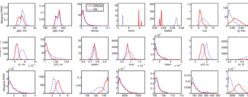
Figure 3.Estimated marginal posterior probability density functions (PPDFs) of the 21 parameters using the AM and DREAM algorithms in the real-data study.
chain simulated 3 000 000 samples, so that the number of function evaluations in one AM chain is the same as that of DREAM using 10 chains. The Rˆ values of all parameters based on the 10 AM runs for the last 1 000 000 iterations are shown in Fig. 2a. The figure indicates that AM has converged and the last 500 000 samples from one chain were used for the PPDF approximation.
The estimated PPDFs from AM and DREAM are pre-sented in Fig. 3, and the optimal parameter estimates, as rep-resented by the maximum a posteriori (MAP), are summa-rized in Table 1. Figure 2 shows that more than half of the parameters are constrained and some well-constrained pa-rameters are edge hitting, where the mode of these param-eters occur near one of the edges of their allowable ranges and most of the parameter values are clustered near the edge such asstemc_init,rootc_init, andlitc_init. As we can see in the synthetic case, these edge-hitting parameters (e.g.,tstem,
stemc_init,rootc_init, andlitc_init) have wide confidence tervals that almost occupy the entire allowable ranges, in-dicating that the NEE data should provide little informa-tion about these parameters. This edge-hitting behavior may be caused by a compensation for model structural errors and data biases (Braswell et al., 2005), and we do not con-sider these edge-hitting parameters to be well constrained despite small posterior uncertainties. The tight uncertainty bounds on these parameters are likely unrealistic and could contribute to overconfidence in model predictions. However, quantifying model structural error is an on-going research topic and no formal results have been published to our knowl-edge. We will investigate the influence of model structural errors on parameter estimation in future studies.
In comparison of the results between AM and DREAM, Fig. 3 indicates that they produce very similar PPDFs for many parameters, such as gdd_max, laimax, br_som,
stemc_init, and rootc_init; however, for parameters tsmin
andleaffall, their estimated PPDFs are substantially differ-ent. This also can be seen in Table 1 where the differences of MAP values for most parameters are relatively small be-tween the two algorithms, the relative difference for tsmin
andleaffallis 38 and 94 %, respectively. The parametertsmin
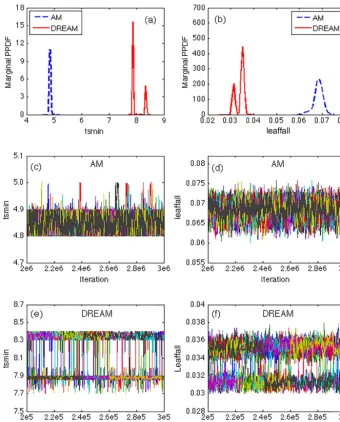
represents the temperature triggering leaf fall and the leaf-fall represents the rate of leaf fall on days when the tem-perature is belowtsmin. We further analyze the simulations of these two parameters from AM and DREAM in Fig. 4. Figure 4a and b illustrate two separated modes in the esti-mated marginal PPDFs oftsminandleaffallobtained from DREAM, while AM only identifies one mode for both pa-rameters and they dramatically differ from any modes sim-ulated by DREAM. For example, the single mode oftsmin
identified by AM gives a lower temperature threshold (mean-ing a later initiation of senescence) that is compensated for by a higher estimate ofleaffallrate compared to DREAM. As shown in the trace plots of Fig. 4c and d, all 10 indepen-dent runs of AM converged to a single mode, with values
of tsminbetween 4.8 to 5.0 and values of leaffallbetween
0.06 and 0.075. In contrast, each of the 10 parallel chains of DREAM, as exhibited in Fig. 4e and f, jumps back and forth between two modes. And the two parameters compensate for each other by jumping in opposite directions, wheretsminis more likely to be near the mode with a smaller value of 7.9 than that of 8.35 andleaffallis more likely to be near the mode of a larger value of 0.035 than that of 0.031.
Figure 4.AM and DREAM results for parameterstsminandleaffallin the DALEC model. The estimated marginal posterior distributions of
(a)tsminand(b)leaffall; Trace plots of(c)sampledtsminand(d)sampledleaffallwith AM using 10 independent chains; and trace plots of
(e)sampledtsminand(f)sampledleaffallwith DREAM using 10 interacting chains. The evolution of each chain is coded with a different color.
with the correlation coefficient of −0.95. As demonstrated in Fig. 5b, the samples oftsminandleaffallfrom DREAM fall almost perfectly on the line with slope of−1, where the mode with smallertsminvalues corresponds to the mode of largerleaffalland the similar correspondence can be found for the other pair of modes.
The existence of two modes fortsminandleaffalland the negative correlation between the two parameters are not un-reasonable as we used multiple years of observations for pa-rameter estimation. It is possible that in some years the senes-cence is triggered later (i.e., a smallertsmin) but proceeds at a faster rate (i.e., a largerleaffall), while in some other years the senescence is triggered earlier (i.e., a larger tsmin) but
proceeds at a slower rate (i.e., a smallerleaffall). Given our model simplification of concurrent senescence and leaf fall and our use of NEE rather than LAI observations as a con-straining variable, we note that these optimized parameters are more likely to reflect the process of chlorophyll loss than actual leaf loss. Cool temperatures are a key driver of senes-cence at this site (Richardson et al., 2006).
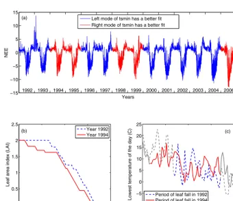
Figure 6a highlights the years in red where the model based on the right mode oftsminand the left mode of senes-cence rate (leaffall) has a better fit to the observed NEE, i.e., years 1994, 1995, 1998, 1999, and 2006. The remaining years are highlighted in blue where the left mode oftsmin
Figure 5.Posterior distributions of parameterstsminandleaffallsimulated by(a)AM and(b)DREAM. AM simulation results exhibit a negligible correlation coefficient (corr) between the two parameters with a value of−0.042, while DREAM results show that the two parameters are strongly correlated with the corr value of−0.95.
−15 −10 −5 0 5 10 15
1992 1993 1994 1995 1996 1997 1998 1999 2000 2001 2002 2003 2004 2006 Years
NEE
(a) Left mode of tsmin has a better fit Right mode of tsmin has a better fit
Sep. 10 Sep. 20 Oct. 10 Oct. 30 Nov. 20 0.5
1 1.5 2 2.5
Leaf area index (LAI)
(b) Year 1992
Year 1994
Sep. 1 Sep. 20 Oct. 10 Oct. 30 Nov. 20 −10
−5 0 5 10 15 20 25
Lowest temperature of the day (C)
(c)
Period of leaf fall in 1992 Period of leaf fall in 1994
Figure 6. (a)Observed NEE with years highlighted in red where the left mode oftsminhas a better model fit and years highlighted in blue where the right mode oftsminhas a better model fit;(b)the simulated leaf area index (LAI) of years 1992 and 1994; and(c)the recorded lowest temperature of years 1992 (blue) and 1994 (red). The blue and red lines in(c)highlight the corresponding periods of leaf fall until LAI becomes zero for 1992 and 1994, respectively. The color scheme is synchronized between(a),(b), and(c)frames. Note that decreases in LAI as predicted by our simplified version of DALEC reflect chlorophyll loss rather than leaf drop.
Taking years 1992 and 1994 as an example, we examined the leaf area index (LAI) in the period of senescence. Fig-ure 6b shows that at the first few days of September in both years, the values of LAI were the same around 2.0; after that the timing of senescence during the two years differs
[image:11.612.126.467.282.576.2]LAI remained near the maximum value during all of Septem-ber, then dropped rapidly in October and hit zero also on 7 November; this process took about 40 days. The changes in the LAI between the two years reflect the variability in the time of year when the leaves start to drop and the rate of leaf drop. Although the leaf fall in 1992 was triggered later than in 1994, the leaves in 1992 dropped at a faster rate, resulting in LAI approaching zero at the same time of the year.
Figure 6c depicts the recorded lowest temperature of the days between 1 September and 20 November for years 1992 and 1994, where the red line highlights the period between the first leaf and the last leaf drops in 1994. The blue line highlights the corresponding period of leaf fall in 1992. Since the senescence was triggered in the early September of 1994, the temperature of triggering leaf fall was relatively high, about 8.1◦C (associated with the higher mode oftsmin) as shown in Fig. 6c. In the rest days of September in 1994 fol-lowing the senescence trigger, temperatures remained warm. The slower leaf fall rate associated with periodic warm con-ditions (temperatures above tsmin) and the lower mode of
leaffallcaused a slow leaf fall in September of 1994 as shown in Fig. 6b. In comparison, in 1992, senescence was triggered at the end of September with a low temperature of 2.6◦C. Then in October with colder temperatures, the leaves drop at a rapid rate associated with the consistent cold temperatures and higher mode of leaffall. Especially in late October, the temperatures are consistently belowtsmin, causing a fast rate of leaf fall, as shown in Fig. 6b, where the decreasing rate of the LAI in the late October of 1992 is very large. This indi-cates that a higher temperature trigger is usually associated with a lower leaf fall rate and vice versa.
The bimodality identified in the DREAM simulation and examined in the scenarios above reflects the inability of the model structure to predict the observations consistently with a single set of parameters. This bimodality examined in DREAM may be caused in part by an incomplete representa-tion of the senescence process. Using a temperature threshold (parametertsmin) and a constant rate of leaf fall (parameter
leaffall) to predict senescence is almost certainly an oversim-plification. In reality, the process of senescence is also af-fected by day length. Longer days and warmer temperatures cause a relatively slow rate of leaf fall, whereas shorter days and cooler temperatures accelerate the rate that the leaves fall (Leigh et al., 2002; Saxena, 2010). The higher mode oftsmin
means that senescence is initiated earlier, when day lengths are still relatively long. This may partially explain why this mode is associated with a lower mode of theleaffall param-eter. Other factors not represented in DALEC are also likely to play a role such as soil moisture, or a more complex rela-tionship with spring phenology (Keenan et al., 2014, 2015).
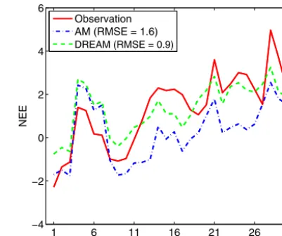
The difference in estimated parameters between AM and DREAM causes different simulations of NEE, especially during the autumn. As an example, Fig. 7 illustrates the com-parison of the simulated NEE to observations for a month in autumn of the year 1995 based on MAP estimates obtained
1 6 11 16 21 26 31
−4 −2 0 2 4 6
October 1995
NEE
Observation AM (RMSE = 1.6)
[image:12.612.325.526.66.234.2]DREAM (RMSE = 0.9)
Figure 7.Simulated NEE values based on the optimal parameters (i.e., the MAP values listed in Table 1) estimated by the AM and DREAM algorithms in October 1995. The root mean square error (RMSE) indicates that DREAM produces a better model fit than AM.
under AM and DREAM. Visual inspection indicates that the simulated NEE from the DREAM-calibrated parameters pro-vides a better fit to the observations, as also indicated by the smaller root mean squared errors (RMSEs). In addition, the maximum log likelihoods listed in Table 1 suggest that over-all the DREAM-estimated parameters produce a better model fit to the observations, comparing−6578.3 with the smaller AM value of−6662.6.
3.5 Assessment of predictive performance
To further compare the calibration results between AM and DREAM, we explore their predictive skills based on the sam-pled PPDFs of model parameters. We employed the Bayesian posterior predictive distribution (Lynch and Western, 2004) to assess the adequacy of the calibrated models. Specifi-cally, the posterior distribution for the predicted NEE data,
p(y|D), is represented by marginalization of the likelihood over the posterior distribution of model parametersxas
p(y|D)=
Z
p(y|x)p(x|D)dx. (2)
In approximation ofp(y|D), we used the converged MCMC samples fromp(x|D). The last 500 samples of each chain (total 500×10=5000 samples) were considered; for each parameter sample we drew 20 samples of the 14 years NEE data from their normal distributions, where the mean values are the model simulations. Then the total 100 000 prediction samples were used to approximate the posterior predictive densityp(y|D).
−10 −5 0 5 10
NEE
AM
J F M A M J J A S O N D Predictive coverage is 73.4 %; CRPS = 0.48
95 % confidence interval Observation
−10 −5 0 5 10
Year 1995
NEE
DREAM
[image:13.612.50.286.67.284.2]J F M A M J J A S O N D Predictive coverage is 75.5 %; CRPS = 0.43
Figure 8.95 % confidence intervals of the simulated NEE values in year 1995 based on the parameter samples from AM and DREAM. Two measures of predictive performance, CRPS statistic and predic-tive coverage, indicate that DREAM outperforms AM in prediction.
the results of AM and the bottom panel to DREAM. Over-all, the predictive intervals from both algorithms cover well the observed NEE for the entire time range with occasional spikes outside the intervals. Closer visual inspection indi-cates that DREAM produces better predictive performance than AM. As seen during the period in October, the predic-tive interval of DREAM can enclose most of the observed NEE while AM actually has under-prediction, causing the observations outside the intervals.
In order to quantitatively compare the predictive perfor-mance of the calibrated models based on AM and DREAM, we defined two metrics, a probabilistic score called CRPS and predictive coverage. The CRPS (Gneiting and Raftery, 2007) measures the difference between the cumulative dis-tribution function (CDF) of the observed data and that of the predicted data. The lower the value of the CRPS is, the bet-ter the predictive performance. The predictive coverage mea-sures the percent of observations that fall within a given pre-dictive interval. A larger value of the prepre-dictive coverage sug-gests better predictive performance. Figure 8 shows that AM gives a CRPS value of 0.48, while the value of DREAM is 0.43. The lower value of DREAM indicates that, on average, DREAM produces tighter marginal predictive CDF that are better centered around the NEE data, suggesting its superior predictive performance to AM in terms of both accuracy and precision. In addition, the predictive coverage of DREAM is larger than that of AM, attesting once again to its superior performance in prediction.
3.6 Investigation of reliability of the algorithms
Bayesian calibration of TEMs is challenging due to high model nonlinearity, high computational cost, a large num-ber of model parameters, large observation uncertainties, and the existence of local optima. Thus, a robust and efficient MCMC algorithm is desired to give reliable probabilistic de-scriptions of the TEM parameters.
In this section, we investigate the influence of the pro-posal initialization on the computational efficiency and relia-bility of AM. In above analysis, the initial covariance matrix of AM was constructed based on DREAM samplesbefore
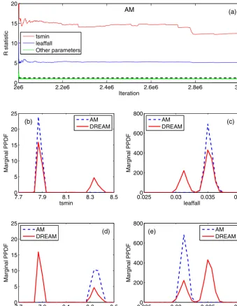
convergence. This setting facilitated the convergence of AM but resulted in AM false convergence to inaccurate PPDFs, leading to a relatively poor calibration and predictive per-formance. We implemented another AM simulation here for further examination. In this new simulation, we constructed two independent AM chains; both chains initializedC0using the DREAM samplesafterconvergence, but one chain only
used tsmin samples around its left mode and leaffall
sam-ples around its right mode, and the other chain usedtsmin
samples around its right mode andleaffallsamples around its left mode. Each chain evolved 3 000 000 iterations, and for the last 1 000 000 iterations the convergence diagnostic
ˆ
R values were calculated and shown in Fig. 9a. The figure indicates that most parameters haveRˆ less than the thresh-old of 1.2 except parameterstsminandleaffall, whose values are far above 1.2 and no signs show that they are going sig-nificantly smaller in the following 1 000 000 iterations. This suggests that the two chains converged to different optima for these two parameters. We then estimated PPDFs using the last 500 000 samples from each chain respectively. The results fortsminandleaffallare shown in Fig. 9b–e. The fig-ures illustrate that the samples from one AM chain can only identify one mode, and this mode is consistent with the sam-ples used to construct the initial covariance matrixC0.
As a single-chain sampler, it is conceptually possible for AM to become trapped in a single mode (Jeremiah et al., 2011). Consider a distribution with two far-separated modes and assume that the chain is initialized near one of the two modes (both samples initialization and proposal covariance initialization). At the beginning of the sampling, AM will explore the area around the mode where it is initialized and start identifying the first mode. Since the candidate samples generated by the Gaussian proposal have higher Metropolis ratios (Eq. 2) in the nearby area than in the far-away regions of the identified mode, the chain is hardly to move to the other mode. When the Gaussian proposal covariance matrix Ct begins to update, the chance of the chain jumping to the
other mode depends on the relative scale of the proposal co-variance and the distance between the two modes. When the modes’ separation exceeds the range of the proposal, AM is less likely to escape the identified local mode.
2e60 2.2e6 2.4e6 2.6e6 2.8e6 3e6 5
10 15 20
R statistic
Iteration
AM (a)
tsmin leaffall
Other parameters
7.7 7.9 8.1 8.3 8.5
0 5 10 15 20 25
Marginal PPDF
tsmin
(b) AM
DREAM
0.0250 0.03 0.035 0.04
200 400 600 800
Marginal PPDF
leaffall
(c)
AM DREAM
7.7 7.9 8.1 8.3 8.5
0 5 10 15 20 25
Marginal PPDF
tsmin
(d)
AM DREAM
0.0250 0.03 0.035 0.04
200 400 600 800
Marginal PPDF
leaffall
(e) AM
[image:14.612.127.467.68.507.2]DREAM
Figure 9.Results of two independent chains of AM with the initial covariance matrix constructed using the converged DREAM samples. TheRˆstatistic in(a)suggests that different AM chains converged to differenttsminandleaffallvalues. One chain captures(b)the left mode
oftsminand(c)the corresponding right mode ofleaffall, and the other chain identifies(d)the right mode oftsminand(e)the corresponding
left mode ofleaffall. No single AM chain can capture all the modes of the two parameters within a reasonable number of MCMC iterations.
the other 19 parameters from the two chains are close to each other and both similar to the DREAM results. This finding once again shows the reasonable existence of the two sep-arated modes and their equivalent importance. With an im-proved initialization ofC0in the new simulation, the perfor-mance of AM also improved as it can accurately simulate unimodal PPDFs and capture one mode for the multimodal PPDFs. This investigation suggests that for AM an appro-priate initialization of its Gaussian proposal has a signifi-cant impact on its performance. We made several test runs of AM, and only when we initializedC0using the complete
set of converged DREAM samples was AM able to produce PPDFs similar to the ones resulted from DREAM with iden-tifying all the possible optima. However, the information of a reasonableC0in practice is either unavailable or very com-putationally expensive to obtain.
4 Discussion
−10 −5 0 5 10 −8
−6 −4 −2 0 2 4 6 8
Simulated NEE
Residuals
(a)
−100 −5 0 5 10
0.1 0.2 0.3 0.4
Residuals
Density
(b)
Assumed PDF Actual PDF
0 10 20 30 40
−0.2 0 0.2 0.4 0.6 0.8
Lags (d)
Partial autocorrelation
[image:15.612.101.495.67.192.2](c)
Figure 10. Residual analysis of the calibration using Gaussian likelihood with heteroscedastic anduncorrelatederrors:(a)residuals vs. simulated NEE;(b)assumed and actual probability density functions of residuals; and(c)partial autocorrelation coefficients of residuals with 95 % significance levels (black dashed lines).
study, we assumed a heteroscedastic, uncorrelated, Gaussian error model. However, this simplistic assumption may not be realistic for complex TEMs. In this section, we examine whether the assumed error model provides an accurate repre-sentation of residuals between the simulated and observed NEEs. If the assumptions are not satisfied, we consider a more flexible error model and investigate the influence of the corresponding likelihood function on parameter estimation and model performance.
Figure 10 presents results of residual analysis based on the heteroscedastic, uncorrelated, Gaussian assumption. The plot of residuals versus simulated NEE in Fig. 10a justifies the assumption of heteroscedastic variances; the density plot of residuals in Fig. 10b justifies the assumption of normal-ity, but the autocorrelation plot of residuals in Fig. 10c indi-cates that the errors are significantly correlated at a lag of 4, which violates the independence assumption. This violation has been reported in several time-series data models, such as the TEM in Ricciuto et al. (2008), the rainfall–runoff model in Feyen et al. (2007), and the groundwater reactive transport model in Lu et al. (2013). The correlated errors are likely to be observed in models where systematic model errors exist like the DALEC model in this study.
According to the residual analysis, we consider a het-eroscedastic,correlated, Gaussian error model and construct the likelihood function correspondingly. Similar to Schoups and Vrugt (2010), the heteroscedasticity was explicitly ac-counted for using a linear modelσt=σ0+σ1Et, whereσt
represents the error standard deviation,σ0andσ1are param-eters to be inferred from the data andEt is the mean value of
NEE. The correlation was simulated by thepth-order autore-gressive model AR(p). This new error model adds six extra parameters besides the original 21 TEM parameters, where parametersσ0andσ1are related to the heteroscedastic error model and φ1,φ2, φ3, andφ4 are from the AR(4) correla-tion model. We set up a DREAM simulacorrela-tion to estimate the PPDFs of the 27 parameters and compared the results with those using the uncorrelated error assumption.
Figure 11 indicates that the six error model parameters are well identified in current parameter ranges. The het-eroscedastic parametersσ0andσ1approach 1 and 0, respec-tively, which suggests that a constant variance may be rea-sonable. This finding contradicts what we usually assumed – that the data errors are heteroscedastic. The reason for this could be the epistemic error or forcing data errors. Alterna-tively, an extended prior distribution ofσ0andσ1may give different results. More work is needed to find out the underly-ing reasons. The nonzeroφ1,φ2,φ3, andφ4values indicate that a AR(4) correlation model is necessary. This new het-eroscedastic, correlated, Gaussian error model is appropriate as the resulted residuals demonstrate consistent features with the a priori assumptions. As it is shown in Fig. 12, the resid-uals are randomly distributed around the zero line (Fig. 12a), normally distributed as assumed (Fig. 12b), and no longer correlated after considering the AR(4) model (Fig. 12c).
0.990 0.995 1 100
200 300 400
0
PPDF of error model parameters
0 2 4 6
x 10−4
0 1000 2000 3000 4000 5000 6000
1
MAP estimate
0.3 0.35 0.4
0 5 10 15 20 25 30 35
1
0.06 0.08 0.1 0.12 0.14 0.16 0.180
5 10 15 20 25 30
2
PPDF of error model parameters
0.050 0.1 0.15 0.2
5 10 15 20 25 30
3
0.06 0.08 0.1 0.12 0.14 0.16 0.180
5 10 15 20 25 30
[image:16.612.101.490.68.345.2]4
Figure 11.Estimated posterior probability density functions (PPDFs) of the six error model parameters.
−10 −5 0 5 10
−8 −6 −4 −2 0 2 4 6 8
Simulated NEE
Residuals
(a)
−50 0 5
0.2 0.4 0.6 0.8 1
Residuals
Density
(b)
Assumed PDF Actual PDF
0 10 20 30 40
−0.2 0 0.2 0.4 0.6 0.8
Lags (d)
Partial autocorrelation
(c)
Figure 12.Residual analysis of the calibration using Gaussian likelihood with heteroscedastic andcorrelatederrors:(a)residuals vs. sim-ulated NEE;(b)assumed and actual probability density functions of residuals; and(c)partial autocorrelation coefficients of residuals with 95 % significance levels (black dashed lines).
study shows that these two parameters have wide confidence intervals that almost occupy the entire allowable ranges, in-dicating that the NEE data should provide little information about these parameters. The tight uncertainty bounds result-ing from the uncorrelated error assumption are likely unre-alistic and could contribute to overconfidence in model pre-dictions. The appropriate correlated error assumption con-siders the error correlation that reduces the data informa-tion for calibrating parameters, thus alleviating the problem of underestimation of parameter uncertainties. The underes-timation of parameter uncertainty using uncorrelated error model was also reported in Ricciuto et al. (2008), Schoups
and Vrugt (2010), and Lu et al. (2013). Moreover, Fig. 13 in-dicates that some parameters have similar PPDFs for the two different likelihood choices, such asgdd_min andq10_mr. Those parameters that are not much affected by the model error assumptions should, in theory, be reasonably well de-termined in parameter estimation. And according to Safta et al. (2015), these less changed parameters are indeed sensitive parameters.
[image:16.612.100.497.386.510.2]30 40 50 0 0.05 0.1 0.15 gdd_min Marginal PPDF
160 180 200 220 0 0.05 0.1 gdd_max 2 2.2 0 20 40 60 80 laimax
6 7 8
0 5 10 15
tsmin
Uncorrelated likelihood Correlated likelihood
0.020 0.04 0.06
100 200 300 400
Leaffall
8 10 12
0 0.5 1
nue
0.050 0.1
20 40 60
rg_frac
6 8 10
x 10−3
0 500 1000 1500 br_mr Marginal PPDF 1 1.05 0 50 100
q10_mr 0.7 0.8 0.9
0 10 20
astem 5 10 x 1015−4
0 2000 4000
troot 5 10 x 1015−5
0 5 10
x 104
tstem 2 3 4
0 1 2
q10_hr 4.4 4.6 4.8 5 5.2 5.4x 10⁻³
0 2000 4000
br_lit
3 4 5
x 10−5
0 1 2 3
x 105
br_som
Marginal PPDF
2 4 6
x 10−3
0 200 400 600 800
dr 100 150
0 0.05 0.1
lma 5000 10 000 15 000
0 2 4
6x 10
−4
stemc_init 100 200 300
0 0.1 0.2 0.3
rootc_init 500 1000
0 0.005 0.01
litc_init 3000 7000 11 000
0 0.5 1 1.5
x 10−3
[image:17.612.52.544.67.270.2]somc_init
Figure 13.Estimated marginal posterior probability density functions (PPDFs) of the 21 TEM parameters using the uncorrelated and corre-lated Gaussian likelihoods.
1 6 11 16 21 26 31
−4 −2 0 2 4 6 October 1995 NEE Observation
Uncorrelated likelihood (RMSE = 0.9) Correlated likelihood (RMSE = 0.9)
Figure 14. Simulated NEE values based on the MAP estimates from the uncorrelated and correlated Gaussian likelihoods in Oc-tober 1995.
similar, the simulations on a single day are different. This is not surprising, as MCMC is a Bayesian calibration and the calibration results depend on the choice of the likelihood function, mainly the assumptions of the error model. In this study, the heteroscedastic, correlated, Gaussian error model is more reasonable than the uncorrelated one.
5 Conclusions
In this work, we apply two advanced MCMC algorithms, AM and DREAM, in the Bayesian calibration of the terres-trial ecosystem model DALEC. In both synthetic and real-data studies, we found that AM is sensitive to the algorithm
initializations. When it starts with a proper initialization, through prior information or some test runs or even some dimension-reduction strategies, AM can produce reasonable approximation of the parameter posterior distributions. How-ever, AM still shows some difficulties in sampling multi-modal distributions with the Gaussian proposal. By com-parison, DREAM’s performance does not depend on initial-ization of the algorithm and can fast converge to the high-dimensional and multimodal distributions. Thus, DREAM is particularly suitable to calibrate complex terrestrial ecosys-tem models, where the uncertain parameter size is usually large and existence of local optima is always a concern. The application indicates that, compared to AM, DREAM can accurately simulate the posterior distributions of the model parameters, resulting in a better model fit, superior predic-tive performance, and perhaps identifying structural errors or process differences between the model and ecosystem from which observations were used for calibration.
In Bayesian calibration, the choice of likelihood function plays an important role in parameter estimation. In this effort, we justify the assumptions of error model used in construct-ing the likelihood function and find that a heteroscedastic, correlated, Gaussian error model is reasonable for this prob-lem as supported by the residual analysis.
Data availability. The NEE observation data used in this study are
available from Oak Ridge National Laboratory Distributed Active Archive Center (https://doi.org/10.3334/ORNLDAAC/1183).
Competing interests. The authors declare that they have no conflict
[image:17.612.67.267.323.493.2]