Volume 2, Issue 6, December 2014
Abstract— In this paper, emphasis has been given to compress ECG data using Turning Point Algorithm which compresses the ECG data in the ratio 2:1. For this we have acquired different ECG signals using POLYPARA system and MIT-BIH database and using MATLAB software we implemented the algorithm and obtain the results for different ECG signals and found that the Turning Point Algorithm produces a fixed compression ratio of 2:1.
Index Terms—Compression ratio, ECG Compression, MIT-BIH database, Turning Point Algorithm.
I. INTRODUCTION
An electrocardiogram is a recording of electrical activity of heart over the time produced by an electrocardiograph. Electrical impulses originate in the sinoatrial node of the heart and travel through the heart muscle where they impart electrical initiation of systole or contraction of the heart [1].The electrical waves can be measured at selectively placed electrodes (electrical contacts) on the skin. Electrodes on different sides of the heart measure the activity of different parts of the heart muscle. An ECG displays the voltage between pairs of these electrodes, and the muscle activity that they measure, from different directions, also understood as vectors. After acquiring the signal, different ECG signal compression techniques using MATLAB software are implemented by several researchers [2-6].
A typical computerized medical signal processing system acquires a large amount of data that is difficult to store and transmit. We need a way to reduce the data storage space while preserving the significant clinical content for signal reconstruction. This process is called data compression.
A data reduction algorithm seeks to minimize the number of code bits stored by reducing the redundancy present in the original signal. We obtain the reduction ratio by dividing the number of bits of the original signal by the number saved in the compressed signal. We generally desire a high reduction ratio but caution against using this parameter as the sole basis of comparison among data reduction algorithms. Factors such as bandwidth, sampling
frequency, and precision of the original data generally have considerable effect on the reduction ratio. A data reduction algorithm must also represent the data with acceptable fidelity. In biomedical data reduction, we
usually determine the clinical acceptability of the reconstructed signal through visual inspection. We also measure the residual, that is, the difference between the reconstructed signal and the original signal. Such a numerical measure is the percent root-mean-square difference, PRD, and is mathematically given by
Where n is the number of samples and xorg and xrec are samples of the original and reconstructed data sequences. A
lossless data reduction algorithm produces zero residual, and the reconstructed signal exactly replicates the original signal. However, clinically acceptable quality is neither guaranteed by a low nonzero residual nor ruled out by a high numerical residual. For example, a data reduction algorithm for an ECG recording may eliminate
ECG Data Compression using Turning Point
Algorithm
Muzaffar Saba Anjum and Dr. Monisha Chakraborty
*Final year Student of Master of Biomedical Engineering, School of Bio-Science & Engineering
Jadavpur University, Kolkata-700032,
These techniques generally retain samples that contain important information about the signal and discard the rest. Since they produce nonzero residuals, they are lossy algorithms. In the second class of techniques based on Huffman coding, variable length code words are assigned to a given quantized data sequence according to frequency of occurrence. A predictive algorithm is normally used together with Huffman coding to further reduce data redundancy by examining a successive number of neighboring samples [7].
II. METHODS
The turning point (TP) algorithm was originally developed to reduce the sampling frequency of an ECG signal from 200 to 100 Hz .The algorithm developed from the observation that, except for QRS complexes with large amplitudes and slopes, a sampling rate of 100 Hz is adequate.TP is based on the concept that ECG signals are normally oversampled at four or five times faster than the highest frequency present. For example, an ECG used in monitoring may have a bandwidth of 50 Hz and be sampled at 200 sps in order to easily visualize the higher-frequency attributes of the QRS complex. Sampling theory tells us that we can sample such a signal at 100 sps. TP provides a way to reduce the effective sampling rate by half to 100 sps by selectively saving important signal points (i.e., the peaks and valleys or turning points).This is the reason behind selecting Turning Point (TP) over other direct data compression techniques.
The algorithm processes three data points at a time. It stores the first sample point and assigns it as the reference point X0. The next two consecutive points become X1 and X2. The algorithm retains either X1 or X2, depending on
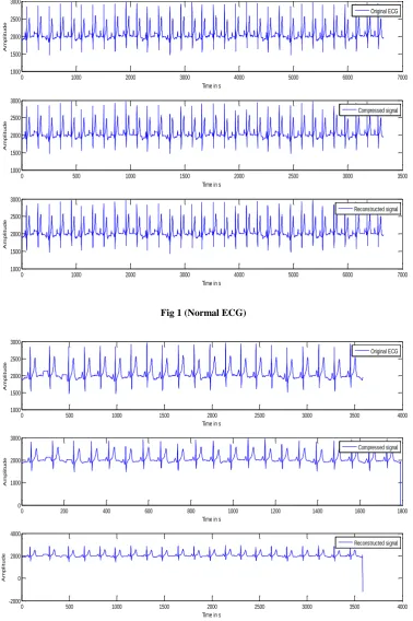
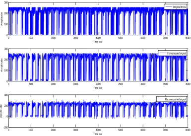
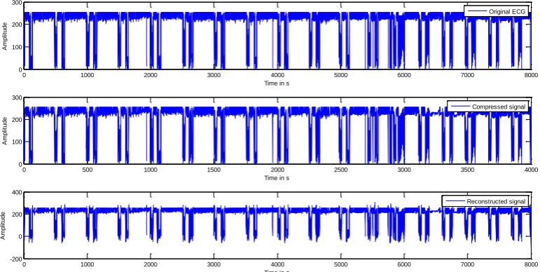
which point preserves the turning point (i.e., slope change) of the original signal. The TP Algorithm produces a fixed compression ratio of 2:1 and the reconstructed signal resembles the original signal with some distortions. The steps of Turning Point are as follows:
i.Acquire the ECG signal.
ii. Take the first three samples and check for the condition as mentioned below:
(X1-X0)*(X2-X1)<0
(or) (X1-X0)*(X2-X1)>0
iii. If the above condition-1 is correct then X1 is stored else X2 is stored.
iv. Reconstructing the compressed signal.
The compression ratio of Turning point algorithm is 2:1, if higher compression is required then the same algorithm can be implemented on the already compressed signal so that it is further compressed to a ratio of 4:1. But after the 2nd compression, the required data in the signal may be lost since the signal is overlapped on one another.
Therefore, TP algorithm is limited to compression ratio of 4:1. TP algorithm can be applied on the already compressed data to increase the compression ratio to 4:1.
III. REQUIREMENTS
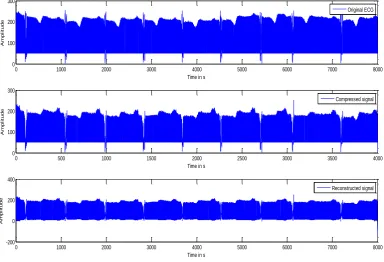
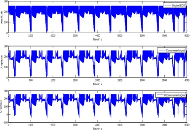
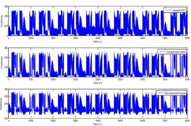
a. Acquisition of ECG Signals: The normal ECG signals are acquired using POLYPARA System. The diseased ECG signals are collected from MIT-BIH database [8].
b.MATLAB Software: MATLAB Version R2009b is used for implementing the programs.
c. PC configuration with 2 GB RAM, 320 GB HARD DISK and 2 GHz Intel Processor.
IV. RESULTS
Volume 2, Issue 6, December 2014
0 1000 2000 3000 4000 5000 6000 7000
1000 1500 2000 2500 3000
Time in s
A
m
p
li
tu
d
e
Original ECG
0 500 1000 1500 2000 2500 3000 3500
1000 1500 2000 2500 3000
Time in s
A
m
p
li
tu
d
e
Compressed signal
0 1000 2000 3000 4000 5000 6000 7000
1000 1500 2000 2500 3000
Time in s
A
m
p
li
tu
d
e
Reconstructed signal
Fig 1 (Normal ECG)
0 500 1000 1500 2000 2500 3000 3500 4000
1000 1500 2000 2500 3000
Time in s
A
m
p
li
tu
d
e
Original ECG
0 200 400 600 800 1000 1200 1400 1600 1800
0 1000 2000 3000
Time in s
A
m
p
li
tu
d
e
Compressed signal
-2000 0 2000 4000
A
m
p
li
tu
d
e
0 1000 2000 3000 4000 5000 6000 7000 8000 0
100 200 300
Time in s
A
m
p
li
tu
d
e
Original ECG
0 500 1000 1500 2000 2500 3000 3500 4000
0 100 200 300
Time in s
A
m
p
li
tu
d
e
Compressed signal
0 1000 2000 3000 4000 5000 6000 7000 8000
-200 0 200 400
Time in s
A
m
p
li
tu
d
e
Reconstructed signal
Fig 3 (Arrhythmia ECG )
0 1000 2000 3000 4000 5000 6000 7000 8000
0 100 200 300
Time in s
A
m
p
li
tu
d
e
Original ECG
0 500 1000 1500 2000 2500 3000 3500 4000
0 100 200 300
Time in s
A
m
p
li
tu
d
e
Compressed signal
0 1000 2000 3000 4000 5000 6000 7000 8000
-100 0 100 200 300
Time in s
A
m
p
li
tu
d
e
Reconstructed signal
Volume 2, Issue 6, December 2014
0 1000 2000 3000 4000 5000 6000 7000 8000
0 100 200 300
Time in s
A
m
p
li
tu
d
e
Original ECG
0 500 1000 1500 2000 2500 3000 3500 4000
0 100 200 300
Time in s
A
m
p
li
tu
d
e
Compressed signal
0 1000 2000 3000 4000 5000 6000 7000 8000
-100 0 100 200 300
Time in s
A
m
p
li
tu
d
e
Reconstructed signal
Fig 5 (Congestive Heart Failure ECG)
0 1000 2000 3000 4000 5000 6000 7000 8000
100 150 200 250 300
Time in s
A
m
p
li
tu
d
e
Original ECG
0 500 1000 1500 2000 2500 3000 3500 4000
0 100 200 300
Time in s
A
m
p
li
tu
d
e
Compressed signal
-200 0 200 400
A
m
p
li
tu
d
e
0 1000 2000 3000 4000 5000 6000 7000 8000 0
100 200 300
Time in s
A
m
p
li
tu
d
e
Original ECG
0 500 1000 1500 2000 2500 3000 3500 4000
0 100 200 300
Time in s
A
m
p
li
tu
d
e
Compressed signal
0 1000 2000 3000 4000 5000 6000 7000 8000
-100 0 100 200 300
Time in s
A
m
p
li
tu
d
e
Reconstructed signal
Fig 7 (Malignant Ventricular Arrhythmia ECG)
0 1000 2000 3000 4000 5000 6000 7000 8000
0 100 200 300
Time in s
A
m
p
li
tu
d
e
Original ECG
0 500 1000 1500 2000 2500 3000 3500 4000
0 100 200 300
Time in s
A
m
p
li
tu
d
e
Compressed signal
0 1000 2000 3000 4000 5000 6000 7000 8000
-100 0 100 200 300
Time in s
A
m
p
li
tu
d
e
Reconstructed signal
Volume 2, Issue 6, December 2014
0 1000 2000 3000 4000 5000 6000 7000 8000
0 100 200 300
Time in s
A
m
p
li
tu
d
e
Original ECG
0 500 1000 1500 2000 2500 3000 3500 4000
0 100 200 300
Time in s
A
m
p
li
tu
d
e
Compressed signal
0 1000 2000 3000 4000 5000 6000 7000 8000
-200 0 200 400
Time in s
A
m
p
li
tu
d
e
Reconstructed signal
Fig 9 (Normal Sinus Rhythm ECG)
0 1000 2000 3000 4000 5000 6000 7000 8000
0 100 200 300
Time in s
A
m
p
li
tu
d
e
Original ECG
0 500 1000 1500 2000 2500 3000 3500 4000
0 100 200 300
Time in s
A
m
p
li
tu
d
e
Compressed signal
0 200 400
A
m
p
li
tu
d
e
0 1000 2000 3000 4000 5000 6000 7000 8000 0
100 200
Time in s
A
m
p
lit
u
d
e
Original ECG
0 500 1000 1500 2000 2500 3000 3500 4000
0 100 200 300
Time in s
A
m
p
lit
u
d
e
Compressed signal
0 1000 2000 3000 4000 5000 6000 7000 8000
-200 0 200 400
Time in s
A
m
p
lit
u
d
e
Reconstructed signal
Fig 11 (Supra-Ventricular Arrhythmia ECG)
0 1000 2000 3000 4000 5000 6000 7000 8000
0 100 200 300
Time in s
A
m
p
lit
u
d
e
Original ECG
0 500 1000 1500 2000 2500 3000 3500 4000
0 100 200 300
Time in s
A
m
p
lit
u
d
e
Compressed signal
0 1000 2000 3000 4000 5000 6000 7000 8000
-200 0 200 400
Time in s
A
m
p
lit
u
d
e
Reconstructed signal
Fig 12 (Supra-Ventricular Arrhythmia ECG)
V. CONCLUSION
In all the results of normal and diseased ECG data the compression ratio is 2:1. Moreover from the results it is observed that the morphology of the compressed signal is not getting deteriorated. This shows that the Turning Point Algorithm for ECG Compression always produces a reduction ratio of 2:1 without much distortions in the reconstructed signal and this satisfied our goal of using Turning Point Algorithm. If we want to increase the compression ratio the same algorithm can be applied on the compressed signal.
ACKNOWLEDGMENT
Volume 2, Issue 6, December 2014 REFERENCES
[1] S. Jalaleddine, C. Hutchens, R. Stratan, and W. A. Co-berly, (1990) ECG data compression techniques-a unified approach, IEEE Trans. Biomed. Eng., 37, 329-343.
[2] J. R. Cox, F. M. Nolle, H. A. Fozzard, and G. C. Oliver, (1968) AZTEC, a preprocessing program for real time ECG
rhythm analysis, IEEE Trans. Biomed. Eng., BME-15, 129-129.
[3] D. C. Reddy, (2007) biomedical signal processing-principles and techniques, 254-300, Tata McGraw-Hill, Third reprint.
[4] J. L. Simmlow, Biosignal and biomedical image processing- MATLAB based applications, 4-29.
[5] V. Kumar, S. C. Saxena, and V. K. Giri, (2006) direct data compression of ECG signal for telemedicine, ICSS, 10, 45-63.
[6] W.C.Mueller Arrhythmia detection program for an ambulatory ECG monitor, “Biomed. Sci. Instrument., vol. 14, pp. 81-85.
[7] S. K. Mukhopadhyay, M. Mitra, S. Mitra, “A lossless ECG data compression technique using ASCII character encoding”,
Computers and Electrical Engineering 37 (2011) 486–497.