ISSN: 2008-6822 (electronic)
https://dx.doi.org/10.22075/IJNAA.2019.4060
Adaptive fuzzy sliding mode and indirect
radial-basis-function neural network controller for
trajectory tracking control of a car-like robot
Masoud Shirzadeha, Abdollah Amirkhanib,*, Mohammad H. Shojaeefardb, Hamid Behroozic
aDepartment of Electrical Engineering, Amirkabir University of Technology, Tehran 15875-4413
bDepartment of Automotive Engineering, Iran University of Science and Technology, Tehran 16846-13114, Iran cDepartment of Electrical Engineering, Sharif University of Technology, Tehran, Iran
(Communicated by M.B. Ghaemi)
Abstract
The ever-growing use of various vehicles for transportation, on the one hand, and the statistics of soaring road accidents resulting from human error, on the other hand, reminds us of the necessity to conduct more extensive research on the design, manufacturing and control of driver-less intelligent vehicles. For the automatic control of an autonomous vehicle, we need its dynamic model, which, due to the existing uncertainties, the un-modeled dynamics and the performed simplifications, is impossible to determine exactly. Add to this, the external disturbances that exist on the movement path. In this paper, two adaptive controllers have been proposed for tracking the trajectory of a car-like robot. The first controller includes an indirect radial-basis-function neural network whose parameters are updated online via gradient descent. The second controller is adaptively updated online by means of fuzzy logic. The proposed controller includes a nonlinear robust section that uses the sliding mode method and a fuzzy logic section that updates some of the nonlinear control parameters online. The fuzzy logic system has been designed to deal with the chattering problem in the controller of car-like robot. In both controllers, the parameters have been determined by means of genetic algorithm. The obtained results indicate that even with the consideration of un-ideal effects such as uncertainties and external disturbances, the proposed controller has been able to perform successfully.
Keywords: dynamic model, trajectory tracking, car-like robot, sliding mode, fuzzy logic system.
2010 MSC: 93C42.
∗Corresponding author
Email address: [email protected](Abdollah Amirkhanib,*)
1. Introduction
Vehicles as means of transportation are considered a necessity in today’s world. However, the use of vehicles has resulted in detrimental outcomes, as well. Road accidents involving automotive have taken the lives of 1.3 million individuals around the world in 2015 and about 1.4 million in 2016. According to the World Health Organization, fatal driving accidents rank as the 10th cause of death in the world [1]. Driver error is the cause of 72% of car accidents [2]. With the rapid advancement of artificial intelligence and car technology, autonomous vehicles are expected to take the pressure and stress of driving off the drivers and thus improve their workload and safety. Here, we have focused on the control system of an autonomous vehicle, and tried to present a controller for a basic model of such a car. Many of the previous works have introduced tracking controllers for driver-less automotive. Researchers initially designed motion controllers for these cars based on their kinematic model [3] and then started designing tracking controllers using the dynamic model. A simple fuzzy proportionalintegralderivative (PID) controller for the kinematic model of a car-like robot has been presented in [4]. Some researchers have designed kinematic model-based controllers while considering the skidding and slipping of car tires [5]. Using the virtual vehicle method, several articles have presented controllers for car-like robots based on their dynamic models [6]. The trajectory tracking of autonomous vehicles using the predictive control method has been discussed in [7]. In this study, the front wheel angle has been used in the control scheme. A path-following scheme for an autonomous four-wheeler using the combination of sliding mode and feedback control, along with the control of yaw moment, has been presented in [8] for the direct control of the car wheel. Numerous research works have been conducted on the lateral motion control of autonomous vehicles at the Stanford University dynamic design lab [9]. It is always challenging to determine the exact kinematic and dynamic models, and the uncertainties in these models cannot be avoided. In this regard, many researchers have presented adaptive and robust controllers for dealing with the issue of path tracking in wheeled mobile robots [10, 11]. Due to the existence of parametric and non-parametric uncertainties in system models and also the existence of non-holonomic constraints, the designing of output feedback controllers is a challenging task. Besides, the separation principle cannot be easily applied in this case. Both the trajectory-tracking and path-following problems have their own particular complexities when it comes to the kinematic model of car-like moving robots, which happens to be non-holonomic. The uncertainties associated with parametric modeling and unknown external disturbances constitute a significant concern in the development of advanced controllers for uncrewed vehicles. The unknown external disturbances may be caused by changing driving conditions. An adaptive neural controller for controlling the movement of an autonomous vehicle has been presented in this paper. The target of this work is to design an indirect adaptive output feedback controller by using an artificial neural network (NN) and considering model uncertainties and external disturbances. The network used in this indirect controller is a type of NN with radial basis functions (RBFs).
function gains are adaptively modified by applying fuzzy logic. In addition to using the fuzzy logic system (FLS), the other constant parameters in the designed nonlinear controller are determined to employ GA. This paper has been organized as follows: The dynamic model of the car-like robot has been given in Section 2. IANC, along with its kinematic control and stability analysis, have been presented in Section 3. The adaptive sliding mode nonlinear controller, the stability analysis, and the FLS have been presented in Section 4. Simulation results and the conclusion have been presented in Section 5 and Section 6, respectively.
2. The dynamic model of the car-like robot
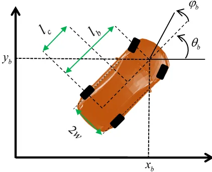
Consider the car-like robot in Figure 1. The configuration of variables is presented asq:= (xb, yb, θb, ϕb)T;
where (xb, yb) are the Cartesian coordinates of the midpoint between two rear wheels,θb is the angle
of car body relative to the x-axis, and ϕb is the control wheel angle. Assuming that the rear and
front tires do not skid on the ground, the system constraints are written as
A(q)q˙ =
−sin (θb+φb) cos (θb +φb) 0 0 −sin (θb) cos (θb) −lb 0
˙
q= 0 (2.1)
where lb is the distance between the axles of front and rear wheels. The kinematic model of the
car-like robot is obtained as
˙
q =
cos (θb) sin (θb) tan(lbϕb) 0
0 0 0 1
| {z }
ST
T
vb
ωb
| {z } V
(2.2)
ωb denotes the angular velocity of the front wheels and vb is the car velocity. According to the
Lagrange method, the dynamic equation of the system is derived as (see [12]):
m 0 Icsin (θb) 0
0 m −Iccos (θb) 0
Icsin (θb) −Iccos (θb) Ib Iw
0 0 Iw Iw
| {z }
M ¨ q+
0 0 −Icθ˙bcos (θb) 0
0 0 −Icθ˙bsin (θb) 0
0 0 0 0
0 0 0 0
| {z }
V ˙ q = Tx Ty Tθ Tϕ
| {z }
T
+τd+AT
λ1
λ2
| {z } Λ
(2.3)
wherem :=Mb+4mw,Iw := 2Iwzz,Ic:= ((lb−lc)Mb+ 2lbmw) andIb :=Mb(lb−lc)
2
+4W2mw+
2lb2mw+Ibzz+ 4Iwzz. Tis the vector of forces and moments applied to the system in the generalized
coordinates q, and it is related to the vector of moments applied to the robot as follows:
Tx Ty Tθ Tϕ
| {z }
T =
cos (θb) 0
sin (θb) 0
lbcos (ϕb) sin (ϕb) 0
0 1
| {z }
B
τ1
τ2
| {z }
τ
Using the pseudo-inverse method, the inverse of Eq. (2.4) is obtained as
τ1
τ2
| {z }
τ
=
−cos(θb)
b
−sin(θb)
b
−lbcos(ϕb) sin(ϕb)
b 0
0 0 0 1
| {z }
B†
Tx
Ty
Tθ
Tϕ
| {z }
T
, b :=lb2 cos4(ϕb)−cos2(ϕb)
−1
(2.5)
In Eq. (2.3),Λ is the Lagrange coefficients,τdis the vector of disturbing forces, τ1 is the moment
applied to the rear wheels, is the moment applied to the control wheel, is the wheel radius, is the wheel mass,Iwzz is the wheel moment of inertia about the z-axis passing through the wheel centroid, Mb is the car body mass, and Ibzz is the moment of inertia of car body about the z-axis passing
through the car bodys center of mass.
Figure 1: The car-like robot along with the relevant coordinate frames.
The term STAT=0 can be used to eliminate Λ and A from the vehicles dynamic equation [8].
The reduced form of the cars equation is expressed as follows:
MxV˙ +VxV =Bxτ+τx,Mx:=STMS= [mij],Vx :=ST(M ˙S+VS) = [vij],
τx:=STτd,Bx :=STB= [bij], i= 1,2, j = 1,2
(2.6)
In order to obtain the Lagrange coefficients, Eq. (2.3) and the time-derivative of Eq. (2.1) are simultaneously solved, as follows:
τ Λ
=AM−1B AM−1ATT
AM−1B AM−1AT
∗
AM−1B AM−1ATT −1
−A˙q˙+AM−1Vq˙ (2.7)
3. Indirect RBF neural network controller by means of genetic algorithm
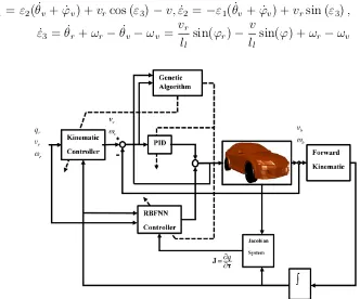
In this section, by using an RBFNN, an indirect adaptive controller is designed for tracking the trajectory of the car-like robot. The general structure of this controller is presented in Figure 2. A car model designed in the MapleSim has also been displayed in this figure [13]. The controller structure includes the kinematic controller section, the PID controller section, the IANC section, the section for determining system Jacobean, and the GA section. The reference path is considered as qr := (xr, yr, θr, ϕr)T. The goal for the controller is to bring error eq := qv−q down to zero.
First, the kinematic controller is designed. Suppose the variables of a virtual vehicle are in the form of qv := (xv, yv, θv, ϕv)
T
. By designing a kinematic controller based on the Lyapunov method, we intend to eventually obtain the values of vv and ωv, which are the linear and the angular velocities
of the virtual vehicle, respectively. To this end, we implement the procedure presented in [14] for a wheeled mobile robot. First, the generalized error in the local coordinate system is obtained as follows [14]:
ε= (ε1, ε2, ε3),
ε1
ε2
=
cos(θv+ϕv) sin(θv+ϕv) −sin(θv+ϕv) cos(θv+ϕv)
ex
ey
, ε3 =θr+ϕr−(θv+ϕv) (3.1)
The nonholonomic constraint for the car-like robot is expressed as ˙xbsin(θb)−y˙bcos(θb). By
considering this constraint, the kinematic model for error ε is obtained. ˙
ε1 =ε2( ˙θv + ˙ϕv) +vrcos (ε3)−v,ε˙2 =−ε1( ˙θv+ ˙ϕv) +vrsin (ε3),
˙
ε3 = ˙θr+ωr−θ˙v −ωv =
vr
ll
sin(ϕr)−
v ll
sin(ϕ) +ωr−ωv
(3.2)
Figure 2: The general structure of the RBFNN controller for the car-like robot.
To design our controller for system (3.2), a Lyapunov function [14] and [15] is selected as follows:
L1 =
k1
2(ε
2 1+ε
2 2) + 2
sinε3 2
2
(3.3) By taking the derivative of (3.3) and performing a series of mathematical operations, (vv, ωv) are
ωv =k1vrε2+k3sin (ε3) +ωr+
vr
ll
sin(ϕr)−
v ll
sin(ϕ), vv =vrcos (ε3) +k2ε1 (3.4)
Following the kinematic control of the vehicle, a controller is designed to get (vb, ωb)→ (vv, ωv).
The main advantage of the kinematic controller is its simplicity; because it only relies on the kinematic model. The designed controller has three constant gains with positive values. In this paper, GA has been employed to determine these gains.The structure of the adaptive neural controller has been considered such that its parameters are updated online in order to minimize the following cost function:
F1 =
1 2E
TE,E= (e
1, e2)T, e1 :=vb−vv, e2 :=ωb−ωv (3.5)
The network used in this scheme is a type of artificial NN with RBFs. In this paper, the NN undergoes a data-to-data form of training, and this process enables the control of the vehicle [16]. In the considered network, h= (h1, h2, ..., hN2)
T
denotes the vector of radial functions in the hidden layer [16]; and it is defined as:
hj = exp −
kx−cjk
2b2
j
2!
, j = 1, ..., N2 (3.6)
wherex= (x1, x2, ..., xN1)
T
is the RBFNNs input vector, cj = (c1j, c2j, ..., cN3)
T
are the centers of Gaussian functions,bj, j = 1, ..., N2 are the widths of Gaussian functions, w= [wij], i= 1, ..., N2, j =
1, ..., N3 are the weights of RBFNNs output layer, and y = wTh = (y1, ..., yN3)
T
is the RBFNNs output vector. The descending gradient method is employed to train the NN online. By using the descending gradient approach, the RBFNN updating laws are obtained as
∆wjk(t) = −η
∂F1
∂wjk
=ηαkhj,∆bj(t) =−η
∂F1
∂bj
=η(wα)jhjbj−3kx−cjk
2
, α=sign(J)E
∆cij(t) =−η
∂F1
∂cij
=η(wα)jhj(xi−cij)b−j2, i= 1, ..., N1, j = 1, ..., N2, k = 1, ..., N3
wjk(t+ ∆t) = wjk(t) + ∆wjk(t)
bj(t+ ∆t) = bj(t) + ∆bj(t)
cij(t+ ∆t) =cij(t) + ∆cij(t)
(3.7)
where 0< η <1 is the updating rate of the NN parameters. J=∂q/∂τ is the systems Jacobean, which is expressed as the sensitivity of system output to input [16]. The systems Jacobean is obtained from the reduced equations of the system, as follows [17].
˙
V =M−x1Bxτ −M−x1VxV →V = Z t
0
M−x1Bxτ dt0− Z t
0
M−x1VxV dt0 →
∂V ∂τ =
Z t
0
M−x1Bxdt0 = ∂vb ∂τ1 ∂vb ∂τ2 ∂ωb ∂τ1 ∂ωb ∂τ2
,J =
Z
S∂V ∂τdt
0
(3.8)
Only the sign of Jacobeansign(J) has been used in the equation for updating the NN parameters. The kinematic controller has a gain ofK= (k1, k3, k4), and the coefficients of the PID controller are:
Kp = diag([kp1, kp2]), Ki = diag([ki1, ki2]) and Kd = diag([kd1, kd2]). The NN also has parameters
such as w, c, b= (b1, ..., bN3)
T
GA can be an appropriate method for determining the values of the mentioned gains. GA can also be used for path programming in mobile robots [19]. In this paper, GA is employed to obtain the abovementioned constant values as well as the initial values of NN parameters. For this purpose, first, a cost function is defined as
F2 =
1
Nβ1
X
ETE+ 1
Nβ2
X
(qr−q) T
(qr−q) +
1
N
X
(β3|τ1|+β4|τ2|), N :=
F T
∆t (3.9)
In the above equation, β = (β1, β2, β3, β4) are the weights considered for each term of the cost
function, is the simulation time, and is the sampling time step. The steps taken for the implemen-tation of GA are as follows: Step 1: Generating and evaluating random populations. In this paper, every generated population is evaluated immediately; and by evaluation, we mean the calculation of cost function (Eq. (3.9)) for each part of the population. Step 2: Selecting the parents and cross-ing them over to produce the offsprcross-ing population. Step 3: Selectcross-ing the members of the offsprcross-ing population and creating the mutated population. Step 4: Combining the original population with their offspring and the mutated population and establishing a new original population. The newly created population will form the current generation. Step 5: If the algorithm termination conditions are not met, go back to Step 2. Step 6: End of algorithm. Several conditions can be considered as the algorithm termination conditions: 1) Reaching an acceptable predefined limit for solution (e.g., the tracking error falling below a specified value). 2) Elapse of a specific time duration or reaching a definite number of iterations; if the time spent for executing the iterations is greater than a spec-ified duration or the number of algorithm iterations is higher than a set value, stop executing the algorithm. 3) Elapse of a specific time duration or reaching a definite number of iterations without observing a significant improvement in the results.
In this paper, the second condition has been used for terminating the algorithm. The procedures for combining the three mentioned populations (Step 4) are as follows: if Npop is the number of
initial population members, after producing three main populations, the offspring and the mutations of these three populations are considered together and are arranged (in ascending order) according to the cost function (Eq. (3.9)). Then,Npop members are selected from the beginning of this arranged
population and considered as the current generation. In this paper, the parents for producing the offspring are selected randomly.
4. Fuzzy nonlinear adaptive sliding mode controller
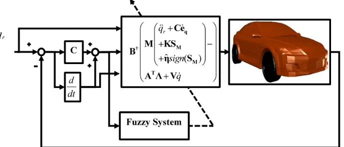
In this section, by employing the sliding mode and fuzzy logic techniques, a fuzzy sliding mode nonlinear controller will be designed. The structure of this controller, which has been displayed in Fig. 3, includes the sliding mode controller (SMC) section, the FLS and the GA section.
The controller error and the sliding mode manifolds are defined as
eq:=qr−q= (ex, ey, eθ, eϕ)T = (xr−x, yr−y, θr−θ, ϕr−ϕ)T (4.1)
SM :=Ceq+˙eq (4.2)
whereC:=diag(c1, c2, c3, c4) represents a definite positive diagonal matrix andSM:= (s1, s2, s3, s4)T
are the sliding mode manifolds. The SMC for the car-like robot has been designed as
Figure 3: The structure of the fuzzy adaptive nonlinear controller designed for the car-like robot.
The time derivatives of sliding mode manifoldsS˙Mhave been given in Eq. (4.4), and the reaching
rule has been presented in Eq. (4.5).
˙
SM =C ˙eq+¨eq =C ˙eq+ ¨qr−q¨=C ˙eq+ ¨qr−M−1 T+τd+ATΛ−Vq˙
(4.4)
˙
SM =−ηsign(SM)−KSM (4.5)
η := diag(η1, η2, η3, η4) and K := diag(k1, k2, k3, k4) in Eqs. (4.3) and (4.5) represent definite
positive diagonal matrices.
4.1. Stability analysis
To confirm the stability of the system and to ensure that error converges to zero, the Lyapunov function is considered as follows:
L2 =
1 2S
T
MSM (4.6)
By taking the derivative of Eq. (4.6) and substituting Eqs. (4.3)-(4.5) in it, we will have
˙
L=STMS˙M =STM C ˙eq+ ¨qr−M−1 T+τd+ATΛ−Vq˙
=STM −KSM−ηsign(SM)−M−1τd
(4.7) By assuming kM−1τdk ≤ Γ1 and kηk = Γ1 +kη1k (where Γ1 has a positive value), Eq. (4.7)
turns into Eq. (4.8).
˙
L=STM −KSM−ηsign(SM)−M−1τd
≤
− kKk kSMk2−(Γ1+kη1k)kSMk −STMM −1
τd≤ − kKk kSMk2− kη1k kSMk
(4.8) ˙
L is written as Eq. (4.8), and both sides of the equation are integrated. ˙
Z t
0
˙
Ldt0 =
Z t
0
− kKk kSMk2− kη1k kSMk
dt0 →L(0)−L(t) =
Z t
0
− kKk kSMk2− kη1k kSMk
dt0
→L(0) =L(t) +
Z t
0
kKk kSMk2+kη1k kSMk
dt0 →≥
Z t
0
kKk kSMk2+kη1k kSMk
dt0
(4.10)
lim
t→∞
Z t
0
kKk kSMk2+kη1k kSMk
dt0
≤L(0) <∞ (4.11) According to Barbalats Lemma [18], when t → ∞, then kKk kSMk2 + kη1k kSMk → 0; i.e.
lim
t→∞SM = 0; in other words, the surface of sliding mode SM is asymptotically stable. Thus, the
closed-loop errors converge to zero, and the stability of the closed-loop system is verified. In practice, for the prevention of chattering and for reducing the run time of the program (making the controller faster), function tanh (σisi) is used instead of functionsign(si); in this way, a uniformly ultimately
bounded stability is guaranteed.
4.2. Designing the fuzzy system
The fuzzy method utilized to reduce the fluctuations. In a SMC, the intensity of fluctuations depends on the gain of the sign function [20]; so by utilize the fuzzy system (FS) adaptively, the con-trol gain of the sign function is tuned according to the sliding surface (SS) and, thus, the amount of chattering is reduced [16]. Sliding occurs whensis˙i <0, i= 1, ...,4; if this condition is satisfied, when
system states reach the SS, they will be on the SS[20]. If system states are to reach the SS, the selec-tion of η:=diag(η1, η2, η3, η4) should eliminate the effects of uncertainties. There are two rules that
ensure the establishment of sliding condition [20]. Rule 1: ifsis˙i >0,ηi should be increased. Rule 2:
if sis˙i <0 then ηi should be decreased. From the two stated rules, the relationship between sis˙i and
˙
ηi, i= 1, ...,4 can be expressed as a FS.sis˙iand ˙ηi have been respectively chosen as the input and the
output of the FLS. For generating the gain of the sign function, the designed FS comprises 5 fuzzy rules as Rjf : IF sis˙i is Fj T hen ∆ηi is Gj,(j = 1, ...,5); where ˜F ={N B, N M, ZO, P M, P B}
de-notes the fuzzy set related to the input and ˜G ={N B, N M, ZO, P M, P B} is the fuzzy set related to the output. In fuzzy sets ˜F and ˜G, NB denotes negative big, NM represents negative medium, ZO indicates zero, PM means positive medium and PB is positive big.
The output of the FS shows the changes of sign function gain; therefore, by integrating the FS output, the estimated gain for the sign function is obtained according to Eq. (4.12) [20].
ˆ
ηi =gi
Z t
0
˙
ηidt0 (4.12)
where, gi, i = 1, ...,4 have constant values. By employing the FS presented, control gain ˆηi, i=
1, ...,4 varies adaptively and in a programmed way by means of fuzzy rules, and according to the changes of the SS and its time derivative. Hence, the adaptive, fuzzy, integrated, sliding mode control can be expressed as
T=M(¨qr+C ˙eq+KSM+ηsignˆ (SM))−ATΛ+Vq˙ (4.13)
where ηˆ:= diag(ˆη1,ηˆ2,ηˆ3,ηˆ4) indicates the time-variant switching control gain. For the inputs
of fuzzy systems to fall between -1 and 1, gains of fi, i = 1, ...,4 are considered at the inputs. Like
nonlinear fuzzy sliding mode adaptive controller. The selected cost function is Eq. (3.9), and the work procedure is similar to that explained in Section 3 for the IANC. After designing the controller, the simulation results will be presented in the next section.
5. Results
The following parameters and values have been used in the simulation: Mb = 2117 kg, mw =
28 kg, Iwzz = 0.78 kg.m
2, l
l = 2.787 m, lc = 1.487 m, Ibzz = 1925 kg.m
2, W = 0.7775 m, β =
(β1, β2, β3, β4) = (1,1,0.1,0.1), K = (40.71,33.3,67.78,49.44), C = (5.13,85.59,84.21,74.84), ∆t =
0.01 s and rw = 0.4 m. The inputs of RBFNN are: x = (q, qr,q,˙ q˙r) T
, and there are 10 neurons in the middle layer. The upper and lower bounds considered for control signal saturation are as follows: max(τ1) = 25,min(τ1) =−25,max(τ2) = 200,min(τ2) = −200.
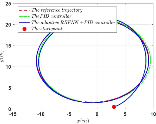
Figure 4: The trajectory of the car-like robot achieved by simulation under ideal conditions and by the IANC.
To evaluate the effects of disturbance and uncertainty, an external disturbance in the form ofτd=
(γ1sin(µ1t) exp (−b1|t−t1|), γ2sin(µ2t) exp (−b2|t−t2|))
T
and with numerical values of (b1, b2, t1, t2,
γ1, γ2, µ1, µ2) = (0.01,0.03,50s,120s,100,40,0.3,0.5) is applied to the system. The mean square error
(MSE) is defined as
M SE:= 1
F T
X
(qr−q)T(qr−q) (5.1)
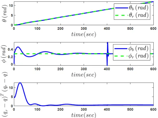
Figure 5: The trajectory of the car-like robot achieved by using the IANC and by considering the effects of uncertainty, external disturbance and control signal saturation.
To examine the robustness of the designed controller against control signal saturation, the effect of the saturation of control signals has also been considered in this simulation. Figures 5 and 6 reveal that the designed controller has been robust against the applied disturbance and has performed suc-cessfully. To explore the effect of car mass fluctuation on the performance of the designed controller, the mass of the vehicle has been increased by 20% at time t = 220s and reduced by 30% at time t = 400s.
Figure 6: The diagrams of car angle and error norm versus time obtained by considering the effects of uncertainty, external disturbance and control signal saturation.
shown in the simulation results of Figures 4, 5 and 6.
Figure 7: The trajectory of the car-like robot achieved by using the nonlinear fuzzy adaptive SMC and by considering the effects of uncertainty, external disturbance and control signal saturation.
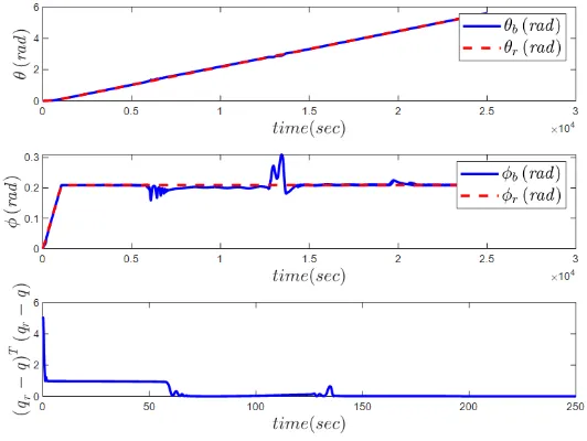
The results obtained from the nonlinear fuzzy adaptive SMC for the car-like robot have been presented in Figure 7 and 8. In Figure 7, which shows the trajectory of the car-like robot achieved by considering the effects of uncertainty and external disturbance, the robustness of the designed controller against these disturbing factors has been well demonstrated. In addition to disturbance, the effect of uncertainty has been incorporated by changing the robot body mass (increasing the body mass by 30%at time t = 60s and reducing it by 20% at time t = 130s). Figure 7 and 8 indicate that the designed nonlinear fuzzy adaptive SMC has been quite effective in dealing with the external disturbances.
Figure 8: The diagrams of vehicle angle and error norm versus time obtained by considering the effects of uncertainty, external disturbance and control signal saturation and by using the nonlinear fuzzy adaptive SMC for the car-like robot.
conditions quite successfully. This can be confirmed by the reduction of error norm and MSE values shown in the simulation results of Figures 7 and 8. Besides the satisfactory performance of the nonlinear fuzzy adaptive SMC (according to Figures 7 and 8), by comparing Figure 6 (the IANC) with Figure 8 (the nonlinear fuzzy adaptive SMC), it can be realized that in the presence of external disturbances and with the fluctuations of car-like robot mass, the nonlinear fuzzy adaptive SMC performs better than the IANC. As Figures 7 and 8 indicate, despite the presence of disturbance and uncertainty, the car-like robot has succeeded in tracking the considered path.
6. Conclusion
The necessity of using intelligent and autonomous vehicles and also the difficulty of determining the exact model of a car-like robot as well as the existence of unknown external disturbances prompted us to employ the adaptive method to deal with these problematic factors related to the automatic control of such vehicles. In this paper, two adaptive methods were devised for the control of a car-like robot. The first approach is based on the neural network (NN) with radial basis functions, which acts as an indirect adaptive neural controller (IANC). The second approach is a nonlinear adaptive fuzzy sliding mode control technique. First, a simple model was presented for the car-like robot. Then a controller was designed for the trajectory tracking control of the robot. The first controller comprises a kinematic controller with constant gains; which has been designed by defining a Lyapunov function for it. This controller also includes an IANC whose parameters are updated online. The constant parameters of the controller and also the initial values of the NN used in this controller were determined by means of genetic algorithm (GA). The nonlinear fuzzy adaptive sliding mode controller (SMC) comprises a sliding mode section, whose stability has been evaluated by defining a Lyapunov function. It also includes a fuzzy section which has been designed, for the purpose of reducing the effect of chattering, by adaptively tuning the sign function gains. The constant control parameters of this controller were also determined by means of GA. Finally, simulations were performed by considering factors such as external disturbance and model uncertainty. In the Results section, the Proportional-Integral-Derivative controller based on GA was compared with the designed IANC; which showed the superiority of the latter to the former. In addition, the IANC (the first controller) was compared with the nonlinear fuzzy adaptive SMC (the second controller). The findings indicated the better performance of the nonlinear fuzzy adaptive SMC. The simulation results at the end of this work have been presented by considering the effects of model uncertainty and external disturbance. These results reveal that the designed methods (both the first and the second controllers) can effectively deal with disturbing factors and successfully control a car-like robot in autonomously tracking a desired path.
References
[1] L.D. Burns, A vision of our transport future, Nature, 497 (2013) 181-182.
[2] If autonomous vehicles rule the world: from horseless to driverless, (Economist2015).
[3] S.A. Cohen, D. Hopkins, Autonomous vehicles and the future of urban tourism, Annals of Tourism Research, 74 (2019) 33-42.
[4] T. Litman, Autonomous vehicle implementation predictions, Victoria Transport Policy Institute (2015).
[5] C. Gkartzonikas, K. Gkritza, What have we learned? A review of stated preference and choice studies on autonomous vehicles, Transportation Research Part C: Emerging Technologies, 98 (2019) 323-337.
[6] World Health Organization (2015), ”The top 10 causes of death,” 2016. [Online]. Available: http://www.who.int/en/news-room/factsheets/detail/the-top-10-causes-of-death. [Accessed November 2018]. [7] P. Thomas, A. Morris, R. Talbot and H. Fagerlind, ”Identifying the causes of road crashes in Europe,” in Annals
[8] R. Fierro , F.L. Lewis, Control of a nonholonomic mobile robot: backstepping kinematics into dynamics, 34th IEEE Conference on Decision and Control pp. 3805-3810, 1995.
[9] J. Funke, M. Brown, S.M. Erlien, J.C. Gerdes, Collision Avoidance and Stabilization for Autonomous Vehicles in Emergency Scenarios, IEEE Transactions on Control Systems Technology, 25 (2017) 1204-1216.
[10] B.S. Park, S.J. Yoo, J.B. Park, Y.H. Choi, A simple adaptive control approach for trajectory tracking of electrically driven nonholonomic mobile robots, IEEE Trans. Control Syst, 18 (2010) 1199-1206.
[11] D. Chwa, Tracking control of differential-drive wheeled mobile robots using a backstepping-like feedback lineariza-tion, IEEE Trans. Syst. Ma Cyber, 40 (2010) 1285-1295.
[12] R. Murray, Z. Li, S. Sastry, A Mathematical Introduction to Robotic Manipulation (CRC Press, Boca Raton, 1994).
[13] ”Generic 4-Wheeled Vehicle with Independent Suspension,” Maplesoft, [On-line].Available:https://www.maplesoft.com/products/maplesim/mod elgallery/detail.aspx?id=60.
[14] F. Pourboghrat, M.P. Karlsson, Adaptive control of dynamic mobile robots with nonholonomic constraints, Computers & Electrical Engineering, 28 (2002) 241-253.
[15] G. Klancar, A. Zdesar, S. Blazic, I. Skrjanc, Wheeled Mobile Robotics: From Fundamentals Towards Autonomous Systems (Elsevier Science, 2017).
[16] J. Liu, Radial Basis Function (RBF) Neural Network Control for Mechanical Systems: Design, Analysis and Matlab Simulation (Springer, 2013).
[17] O. Mohareri, R. Dhaouadi, A.B. Rad, Indirect adaptive tracking control of a nonholonomic mobile robot via neural networks, Neurocomputing, 88 (2012) 54-66.
[18] J.-J.E. Slotine, W. Li, Applied Nonlinear Control (Prentice-Hall, Englewood Cliffs, NJ., 1991).
[19] N. Noguchi and H. Terao, Path planning of an agricultural mobile robot by neural network and genetic algorithm, Computers and Electronics in Agriculture, 18 (1997), 187-204.