Single end low voltage arcing fault location using time based formulation

Single End Low Voltage Arcing Fault Location

Using Time Based Formulation

Mohsen Mohammadi Alamuti1_{, Hassan Nouri}1_{, Mohammad Montakhab}1 _{and Alexis Polycarpou} 2

1_{University of the West of England, Bristol, UK} 2_{Frederick University, Nicosia, Cyprus}

Abstract- Due to utilizing fundamental frequency, impedance

based fault location methods to date are able to locate only permanent and linear faults. The duration of arc in low and medium voltage systems can be as short as a quarter of a cycle. This amount of time which is normal for intermittent faults is not enough for fundamental frequency based fault location algorithms. Therefore, available methods are not applicable for intermittent arcing fault location. In this paper, a novel method is proposed for arcing fault location utilizing time based formulation considering the short duration of the faults. The advantage of the proposed method over available methods is its capability for locating faults using fewer samples which is suitable for arcing faults as well as normal faults in the network. The validity of the devised algorithm is studied within the PSCAD-EMTDC environment. The produced data has been employed for the fault location algorithm and the results show a good accuracy for arcing faults.

Index Terms-- Arcing fault location, Single end, Distribution

feeder.

I.INTRODUCTION

Although today different methods have been devised in low or medium voltage networks for arcing fault detection [1-4], the arcing fault location is still a challenge for engineers. The fault location procedure is possible only after an intermittent fault turns to a persistent fault. The problem arises when this change doesn’t happen even after a couple of minutes. Dispatching repair crews to the fault area will fail to find the fault point due to no fault observation after replacement of the fuse. Sometimes it may take hours or even a couple of days until the fault re-occurs at the previous location. Travelling wave methods as well as impedance based algorithms can be utilized for arcing fault location.

A significant work has been done to address this challenge utilizing the travelling wave methods in [5, 6]. However still many problems need to be resolved for accurately locating of the fault point. Gale et all [5, 6] have introduced an online fault location equipment for low voltage underground cables. Their algorithm is based on the Time Domain Reflectometer (TDR) and Transient Recording System (TRS) method. Each of these methods has its own advantages and disadvantages. TDR is more convenient but subject to attenuation limits. Also the preferred point of connection for TDR mode is open ended. In TRS there is no need to connect units at open ends but at least two units are necessary. The main advantage is that they are not using reflected signals and only one transit along the different part of the cables is made by pulses.

Ordinary impedance based fault location methods [7-10] that are applied in medium voltage distribution systems are unable to locate arcing faults in distribution networks, due to the short duration of many arcing faults. Generally the duration of the arcing fault is less than a cycle. Also in case of persistent arcing fault, the accuracy of these methods due to neglecting the variable nature of arc resistance is not acceptable.

The raised problem due to short duration of arcing fault can be resolved via utilizing time domain algorithms. In high voltage transmission lines, time domain numerical algorithms have been used for blocking autoreclosure. A time domain numerical algorithm based on one terminal input data for blocking autoreclosure in transmission lines has been presented in [11-13]. This approach does not require the line zero sequence parameters as input data.

A numerical spectral domain algorithm devoted to arcing fault recognition and fault distance calculation has been introduced in [14-16]. Arc voltage amplitude and fault distance are calculated from the fundamental and third harmonics of the terminal voltage and current phasors. The calculated arc voltage amplitude is used to decide a fault type. Lee et. al [17] present a numerical algorithm employing synchronized phasors measured by PMU (Phasor Measurement Unit) units installed at both terminals of the transmission lines, for fault location calculation and arcing fault recognition. The proposed algorithm utilized the synchronized phasors measurement for estimating the arc voltage amplitude. From the calculated arc voltage amplitude, a decision can be made whether the fault is permanent or transient.

this method is dependant on the existence of the decay DC after the fault.

Although, time based fault location algorithms have been introduced for high voltage transmission lines for arc recognition and autoreclosure blocking, this concept can be used to generate a new algorithm for arcing fault location in distribution systems. Low Voltage fault location presents severe technical challenges and available fault location methods cannot be applied for detecting and locating all types of fault in LV systems. The difficulty is further pronounced in low voltage feeders because of private customers as end users and hence the availability of one terminal for signal measurement. At the same time, incentives imposed by the Regulator have increased the urgency to restore supplies after permanent faults and to avoid outages by reducing the incidence of repetitive intermittent faults.

In this paper attempts are made, to devise a novel single end impedance based fault location algorithm for low voltage systems which is based on the time domain formulations. This algorithm provides more accurate results as short time nature of arc is considered here whereas in the available methods arc fault is considered as a permanent solid fault instead of intermittent fault. In addition the algorithm is independent of load value which is varying hourly especially in low voltage networks.

II.INTERMITTENT FAULT CONCEPT

The voltage stress in the dielectric of LV cables is very low and hence the insulation thickness is determined by mechanical factors rather than electrical considerations. This results in high levels of instability in LV cable fault waveforms which are major causes of Power Quality problems. Hence, intermittent faults occur more often in low voltage systems rather than higher voltage systems. In terms of duration arcing faults can be divided into intermittent and persistent fault categories.

A. Intermittent faults

Intermittent faults usually occur in cables. These faults contain a conducting state during which current flows through the arc and a non-conducting state without any arc. Due to low voltage combined post-arc column deionization by insulation decomposition gases the duration of arcing state is short, normally between one-quarter cycle and one cycle.

However the length of non-conducting state is much more variable, anything from a few cycles to several minutes. The existence of humidity and solvent minerals intensively decreases the duration of the non-conducting state therefore increases the frequency of the re-ignition. Although, there is no clear explanation as to why arcs tend to reignite in roughly the same polarity [19, 20].

Intermittent faults are recognized by their repetitive fuse blowing characteristics. As illustrated in Figure 1 during arc ignition, when the arc current are crossing zero then it will be extinguished. Re-ignition of the arc may take place a few

cycles later. However, the re-ignition time may be elongated to a couple of hours. This will make a problem, when the repair crew is dispatched to the fault area due to customer calls. After reconnecting the fuse due to the nature of intermittent fault, the network continues to work properly. The repair crew can only find the fault when it turns to a solid and persistent fault. Therefore, they will have no other choice, except to leave the area. Later on, when this fault turns to permanent fault they have to go back to locate and then repair the fault. This is time consuming as well as being costly.

Figure 2 Equivalent circuit for fault location algorithm

0.11 0.115 0.12 0.125 0.13 0.135 0.14 -500

-400 -300 -200 -100 0 100 200 300 400 500

Time (s)

M

eas

ur

ed

V

o

lt

age

(

V

)

Pre-fault data sample

Fault data sample One cycle difference between pre-fault and fault samples

Figure 3 Initial guess for load estimation

0 0.02 0.04 0.06 0.08 0.1 0.12 0.14 0.16

-600 -400 -200 0 200 400 600

Time (s)

M

easu

red

Vo

lt

a

g

e

(V

)

III.FAULT LOCATION ALGORITHM

A. Fault location concept

In the proposed method, a novel time based fault location algorithm has been developed to overcome the previously mentioned problems existing in low voltage distribution systems. The proposed algorithm is utilizing the measured voltage and current from one end of the network to find the location of the arcing fault. The main characteristic of arcing fault is its short duration (around a quarter of cycle) which distinguishes arcing fault from permanent or persistent faults.

Figure 2 shows equivalent circuit employed in this paper for fault simulation. For the cable/line illustrated in Figure 2 equation (1) gives the voltage and current relationship for each phase on the assumption that an arc voltage occurs between phase A and ground:

dt di L L dt di L dt di L i R R v dt di L dt di L L dt di L i R R v i R dt di L dt di L dt di L i R v c Load c Cable cc b Cable bc a Cable ac c Load c Cable c c c Cable bc b Load b Cable bb a Cable ab b Load b Cable b b Arc Arc c Cable ac b Cable ab a Cable aa a Cable a a ) ( ) ( ) ( ) ( − − − − − − − − − − − − − − − − + + + + + = + + + + + = + + + + = (1)

where (va, vb, vc, ia, ib, ic) are measured from the low voltage side of the transformer feeder.

In single phase to ground fault (here it is assumed that phase A is involved), the faulty phase equation is used for fault location. Reformatting equation of phase A will lead to the equation below:

Arc Arc c Cable ac b Cable ab a Cable aa a Cable a

a R i

dt di L dt di L dt di L i R x

v ⎟+

⎠ ⎞ ⎜ ⎝ ⎛ _{+ + +} = − − − −

where Ra-Cable, Laa-Cable, Lab-Cable, Lac-Cable respectively shows the resistance, self and mutual impedance of the whole cable/line. In the above equation, x represents the percentage of the cable/line length and both x and arc resistance in the equation are unknown. For solving the certain number of unknowns, it is necessary to provide the same number of equations. Bearing in mind that each sample can provide us with one equation, thus with at least the same number of samples (as unknowns) one will be able to solve the equations for unknowns. Here, two samples are necessary for solving the x (distance percentage) and fault resistance which is of no importance. Therefore we have:

2 2 2 2 2 2 1 1 1 1 1 1 Arc Arc c Cable ac b Cable ab a Cable aa a Cable a a Arc Arc c Cable ac b Cable ab a Cable aa a Cable a a i R dt di L dt di L dt di L i R x v i R dt di L dt di L dt di L i R x v + ⎟ ⎠ ⎞ ⎜ ⎝ ⎛ _{+ + +} = + ⎟ ⎠ ⎞ ⎜ ⎝ ⎛ _{+ + +} = − − − − − − − − (2)

Line voltages and currents at one terminal are uniformly sampled with the preselected sampling frequency fs=1/T, where Ts is the sampling period. The current derivative for each sample is calculated from equation (3)

s s T t i T t i dt

di ( + )− ()

= ₍₃₎

By re-writing equation (2) the following matrix is obtained:

⎥ ⎦ ⎤ ⎢ ⎣ ⎡ ⎥ ⎥ ⎥ ⎥ ⎦ ⎤ ⎢ ⎢ ⎢ ⎢ ⎣ ⎡ ⎟ ⎠ ⎞ ⎜ ⎝ ⎛ _{+ + +} ⎟ ⎠ ⎞ ⎜ ⎝ ⎛ _{+ + +} = ⎥ ⎦ ⎤ ⎢ ⎣ ⎡ − − − − − − − − Arc Arc c Cable ac b Cable ab a Cable aa a Cable a Arc c Cable ac b Cable ab a Cable aa a Cable a a a R x i dt di L dt di L dt di L i R i dt di L dt di L dt di L i R v v 2 2 2 2 2 1 1 1 1 1 2 1 (4)

where [va, ia, dia/dt, dib/dt, dic/dt] are the time dependent coefficients taken from current and voltage waveforms and [Ra-Cable, Lab-Cable, Lac-Cable, Laa-Cable] is the vector of constant circuit parameters. Solving the above matrix will give both unknowns. Multiplying the calculated x by 100 will give us the fault distance in meter.

B. Load current estimation

For less than 10% of the customers, protective devices like fuses are located outside the building or factory. Therefore, the load can be easily disconnected from the network by the

dispatched crew. Disconnecting the loads causes the fault current value to become equal to the measured sending end current. However, in the majority of the sites, loads cannot be disconnected due to limited access to the private customers as end users. As a consequence, the measured current at the sending end equals to the sum of fault and load current whereas the load current is unknown. This will produce an error in the estimated fault location. This error depending on the network parameters and load values can be more than %10. Hence, for developing a precise fault location algorithm, accurate estimation of load values is very important. This is achieved through an iterative method using the pre-fault data as an initial guess.

In the first iteration the difference of the post-fault measured current and pre-fault measured current is used as an initial guess for fault current. However, in time based method the subtraction post and pre-fault data should be calculated from the corresponding samples of different cycles. This has been well illustrated in Figure 3. Due to the variation of the load current during the fault the initial guess should be updated through iterative method. In every iteration, the fault current is updated according to the following method.

After calculating fault distance x by solving equation (4), the fault voltage can be calculated from the equation below:

⎟ ⎠ ⎞ ⎜

⎝

⎛ _{+ + +}

−

= − − − −

dt di L dt di L dt di L i R x v

v c

Cable ac b Cable ab a Cable aa a Cable a a

Fault (5)

By having the fault voltage from equation (5), load current can implicitly be calculated from the following equation.

⎟ ⎠ ⎞ ⎜

⎝

⎛ _{+ + +}

−

+ +

=

− − − − − − − −

− − − −

dt di L dt di L dt di L i R x l

dt di L i R v

c load Cable ac b load Cable ab a load Cable aa a load Cable a

a load Load a a load Load a Fault

)

( (6)

After obtaining load current, fault current is calculated from the equation (7).

a load a Arc i i

i = − _{− (7)}

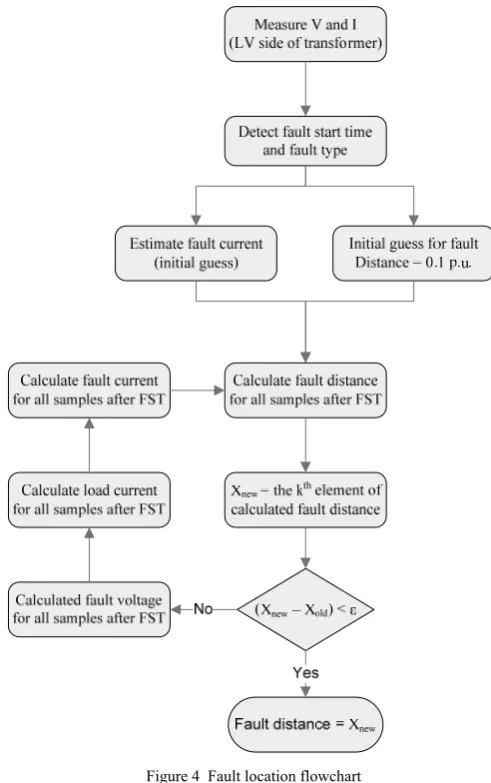
The result is used for updating the fault current in equation (2). Substituting the obtained fault current with the previous value, the same procedure can be followed until the solution is converged within the allocated error. The flowchart of the algorithm has been displayed in Figure 4. More accurate calculation of the fault current will lead to the more precise fault distance estimation.

IV.RESULT AND DISCUSSION

In order to test the proposed method a single section underground cable connected to the load was simulated within PSCAD-EMTDC environment. Figure 2 shows the network configuration. A series of 21.55 Ω resistive and 0.01162 H inductive element are composing the load in the

circuit. The cable length is 1000 meters and its impedance matrix is:

) / ( j0.503 0.66 j0.221 j0.221

j0.221 j0.503

0.66 j0.221

j0.221 j0.221

j0.503 0.66

kM

ZCable Ω

⎥ ⎥ ⎥

⎦ ⎤

⎢ ⎢ ⎢

⎣ ⎡

+ +

+ =

A. The effect of fault resistance and fault distance variation

In LV distribution, the currents are not generally monitored. In general an earth fault or higher ohmic fault will remain unnoticed, until it draws enough current to blow a fuse. If it is assumed that the lowest practical fuse for a main cable is 125 A and it is further assumed that the load current is 60% of the fuse rating, a fault will have to draw more than 50 A to blow the fuse. Therefore, a fault resistance should always be less than 6 Ω in the LV scenario. As a result in this case, the worst case scenario for arc resistance is simulated to reflect the maximum possible error. Therefore, we won’t face with higher errors produced due to the high arc resistance.

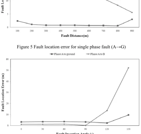
For phase A to ground faults, the calculated fault locations for various points along the cable and two different fault resistances have been displayed in Figure 5. After investigating of the figure, it doesn’t reveal any strict relationship between the estimation error and fault distance. However, the higher fault resistance leads to higher estimation error. For the proposed algorithm, the result for single phase to ground fault is reflecting the amount of error up to 20 meters for the worst case scenario.

Figure 5 Fault location error for single phase fault (A→G)

B. Fault inception angle effect

Arcing fault can appear in a random angle of a cycle. Depending on the fault environment, the arc current will be extinguished after becoming zero or another arc will ignite. Normally for the intermittent faults, arc current will be extinguished after zero crossing. Hence, duration of arc is determined by the inception angle. In other words, the bigger the inception angle, the shorter arc duration. Figure 6 shows the effect of the inception angle to the accuracy of the fault location algorithm for 3 ohms arc resistance and 500 meter fault distance. A quick glance at the figure discloses that very short arc can not provide enough data for the algorithm to locate the fault precisely. On the other hand, for faults that are longer than a quarter of cycle, arc duration doesn’t have considerable affect on the accuracy. Because intermittent faults are normally longer than a quarter of a cycle, they can be located with a good accuracy by this algorithm. The same result is obtained for negative current values (with more than 180 degree phase angle).

V.CONCLUSION

This paper has proposed a novel method for the location of arcing faults in low voltage distribution feeders utilizing single end measurements. The advantage of this method over current fault location methods is the ability of locating arcing faults which often occur, particularly in low voltage cables.

Utilizing the time based calculation, will enable the algorithm to find the location of the fault with a small number of samples. The proposed method is independent of the load value which is very important due to unpredictable and variable characteristics of the loads in low voltage systems.

For verification of the proposed algorithm, a low voltage feeder has been simulated within the PSCAD environment and the produced data has been analyzed via the algorithm. This algorithm provides accurate results as the short duration nature of arc is considered here whereas in the available methods, fault duration is assumed to be continued for at least one cycle. Obtaining accurate fault distance estimation proves that the algorithm is capable of calculating the location of short duration faults.

REFERENCES

[1] D. G. Ece and F. M. Wells, "Analysis and detection of arcing faults in low-voltage electrical power systems," presented at 7th Mediterranean Electrotechnical Conference, 1994.

[2] W. Charytoniuk, W. J. Lee, M. S. Chen, J. Cultrera, and T. Maffetone, "Arcing Fault Detection in Underground Distribution Networks— Feasibility Study," IEEE Transactions on Industry Applications, vol. 36, pp. 1756-1761, 2006.

[3] A. K. Mishra, A. Routray, and A. K. Pradhan, "Detection of Arcing in Low Voltage Distribution Systems," presented at IEEE Region 10 Colloquium and the Third International Conference on Industrial and Information Systems, Kharagpur, INDIA, 2008.

[4] B. Leprettre and Y. Rebiere, "Detection of electrical series arcs using time-frequency analysis and mathematical morphology," presented at Sixth International Symposium on Signal Processing and its Applications, , 2001.

[5] J. Livie, P. Gale, and A. Wag, "Experience with online low voltage cable fault location techniques in Scottish Power," presented at 19th international conference on electricity distribution CIRED, Vienna, 2007.

[6] J. Livie, P. Gale, and A. Wag, "The Application of on-line travelling wave fault location techniques in the location of intermittent faults on low voltage underground cables," presented at IET 9th International Conference on evelopments in Power System Protection DPSP, 2008. [7] R. H. Salim, M. Resener, André Darós Filomena, K. R. C. d. Oliveira,

and A. S. Bretas, "Extended Fault-Location Formulation for Power Distribution Systems," IEEE Transactions on Power Delivery, vol. 24, pp. 508-516, 2009.

[8] M. M. Alamuti, H. Nouri, N. Makhol, and M. Montakhab, "Developed Single End Low Voltage Fault Location Using Distributed Parameter Approach," presented at The 44th International Universities' Power Engineering Conference, 2009.

[9] X. Yang, M. S. Choi, S. J. Lee, C. W. Ten, and S. I. Lim, "Fault Location for Underground Power Cable Using Distributed Parameter Approach," IEEE Transactions on Power Systems, vol. 23, pp. 1809 - 1816, 2008.

[10] J. Mora-Flòrez, J. Meléndez, and G. Carrillo-Caicedo, "Comparison of impedance based fault location methods for power distribution systems," Electrical Power Systems Research, vol. 78, pp. 657-666, 2008.

[11] Z. M. Radojevic´, V. V. Terzija, and M. B. Djuric, "Numerical algorithm for blocking autoreclosure during permanent faults on overhead lines," Electric Power Systems Research, vol. 46, pp. 51-58, 1998.

[12] V. V. Terzija, Z. M. RadojeviC, and H. J. Koglin, "Novel Numerical Algorithm for Overhead Lines Protection and Adaptive Autoreclosure", presented at Seventh International Conference on (IEE) Developments in Power System Protection, 2001.

[13] V. V. Terzija and Z. M. Radojevic´, "Numerical Algorithm for Adaptive Autoreclosure and Protection of Medium-Voltage Overhead Lines," IEEE Transactions on Power Delivery, vol. 19, pp. 554-559, 2004.

[14] Z. M. Radojević, C. J. Lee, J. R. Shin, and J. B. Park, "Numerical Algorithm for Fault Distance Calculation and Blocking Unsuccessful Reclosing onto Permanent Faults," presented at IEEE Power Engineering Society General Meeting, 2005.

[15] Z. M. Radojevic and J.-R. Shin, "New One Terminal Digital Algorithm for Adaptive Reclosing and Fault Distance Calculation on Transmission Lines," IEEE Transactions on Power Delivery, vol. 21, 2006.

[16] Z. M. Radojevic and V. V. Terzija, "Fault Distance Calculation and Arcing Faults Detection on Overhead Lines Using Single End Data," presented at IET 9th International Conference on Developments in Power System Protection, DPSP 2008. , 2008.

[17] C. J. Lee, J. B. Park, J. R. Shin, and Z. M. Radojevié, "A New Two-Terminal Numerical Algorithm for Fault Location, Distance Protection, and Arcing Fault Recognition," IEEE Transactions on Power Systems, vol. 21, pp. 1460-1462, 2006.

[18] J. Suonan and J. Qi, "An accurate fault location algorithm for transmission line based on R–L model parameter identification," Electric Power Systems Research, vol. 76, pp. 17–24, 2005.

[19] A. Hamel, A. Gaudreau, and M. Côté, "Intermittent Arcing Fault on Underground Low-Voltage Cables," IEEE Transactions on Power Delivery, vol. 19, pp. 1862-1868, 2004.