Classification of two parameter bifurcations

warwick.ac.uk/lib-publications

A Thesis Submitted for the Degree of PhD at the University of Warwick

Permanent WRAP URL:

http://wrap.warwick.ac.uk/108587

Copyright and reuse:

This thesis is made available online and is protected by original copyright.

Please scroll down to view the document itself.

Please refer to the repository record for this item for information to help you to cite it.

Our policy information is available from the repository home page.

C lassification

of

two-parameter bifurcations

by

Martin Peters

Thesis submitted for the degree of Doctor of Philosophy

Mathematics Institute University of Warwick

T H E B R IT IS H L IBR AR Y

B R I T I S H T H E S E S

N O T I C E

The quality of this reproduction is heavily dependent upon the quality of the original thesis submitted for microfilming. Every effort has been made to ensure the highest quality of reproduction possible. If pages are missing, contact the university which granted the degree. Some pages may have indistinct print, especially if the original pages were poorly produced o r if the university sent us an inferior copy. Previously copyrighted materials (journal articles, published texts, etc.) are not filmed.

Reproduction of this thesis, other than as permitted under the United Kingdom Copyright Designs and Patents A ct 1988, o r under specific agreement with the copyright holder, is prohibited.

T H IS TH ESIS H A S B E E N M IC R O F IL M E D E X A C T L Y A S R E C E IV E D

T H E B R I T I S H r I^IB R A R Y D O C U M E N T SUPPLY C E N T R E

Boston Spa, W etherby W e st Yorkshire, LS23 7 B Q

SUMMARY

This thesis contains the classification of two-parameter bifurcations up to codimension three, using a two-parameter version of parametrised contact equivalence.

Part one contains the classification up to codimension one. The result consists of the following components:

1. A list of normal forms for the germs having codimension less or equal to one.

2. Recognition conditions for each normal form in the list, i. e. conditions that characterise the equivalence class of the normal form. These conditions are equations and inequalities for the Taylor coefficients of the germs.

3. Universal unfoldings for each normal form.

The result is obtained by investigating the structure of the orbits, which are induced by the action of the group of equivalences on the space of all bifurcation problems. Techniques from algebra, algebraic geometry and singularity theory are applied.

in

PREFACE

This thesis is divided into two parts. Each part contains its own introduction and list of references.

CONTENTS

Chapter I

Introduction

Chapter II

1. Notation 4

2. Parametrised contact equivalence 6

3. Tangent spaces 15

4. Finite determinacy 23

5. Orbits of unipotent subgroups of equivalences 26

Chapter III

1. Higher-order terms 27

2. Determining the U-orbits 31

3. Solving the B-recognition problem 35 4. Solving the E-recognition problem 44

5. Data for E-equivalence 57

6. The classification theorem 65

Chapter IV

Immer wenn uns

Die Antwort auf eine Frage gefunden schien Löste einer von uns an der Wand die Schnur der alten Aufgerollten chinesischen Leinwand, so daß sie herabfiel und Sichtbar wurde der Mann auf der Bank, der

So sehr zweifelte.

C H A PT E R

Introduction

Golubitsky and Schaeffer [6] used methods from singularity theory to study bifurcations. This involves defining an appropriate equivalence relation on the set of all bifurcation problems and classifying these up to some codimension. In [7], for example, the same authors classify one-parameter bifurcations up to codimension four using the notion of parametrised contact equivalence. This result was extended, for problems in one state variable, up to codimension seven by Keyfitz [9]. There is a multitude of other classifications — many for equivariant bifurcations.

The problem treated in this thesis is the classification of two-parameter bifurcations in one state variable up to codimension one, using a two-parameter version of parametrised contact equivalence. The result consists of the following components:

1. A list of normal forms for the germs having codimension less or equal to one.

2. Recognition conditions for each normal form in the list, i. e. conditions that characterise the equivalence class of the normal form. These conditions are equations and inequalities for the Taylor coefficients of the germs.

3. Universal unfoldings for each normal form.

In this context there is a result due to Izumiya [8], who considered germs of the form

X2+![>(».,, \ 2) . (1.1)

2

to codimension five. As we shall show even at codimension zero there are germs which are not of the form (1.1), e. g.

x3 + xA.j + Xj .

Izumiya does not give any recognition conditions.

The following is an outline of the contents of this thesis.

In chapter II we set up the theoretical basis for the methods used to obtain the classification: First we generalise the definition of parametrised contact equivalence to two-parameter bifurcations. The set of all such equivalences forms a group which acts on the space of all bifurcation problems. The equivalence classes are the orbits under this group action. For the classification it is necessary to characterise these orbits.

The first step is to show that for many germs this problem can be reduced to studying the action of an algebraic group on a finite dimensional vector space. In order to achieve this the concept of finite determinacy is used. A germ is called finitely determined if its equivalence class depends only on a finite number of its Taylor coefficients. Proving finite determinacy for a germ is more complicated than in the one-parameter case — the Malgrange-Mather Preparation Theorem has to be used.

To calculate the higher-order terms with respect to the unipotent equivalences, we use results developed for the one-parameter case by Melbourne [11]. According to one of his theorems, determining the higher-order terms is straightforward provided the equations defining the orbit are linear. Germs which satisfy this condition are called linearly determined. In the one-parameter case most germs of low codimension are linearly determined. This, however, is no longer true in the two-parameter case. Consequently, the calculations to determine the orbit become rather complicated. In this way the orbits of the normal forms are calculated with respect to the group of unipotent equivalences.

According to the decomposition of the group of equivalences the next step is to take scaling transformations into account. This is straightforward. Then the resulting recognition conditions have to be transformed into conditions with respect to the full group of equivalences. For several normal forms this turns out to be a non-trivial procedure. It involves finding certain polynomials which are invariant under the transformation. This is carried out in chapter III, section 4.

Knowing the list of recognition conditions immediately yields the classification. This is stated as theorem III. 6. 1.

Calculating the higher-order terms as described above involves selecting a particular normal form to start with. This leads to the question of how to reduce the amount of calculations by choosing the normal form in an appropriate way. We address this problem in chapter IV.

Chapter V contains a list o f diagrams giving a geometrical description of the normal forms in the classification and their universal unfoldings.

C H A PT ER II

1. Notation

We denote coordinates in IR x IR2 by x, X /, A2 • Putting A := (Xj, A 2) we define

Ex k to be the ring of all C°°- function germs IR x IR2 —♦ IR at (0, 0) e IR x IR2 .

Mx£ denotes the maximal ideal in Ex ^ .

Analogously defined are the rings Ex and Ek and their maximal ideals M x and

M Sometimes we abbreviate >M,x>x to M.

Let V be a vector space over the field of real numbers and let v j... vk e V . Then

IR { v j , . . vk } denotes the linear span of v j , . . vk .

Let G be a Lie group. We denote its Lie algebra by LG.

IR*0 denotes the multiplicative group of positive real numbers.

The function sg: IR—*IR is defined by

(

For small values of a , P and y we write hx, hxx, *lxX1Xi etc- instead- It will always be clear from the context, whether h = 0 means h(0) = 0 .

2. Param etrised contact equivalence

In this section we define parametrised contact equivalence for two-parameter bifurcations. This definition is analogous to the one introduced by Golubitsky and Schaeffer in the one-parameter case (See [6] and [7]. ). For later use two slightly modified versions of this equivalence relation are introduced. Each equivalence relation corresponds to a group and w e state some results dealing with relations between these.

To avoid repetition the following definition incorporates all the three different equivalence relations. For notational convenience we use the term E-equivalence for parametrised contact equivalence. Compare [1], [4], [5] and [10] for the concept of ordinary contact equivalence.

2.1 Definition. Two germs f , g e Mx ^ are called E-equivalent, if there exist smooth germs S, X: IR3, 0 —>lR, and A2: IR2. 0 —+IRsuch that

g(x, X j, X2) * S(x, Xj, X2) f(X (x, Xf, X2), Aj(X], X2), A 2(Xj, X2))

and the following conditions are satisfied:

X ( 0, 0 , 0 ) - 0 A j(0 . 0 ) - 0

A ^ O .O J-O (2.1)

7

<A h t (A i h 2 t o <A2>X, <A2>X2

(2.2)

Furthermore, i f the germs X, Aj, A2 and S satisfy the conditions (2.1) and additionally

f and g are called O-equivalent.

Let E be the set of all quadruples (S, X, Aj, A2) satisfying the conditions (2.1) and (2.2). E acts on Mx^ in the following way: Let f e Mx ^ and e = (S, R) e E, where R = (X, Aj, A2). The conditions in the previous definition imply that R is a diffeomorphism germ IR3, 0 —► IR3, 0. Then the action is defined by

S(0)- 1 Xx(0) - 1 (* i)x ,- 1

(*2>Xt - 0 (*2>X2 - 1

(2.3)

f and g are called U-equivalent. ShouldX, A j, A 2 andS satisfy (2.1), (23) and

(*i)x

2

e . f S ( f o R ) . (2.5)

c 2 • C1 : = ( ^ 2 ‘ S , o R 2, Rjo R 2)

With this definition of multiplication formula (2.5) defines a group action of E on The orbits generated by this action are precisely the equivalence classes corresponding to E-equivalence.

Let U (respectively U) be the set of all quadruples (S, X, Aj, A2) satisfying conditions (2.1) and (2.3) (respectively (2.1), (2.3) and (2.4)). Then the multiplication on E induces one on U and U each. In this way U and U become subgroups of E. Again, the orbits generated by the actions of U and 0 on x correspond to the U- and In­ equivalence classes, respectively.

To illustrate the difference between these various equivalence relations, we consider the linear part of an element e = (S, X, Aj, A2) 6 E, where

X fx.X j.X ^ - p x + qXj + rX2 + . . . Aj(A.j,X2) “ s Xj + t X2 + . . . A2(Xj,X2)* uXj + v^2 + . . . ;

S(x,Xj,X2) - A + B x + CXj + DX2 + . . . and p, A > 0 .

If e is in U, the linear part reduces accordingly:

X(x, Xj, X2) ■ x + qXj + rX2 + . . . Aj(Xj,X 2)“ Xj + t X2 + . . . A2(Xj, X2) ■ X2 + . . . ;

S(x,Xj,X2) =1 + Bx + CXj + DX2 + . . . •

9

X(x, Xj, X2) ■ x + () Xj + r X2 + • • • Aj(Xi,X2) = Xj + . . . A2(Xj, X2) “ X2 + • • • ;

S(x, Xj, X2) “ 1 + B x + C X] + D X.2 + . . . .

In the two latter cases the linear parts of S (i. e. S(0) ) and R = (X, Aj, A2) are unipotent matrices. The groups of diffeomorphisms induced by U and U on are also unipotent. Therefore the theory for unipotent groups (see [7a]) of diffeomorphisms developed by Bruce, du Plessis and Wall (See [3].) applies to U and U. One of their results will be stated in section 5.

In the remainder o f this section we describe some properties of the groups of equivalences defined above. The first property is a decomposition of E. We introduce some notation: Let T, the group of scaling transformations, denote the subgroup of E consisting of all equivalences of the form

X(x,X1,X2) - v x Ai(Xj,X2)* mXj A2(Xj,X2 )" nX 2 ;

S(x,X1,X2) - )x,

where n, v > 0 and m, n 0 . Let W denote the subgroup consisting of the identity and the equivalence given by

X(x, Xj, X2) - x AjfXj, X2) ■ X2

A2(Xj,X 2)« Xj ;

10

which interchanges Xj and X2 • Let N denote the subgroup consisting o f all equivalences of the form

X(x, Xj, X2) - x Aj(Xj,X2)= X1 + ŒX2

A2(Xi,X2)= X2 ;

S(x,Xi.X2) - l .

where a e IR. Furthermore, let B = T U .

2.2 Proposition. The group E can be decomposed as

E = N W B = N W T U .

this result is the following:

2.3 Proposition. GL(2, IR) can be decomposed as

GL(2, P ) = B* W* N* .

More precisely,

••(“ I

(2.6)

A proof can be found in [2], for example. Note that the order of the factors in the decomposition is not the standard one but has been reversed.

Proof of proposition 2.2: Let e = (S. X, Aj, A2). where

X(x, Xj, A.2) - p x + qX j + rX-2 + Qi(x, A|(A.i,X2>* sXj + tA.2 + Q2(Xi,X2>

A2( Xj, X2) “ u Xj + v X2 + Q3(Xi, X2);

2 2

Ql g ^ and Q2, Q3 g .

12

Xix.Xj.Xj) = x A , ( W

-= ^2 ;

S(x, Xj, X2) = 1 .

w by

X(x, Xj, X2) ■ x Ai(Xj,X 2 )“ X2

A2(Xj,X 2)“ Xj ;

S(x, X,. X2) - 1 .

and b = (S, 2£. Aj, A2), where

X (x.X 1.X2) . p x + ( r - ^ - q j X, + q X j + +

A|(X,.X2) - — + s X 2 + Q ^ - - * - i + * 2 ’)-|j

AjCXj.Xj) - “ Xj + Q 3( - ' i X r f X2.X,) ;

3(x,X1.XJ) - s ( * . “ X, + X2.X 1j .

13

2.4 Remark. E is the disjoint union of B and the set

| ( S ,X , A,, A j)6 E l (A2)i] t 0) .

and the elements of the latter set can be decomposed as described in the preceding proof.

The next statement is a decomposition of U.

2.5 Proposition. The group U can be decomposed as

u = nO .

Proof: Write u = (S, X, Aj, A2), where

X(x, Xj, X2) " x + Q X| + r X.2 + Qj(x, Xj, X,2) Aj(Xj,X2)= Xj + tX2 + Q2$-i.^2) A2(X|,X2)= X2 + Q 3^1’ ^2)«

2 2

Qi e R x ^ and Q2> Then u = n u , where n is given by

X(x.X|.X2> - x Aj(Xi,X2 )" Xi + tX2 A2(Xj,X 2 )- X2 ;

14

and u = (S. 2£. Ai> A2), where

X(x, Xj, X2) - x + q Xj + ( r - q t ) X2 + Qi(x, Xj - t X2, X2) Aj(Xj,A.2)“ Xj + Q2(Xj - 1X2, X2) A2(Xj, X2) ■ X2 + Q3$>1 " * ^2» ^2);

S(x.Xi.X2) - S ( x . X i - t X 2.X2) o

2.6 Proposition. 0 is a normal subgroup ofE.

Proof: The reasoning is analogous to the one given by Melbourne in [11] for the one- parameter case. Mapping (S, X, Aj, A2) to

S(0),xx(0), <AA ,

defines a group homomorphism from E onto IR*0 x 1R5”0 x GL(2, IR) . U is the kernel of this homomorphism and hence a normal subgroup of E.

15

3. T an g en t spaces

It is a well known feature of singularity theory that questions of equivalence can be treated on an infinitesimal level. The crucial construction involved is the tangent space to an orbit generated by the group of equivalences. The different group actions defined in section 2 give rise to different tangent spaces to the group orbits. First we give a geometrical definition of these tangent spaces. (See [4], for example.):

3.1 Definition. Let G be a subgroup o f E, LG its Lie algebra and exp: LG —* G the exponential map. Then

is called the G - tangent space o f f.

To calculate the U- and U-tangent spaces o f a given germ we use the following algebraic formulae:

3.2 Proposition.

16

T < f- U ) - t,.x { x f . X j f, X2 f, Xj fx . X2 fx , x fx ^ +

| *2 fX, ’ X1 fX, • fx2 ’*1 *2 fx2 ’ X2 fx2

₎

Proof: The results follow from definition 3.1 and the definitions of the groups U and U. □

3.3 Example. Consider f = A x 3 + B x X2 + C X j, where A, B, C ^ 0 . Then

T(f, 0 ) = «M, + < X,, X2 > + IR ^ x Xj, x X2, x Xj X2, x Xj, x Xj, Xj, Xj X2, X2

and

T(f, U) = M4 < Xj, x2 > +-V 3

f 2 2 2 2 2 \

ip ( x X^, ^ X2, x X, X2, x Xj, x X|, Xjt Xj X2, X2, X2 j .

In order to define the concept of codimension, we need another kind of tangent space.

3.4 Definition. Let f be a germ in Mx x . Then

Tt(f,E) = exJL <f,fx) + ex { fXf fx

2

17

Te(f, E) is the infinitesimal construction associated to unfoldings of the germ f. We omit the details, since they are analogous to the one-parameter case (See [7].1).

Note that all these tangent spaces are E^-modules, but — in general — not £ x x.- modules.

3.5 Definition. Let f be a germ in Mx^ . The codimension o f f denoted by cod f is the codimension of T ^f, E) as a vector subspace o f

Note that the codimension of f is finite if and only if either T(f, U) or T(f, U) has finite codimension. This follows from

The first step to determine the codimension of a germ is to show that this codimension is finite. We deal with this matter in the next section. For both germs appearing in the next example, we already assume that they have finite codimension. Consequently, we can do all calculations modulo for some k e W and this is to be assumed in this example.

T (f. E) - T(f.U) + (r{ f. f„. , f,. fv X, fv Xj fv fv X, fv Xj }

and

18

3 2

3.6 Example. 1. Consider f = x + xX j + X2 . After some calculations it turns out that

Te<r,E) = X 2 + + IR-( 1 }

and hence

Te(f.E) ’ ■

Therefore cod f = 1 .

2. Consider f = x4 + x Xj + ^ . Then

Tff,E ) = e , A { x 4 + x X , + X j.4x3 + X , j + Ex < x , l >

- Ex a{ - 3x4 + X 2 ' 4 , ‘3 + X1} + El < ’U > •

Define a homomorphism <p: Ex.X —► £x by

<p(x) = x tp ^ ) = - 4 x3 <p^) = 3 x4

19

tIjq / » •

B <p(T(f,E))

This follows from the fact that

ker (p = | - 3 X + \ , 4 x + ^ i ^ »

which ensures that <p induces an isomorphism between £Xia/Tc(f,E) and

t_x

<|{T/.E>)

The following equality holds:

^T (F.E))

-4x ,3x

<p(T(f,E))

1 {*2} .

20

The next example shows that the germ f = x4 + x2 Xj + x X2 has infinite codimension. We treat a more general case.

4 2

3.7 Example. Consider f = x + x (p&j, Aj) + x V&j, Aj) , where y e .M,^ . Then f has infinite codimension. We show this in the following way:

This expression can be estimated algebraically:

T e(f. E) c l { x4, x2 oO.), x y(X), x3. x <p(X). }

. . / 2d9(X) .. 9y(X) I j W X ) _ 3\|/(X) ^

d \, • * d \ , ■ SXj ■ ~ S ^ ~ J

c Ex,X < * - V 0 .) > .

Let I denote the ideal ^ { x, \jr(X) } . Suppose now that f has finite codimension. Then

K k c T e(C E) c I

21

V(I) c V

This, however, is impossible, since the dimension of V(I) is 1. Hence f has infinite codimension.

For use in the next section we introduce a name for a subspace of Te(f, E) which is an Ex>X*niodule.

3.8 Definition. Let f be a germ in M Xtx- Then

R T , ( f , E ) = e xJL { f , f x }

is called the restricted extended E-tangent space off .

The following result will be needed later:

3.9 Proposition. Let f be a germ in Mx x and g e E. Then

T(g 0 ) - g . T(f, 0 ) .

22

- | ^ ( * ' (*J exP<‘ A)«).f) J

J

’ e ' | l i ( i * ' «po A) e ) • f ) oIa e lCj| . <3 1 >

Since U is normal in E (See proposition II. 2. 6. ) , g 1 0 g = 0 holds for all g e E. Therefore the curves g‘‘ exp(t A) g in U range over all curves in 0 through the identity element in U. This implies that the expression in (3.1) is equal to

g ■ | expd A ) . f ^ J A - E L O j

= g • T(f, 0 ) ,

23

4. Finite determinacy

Due to the mixed module structure of Tc(f, E), proving finite-determinacy for two- parameter bifurcations is rather complicated. In the one-parameter case this problem can be circumvented: There it is sufficient to consider RTc(f, E), since this space has finite codimension if and only if Te(f, E) has. (This result, which is due to Damon, is stated in [7]). This is no longer true in the two-parameter case.

It is a theorem of Damon (theorem 10.2 in [3a]) that a germ f is finitely determined, if and only if it has finite codimension.

In the remainder of this section we abbreviate T e(f, E) and RTe(f, E) to Te(f) and RTc(f) respectively.

The following method will be used: For some appropriate pairs (k, £) o f non-negative integers the property

is verified. Here Te(f) and \ are regarded as ¡^-modules. Instead of checking (4.1), we shall use the statement in proposition 4.2 below. First, though, it is necessary to introduce some more standard terminology from singularity theory, see m . [4], [5] and [10].

4.1 Definition. A germ f 0 e Ex has finite K-codimension, if

(4.1)

TJC(V

<V}

24

4.2 Proposition. Let f e and fo :=f(x, 0, 0) . Iffo is o f finite K-codimension then the condition

implies that

c T'<f> ■

Proof: The statement is an immediate consequence of Nakayama’s lemma, once it has been shown that £x^ /R T e(f) is a finitely-generated £x-module. We show this in the following way: Since fg has finite K-codimension, there exist germs m j, . . mk e t x such that

mk } .

Using the following isomorphism

TeK(f„) RTc(f) + < A.,, Xj >

we obtain

25

or equivalently

^ ... ™k> + < ^ 1 ^ > ExA- <4 2 >

Since 8X ^/RTe(f) is a finitely-generated Ex x-module the following version of the Malgrange-Mather Preparation Theorem can be applied (See [10],p. 134 ):

4.3 Theorem. Let M be a finitely-generated £x x-module, nt], . . . . mk e Sx x> N on ^xXsubm odule o f M and n(x, X) := X . Then the following conditions are equivalent:

A) N + t x { m j...m k] = M

B) N + ¡R {m j...mk } + (n * M x )M = M .

Here 7t denotes the ideal generated by the components of it.

Putting M = £x x and N = RTe(f) it follows that condition (4.2) is equivalent to

cxjL „ , , ...' V

i. e. £x^/R T e(f) is a finitely-generated E^-module. □

26

5. Orbits of umpotent Subgroups or Equivalences

The following theorem of Bruce, du Plessis and Wall shows why it is useful to consider the unipotent subgroups of equivalences defined in section 2.

5.1 Theorem. Let U be an unipotent affine algebraic group over IR acting algebraically on a real affine algebraic variety V. Then the orbits o f U are closed in the Zariski topology ofV , i. e. they are real algebraic subvarieties ofV .

Proof: See [3].

5.2 Rem ark. If G is an algebraic group acting algebraically on a smooth algebraic variety, then the orbits are smooth semi-algebraic sets. See [4] for a proof of this fact. Under the assumptions of the preceding theorem and if V is smooth — in particular, if V is a finite-dimensional vector space — the orbits are smooth real algebraic subvarieties of V.

27

CHAPTER III

1. Higher - order terms

We give the definition of higher-order terms and some results due to Melbourne (see [11]), who proved them for one-parameter bifurcations.

1.1 Definition. Let fb e a germ in M x ^- Then

M(f, V) :« f p e MXtX / f + p e U . f )

= { u . f ■ f / u e U ) .

Note that M(f, U) consists exactly of those germs that do not change the equivalence class of f when added to it. Hence determining M(f, U) solves the recognition problem. However, to do this in practice, we need a slightly different concept of higher-order terms. In order to define this we introduce some terminology first.

1.2 Definition. Let G be a subgroup o f E. A subspace V o f M ^ i s called G -intrinsic, if it is invariant under the action o fG .i.e . G .V c V . I f a subset M o f M X'X contains a unique maximal G-intrinsic subspace, then this is called the G-intrinsicpart ofM and is denoted by Ut qM .

1.3 Definition. Let U be a unipotent subgroup o f E. We call

28

the module o f U-higher-order terms.

1.4 Theorem. Let f be a germ in M x % o f finite codimension and U a unipotent subgroup o f E. Then

A) P(f, U) = I tr y M(f, U) ,

B) P(f,U) = ltru T(f,U) .

Proof: See [11]. The facts that U is unipotent and its action on Mx,x is linear are crucial. The proof works for the two-parameter case as well.

Part B) of the preceding theorem is useful for calculations. The first step to determine P(f, U) is to calculate T(f, U). the second is to find its U-intrinsic part. To do this we use the following criterion:

1.5 Proposition. Let M c Mx ^ b e a subspace o f finite codimension. Then M is U -intrinsic if and only if LU .M czM.

Proof: See [11].

1.6 Remark. To find intrinsic parts of subspaces it is useful to note that spaces of the form

29

where k, t e DJ0 are obviously E-intrinsic and hence G-intrinsic for any subgroup G of E.

1.7 Example. Let f = A x 3 + B x + C\ 2 * where A, B, C ^ 0 . Then

T(f,U) = M4 + « X j.X jï3 + IR | x2 X,, x2X2, x X, X2, x X.2 x *-2. Xt X2' Xl }

By remark 1.6

M + <X1,X.2 >

is U-intrinsic and hence

M + <Xr X2> c P(f,U)

holds. By applying the criterion in proposition 1.5 it follows that

P(f,U) = M4 + < \ V X2 >3 + b| x2 X2,x>.1X2,xX |xi»7 Aj} ■

For later use we define another concept related to intrinsic subspaces.

1.8 Definition. Let V be a vector subspace o f Mx x and G a subgroup o f E. Then

v ° . = X a •» ■

30

1.9 Proposition. Ve is the smallest G-intrinsic subspace containing V, i. e. it satisfies the following two conditions:

A) V c Ve and Ve is G-intrinsic.

B) If W c Mx x is a G-intrinsic subspace containing V, then Ve c W .

31

2. Determining th e U-orbits

Once P(f, U) is known, it is possible to determine the U-orbit of f, more precisely we determine

U . f P (f.u) '

This is done by explicitly performing the coordinate changes giving U-equivalent germs to f.

2.1 Example. Let f = A + B x Xj + CX2 , where A, B, C £ 0 . P(f,U)was

determined in the preceding section, example 1.7. Working modulo P(f, U) we obtain the U-orbit of f by first truncating equivalences (S, X, Aj, A2) in the following way:

X(x,Xj,X2) = x + pX1 + q X 2 A jftj.X j) “ + r *-2

2 2

A2(X,j, = X2 + sX,j + tX.jX2 +uX 2 ;

S(x,X|,X2> = 1 + a x .

Now define

h(x, Xj, X2) S(x, X j, X2) f(X(x, X j, Xj), A|(Xj, X2), A2(Xj, X2)).

32

(1 + a x) (a (x + p Xj + q Xj)3 + B (x + p Xj + q X2) (X, + r X j 2 + C ^ X2 + s X j + t X|

x

2

x

2

^

Modulo P(f, U) this reduces to

(1 + a x) ^ A (x + p Xj + q X2)3 + Bx>?1 + C ^ X 2 + s X j j j .

Expanding this yields

C sXj + 3 A p x 2 Xj + A x3 + CX2 + C ax X 2 + (b + C a s + 3 A p2 ) x X2 + terms in P(f, U)

Using this result, we obtain a parametrisation of U . f / P(f, U ) . The coordinates in this space are the Taylor coefficients of h. The parametrisation is

h =0 h = 0

X

h » 0

X X

h, « 0

hxxX, “ 6 A P

33

• C a

2B + 2 C a s + 6 A p 2 .

According to theorem II. 5. 1 U . f / P(f, U) is an algebraic variety. Eliminating the parameters p, s and a yields the equations defining it:

h - 0 hx = 0 h x x 'O \ - o h x X ," 0

hxxx “ 6 A

6 A c h x l , l l " 6 A h l 1X1hxX2 * C h xxl, - 1 2 A B C .

These are the U-recognition conditions for the germ f, i. e. each germ h whose Taylor coefficients satisfy these equations is U-equivalent to f. We rewrite the equations in the following way:

h - 0 hx = 0 hxx = °

\ - 0

I'xJl, " ®

35

3. Solving the B-recognition problem

In this section we show how to obtain the B-recognition conditions of a germ, when the U-recognition conditions are already known. The following example illustrates the procedure.

3.1 Example. Let f = e x3 + 8 x X2 + X2 , where e, 8 e {-1, +1 }. Since

B = T U = U T

h e B . f holds if and only if h e U . k for some k e T . f . The T-orbit of f is

T . f = ^ e j x v 3 x3 + 8 n v m2 x X2 + n n Xj | v > 0 ;m ,n £ 0 ^ .

This expression shows that k G T . f holds, if and only if k is of the form

A x3 + B x X2 + C X2 ,

where A, B and C satisfy the following conditions:

sg A = e

sg B = 6 (3.1)

C * 0 .

36

h = 0 hx = 0

sg hxxx = e \ - 0 • v °

hx X , - °

» « „ hxxX , 0 hx x l, ^xXjXj hxX2 0

V . s

We now give a list of certain germs and the corresponding B-recognition conditions. The germs have been chosen according to the following consideration: A K-versal unfolding of the germ x m (m £ 2) is given by

m x

where (Xj...a m_i e IR (See [1], [4], [5] and [10]. ). Hence every two-parameter germ f(x, X2, Xj) is E-equivalent to some germ o f the form

* " + <P,(X,,X2)x m"2 + . . . + <l>m_2<*T*2>* + <Pm-1<5Cl- X2> '

38

e x3 + x Xj + X2

where e e { -1,+1 }

h - 0 hx =0 hx*=0 sg h Xxx = e

40

e x 2 + 5(X 2 + X^) where e, 8 e {-1, +1 }

h - 0 hx » 0

\ - o

hx2 " 0 sg hxx = e sg Dj = e 8

sg H = e ,

where

and

D.

-h.x, 1

X A1A1

h„ h.x, h.Xj

H - \ x , _{V .} ''»Xj hx,x, - x *

41

1 2 2

e x + 8 ( X ,

-where e, 8 g {-1,+1 )

h - 0 hx = 0

\ - o

sg hxx = e sgD! = e 8 sg H = - e ,

where

hxx hxX,

c i

-Nx, \ x ,

\ x , hxXj H - h*>M V i hx1x2

^X^ _{V a V a}

4. Solving the E-recognition problem

Once the B-recognition problem has been solved, there is one additional step to solve the E-recognition problem. This procedure is based on proposition II. 2. 2 and is therefore a consequence of the Bruhat decomposition for GL(2, IR). Since this decomposition is valid for GL(n, IR), the method described below can be applied to bifurcations having more than two parameters.

4.1 Proposition. Let f and h be germs in Mx Then the following statements are equivalent:

A) h e E . f .

B) Either h e B . f or there exists c e IR such that h(x, a X j + X2,&j) e B . / .

Proof: We use the decomposition of E given in proposition n. 2. 2 .

A) =► B): Let h = e . f , where e e E . According to remark II. 2. 4 and proposition II. 2. 2 either e e B or e = n w b , where n e N , w e W and b e B . In the latter case it follows that

( w"1 n'1) . h = b . f .

By the definition of the groups N and W there exists a o e R such that

( ( w'1 n'1) . h ) (x, Xj, Xj) = h(x, o Xj + Xj, Xj)

The implication B) =» A) is proved similarly. □

In order to apply part B) of the proposition it is necessary to know how the Taylor coefficients of h(x, a X1 + X2, ^l) relate to those of h. This relationship is as follows:

4.2 Proposition. Let h be a germ in and

h*(x, Xj, X ^ h(x, 0 X j + X2, Xj)

for some a e F t. Then

Proof: Fix (a ', y') e No3, choose an integer m such that m £ a ' + P' + Y and consider the m-jet of h:

This implies

o x lij Çk a.y+k.p-k o+P+Y^m

46

To obtain h we multiply by a'! P'! y i :

We now solve the E-recognition problem for three particular germs. These results are stated in theorems 4.3, 4.4 and 4.6.

2 2 2

4.3 Theorem. Let f = e x + S ( A j + X2) , where e , S e { -1, +1} and let h b ea germ in M x ^ . Then h is E-equivalent to f if and only if h satisfies the following conditions:

h = 0 (4.1)

hx = 0 ( 4 2 )

s g h „ = e ( 4 3 )

h i — 0

Al (4.4)

h i — 0

X2 ( 4 5 )

s g D j = e S (4.6)

s g H = e . (4 .7 )

47

D t

-hxx

1

\A f x

and

h„

hx l l ^A/A2

hxX2 ^*1*2 ^A2*2

Proofs both of this and the next theorem will be given following remark 4.5 .

4.4 Theorem. Let f = e x 2 + X2 - - where e e f - 1 , ^ 1 ) and let hbe a germ in ■ Then h is E-equivalent to f if and only i f h satisfies the following conditions:

h = 0 (43)

hx = 0 _{(4 9 )}

s g h „ = e (4.10)

h i = 0

*l (4.11)

hx = 0

*■2 (4.12)

sg H = - e . (4.13)

48

hxx hxX_xAt hxX2

hxX_{*A1 hx xAiA1} hxtx2

hx l2 \ * 2 _^*2*2

4.5 Remark. The determinant H appearing in theorems 4.3 and 4.4 is the determinant of the Hessian of the function h . The results show that no third-order-terms appear in the recognition conditions. That is, f is 2-determined. Therefore the classification corresponds here to the classification of quadratic forms allowing linear coordinate changes which preserve the sign of hxx . For example, taking e = 5 = 1 in theorem 4.3 the recognition conditions

hx* > 0 Dj > 0 H >0

are exactly the conditions for the quadratic form defined by the symmetric matrix

«X, hx,x, ^1^2

h* * 2 i

to be positive definite.

49

h - h h* _{" hx}

“ hxx

\ = h, + o h , *2 A1 = h.

hà , - K k t * a h xX, " h,x ,

- W 2 0 l v .

^1*2 ^1 ^ 2 + °^ 1 ^ 1 ^*2*2 hA.,A.i

Applying the B-recognition conditions to h* and substituting these expressions yields the following: (4.1), (4.2) and (4.3) are obviously preserved. (4.4) and (4.5) are transformed into

\ + c\

■ 0 ,

and these equations are equivalent to

\ - 0

50

Now consider conditions (4.6) and (4.7). Let := hxx H . By (4.3) condition (4.7) is equivalent to

The following identity holds:

where

and

hxx h,X, hxXj hX,X2

hxx hxJ4 hxX2 hX2X2

(4.14)

(4.15)

Now we determine the transforms of the three determinants D lt D* and D2 . After some calculations it turns out that Dj transforms into D2 + 2 a D* + o 2 D j, D* into D* + a D j and D2 into Dj. Now consider conditions (4.6) and (4.14). (4.14) implies

sgD , = sgD 2 ,

51

D , D2 > ( D ’)

Hence (4.6) is equivalent to sg D2 = e 8 . This transforms into sg Dj = e 8 . Hence condition (4.6) is preserved. The transform of the determinant in (4.15) is

• 2 •

D 2 + 2 o D + 0 D j D + o D j

D* + a D j D j

- D ,D 2 + 2 0 0 , 0 * + <j2 D2 - (d’) - 2 a D 1D, - o 2 D^

D1 D'

Hence 'F is invariant under the transformation and condition (4.14) is preserved as well. Since hxx is invariant under the transformation, it follows that H is invariant. This proves the result. □

Proof of theorem 4.4: According to table (3.6) the B-recognition conditions for f are (4.8) — (4.13) plus

s g D , - e . (4.16)

The invariance of (4.13) under the transformation of the Taylor coefficients follows in the same way as in the preceding proof. Using the same definition for 'F as above (4.13) is equivalent to

52

Now consider condition (4.16), which transforms into

sg(E>2 + 2 oD* + o2 D,) = e . (4.18)

Suppose that Dj ^ 0 . Then the quadratic polynomial in (4.18) has - 4 'F as its discriminant. By (4.17) this discriminant is positive. Hence the polynomial assumes negative and positive values, since it has two distinct real roots. Suppose now that Dj = 0 . By (4.17) D* does not vanish and hence the expression in (4.18) assumes positive and negative values.

We have shown that in both cases there exist values of a such that (4.18) holds without further restrictions on Dj, D* and D2 . By proposition 4.1 the result follows. □

3 2

4.6 Theorem. Let f = e x + S x + X2 , where e, S e {-1, + 1 ) and let hb ea germ in . Then h is E-equivalent to f if and only if h satisfies the following conditions:

h = 0 (4.19)

hx = 0 (4 2 0 )

ha = 0 (4 2 1 )

Sg hjoa = E (4.2 2 )

A - 0 (4 .2 3 )

r t o (4 .24 )

53

and where

and

K 1

hk_At

2 K - K2

^xxx hxxXJ 0

K 1 - hxxX, h xX,XJ hxX2

0 hX l hX_*■2

hxxx hxxX2 0

K « ^xxXj hxXtX2 hxX2

0 _hXX

K1K2

^XXX hxxX2 0

k

2

0 _hx

₂

₂

*■1

Proof: The proof is divided into two steps.

Step 1: We show that the B-recognition conditions for f given in table 3.7 are equivalent to (4.19) — (4.24) plus the condition hj^ = 0 . It is sufficient to show that

54

hxX,=0 K , * 0

are equivalent to

\ = 0 (4.25)

A « 0

r* o .

Assume the conditions stated first hold. Since hj^ = 0 , T = h ^ K j . Since h^ ^ 0 , it follows that T jt 0 . = *1xX1 implies A = 0.

To show the converse, note that again T = h ^ K] . Hence h ^ jt 0 and K ] ^ 0 . Since 0 = A = - h ^ h ^ ^ , it follows that h ^ = 0 .

Step 2: We apply conditions (4.19) — (4.24) and (4.25) to the function

h*(x, Xj. X2) h(x, o X, + X2. X,).

We express the Taylor coefficients of h* according to proposition 4.2. Apart from the formulae stated in the proof of theorem 4.3 we need

^ x x X j ■ hx x X j + ° hx x l ,

^xxA ^

^xXjXj _{■ h, » * +} 2 0 h >‘ 1>5

hxX,X2 + o l l xX1X1

h« ^ hxX,X,

55

hi, + a hi, = 0 ._{k2 A.,}

The transform of A is

\ * a\ \

hxXj + ° hxX, hxX,

(4.26)

\ \

l'xX2 hxX, + a

hxXj hxXj

- - A .

Hence (4.23) is preserved. Now consider the transform of T. After some calculation it turns out that K , transforms into K2 • 2 K* - a K , . Let Q denote the transform of 2 K* - K2 . Then T transforms into

Kj - 2 K* - o Kj Q \ + o \ \

Condition (4.26) implies that this is equal to

hXj ( K 2 - 2K* - a K ,)

- hXi( K 2 - 2 K* ) - a hX( K,

By (4.26) this is equal to

56

2 K * - K j

\

- r .

This calculation shows that T is invariant under the transformation and hence condition (4.24) is preserved. By (4.24) hXj and h* cannot both vanish. Therefore there exists a o e I R satisfying (4.26) if and only if hj^ * 0 . It is trivial to show that (4.19) — (4.22) are preserved.

We have shown that h * e B . f holds if and only if (4.19) — (4.22) hold and

\ + o

A - 0 r ^ o .

57

5. Data for E-equivalence

We now give lists of the E-recognition conditions for a collection of normal forms. These germs correspond to those in section 3, except that some of them are E- equivalent to each other like

2 2

x + Xj and x + X2 .

The reasons for choosing the germs are discussed in section 3.

Proofs for the recognition conditions in tables 5.3, 5.4 and 5.5 are given in section 4. The proofs for the other results are considerably easier. In fact, the relevant steps appear in the proofs in section 4 as well — as the rather trivial parts. For this reason these proofs are omitted here.

60

e x 2 + s a 2 + 4 ) where e, 8 g {-1,+1 }

codimension 1 unfolding term: 1

h - 0

h* * 0

s g h „ - e \ - o hx2 - 0 sg Di = e 8

sg H = e ,

where

and

D 1 ■ h«x

hx l , \ x .

hxX,

H - \ x , **X,Xi

61

*■ A^ A l

e x + - ^2

where e e {-1,+1 )

codimension 1 unfolding term: 1

h - 0 hx « 0 sg hxx = e

sg H - - e ,

where

h» i, hx.,».1

h»>l2 hJl,l2 h^2X2

62

3 _ ,2 ,

e x + 5 x A.j + ^2

where e, 8 e { -1,+1 }

codimension 1 unfolding term: x

h - 0 hx - 0 h,x = 0 sg h xxx = e

A - 0

r ^ o

where

and where

\ \

hx^l ^*^2

K , 2 K * - K j

\ \

hxxX, 0

hxXjXj hxX,

hX,X,

\

65

6. The classification theorem

In this section we give the classification o f two-parameter bifurcations up to codimension one.

6.1 Theorem. Let h be a germ in Bx Ji satisfying h = hx = 0 . Let the codimension of h be less than or equal to one. Then h is E-equivalent to one o f the following germs:

w here e . S e f - 1 , + 1 } .

e x 2 + X j

2 . 2 , 2

e x + A j - X2

e x 2 + S C X 2 + Ji2)

e x + x X j + X2

e x 3 + S x X 2 + X2

e x 4 + x X j + X 2 ,

66

67

Suppose h e Sx)l satisfies h = hx = 0 . Starting with hxx and following the arrows in the flow chart, the diagram shows how the Taylor coefficients determine the equivalence class of h.

68

CHAPTER IV

1. Efficient calculation of the higher-order terms

In this section we describe a result, which is relevant for choosing the normal forms which were used in section III. 2 to calculate the U-orbits. The following example illustrates the importance of choosing the normal form appropriately.

3 2

1.1 Example. Consider the germ f = e x + 8 x A.j + X2, where e, 6 e {-1, +1 }. f is 3 2

E-equivalent to g = e x + 8 x + X j. It is possible to solve the E-recognition problem for g instead of f. However, the calculations are a great deal more complicated for the following reason: The higher-order terms for f are given by

P(f,U) = M4 + < .

(Compare example III. 2. 1.), whereas

P(g,U) « M4 + .

Hence U . g / P(g, U) has five extra dimensions compared to U . f / P(f, U) . As a consequence the parametrisation of U . g / P(g, U) turns out to be very complicated. However, it is possible to check that it eventually results in the same E-recognition condidons as for f . 1 Clearly, it is advantageous to choose f and not g as the normal form.

69

The example shows that it would be useful to have a criterion which allows to distinguish between f and g. The result which will be given below is such a criterion, which works in many cases. It is based on the relationship between the groups U and U.

Let f be a germ in M.x x and g(x, Xj, X2) := f(x, X2> Xj) . We consider the tangent space T(f, U). Its relationship with T(f, U) is given by

Hence it is trivial to compute T(f, U) once T(f, Û) is known. It is obvious that the expression

is symmetric in the differential operators appearing with respect to exchanging Xj with X2 andd/dXj and 9/9X2. Let w e W be the equivalence interchanging Xj and X2 (See section II. 2.). Then g(x, Xj, X2) = f(x, X2, Xj) = w . f . From proposition II. 3. 9 we obtain

This means that when T(f, U) is already known, T(g, U) is obtained by exchanging Xj with X2 in T(f, U). Again it is then trivial to determine T(g, U) by adding the one­ dimensional space IR • (X2 gj^} .

}

T(g, Û) - T(w . f, Û ) «* w . T(f, Û) . O D

70

1.2 Theorem . Let f be a germ in o f finite codimension. Then the following statements are equivalent:

A) P ( f,0 ) <=P(f.U) .

B) For all p e P(f, U)

Xk2 ^ € T ( f . U ) dXj

fo r all k e DJq.

1.3 R em ark. Note that statement B) does not involve P(f, U). Hence it can be checked once P(f, 0 ) and T(f, U) are known. For this X2k 3 kp /d X 1k e T(f, U) has to be checked only for a finite number of integers k and for a finite number of germs p,

since f is finitely-determined.

Theorem 1.2 can be used in the following way: Let f and g be defined as above. The first step is to calculate T(f, 0 ) and to determine P(f, U) = Itr(; T(f, U) by theorem III. 1. 4. This immediately yields P(g, U) by exchanging Xj with X2 in P(f, U), since P(g, U) = Itr(j T(g, U) and by equality (1.1). Applying the theorem it is possible to check, whether

P(f, 0 ) c P(f, U) or P(g. 0 ) c P(g, U) (1.2)

holds. The germ which the corresponding inclusion is satisfied for will then be chosen for calculating its U-higher-order terms. For many of the germs appearing in the classification theorem in section III. 6 one of the inclusions in (1.2) is satisfied.

71

where A, B, C £ 0 . Then

T(f, U) = M + < X,, X>2 > + I R ^ ^ x ^2» * ^2* ^ ^ ^ 2 ’ ^1* ^1 ^2’ ^ 2 ^ »

P (f,0 ) = m“ + « X j . X ^ 3 + IR | x 2 X j, x X , X j,x X y X , X2, X ^ ,

In this case T(f, U) = T(f, U) a n d it turns out that condition B) o f theorem 1.2 is

satisfied. To see this it is only necessary to check

X2 ^ T e W U )

ax,

where p is one of the monomials

2 “X. X. X \ X X^

As a consequence P(f, U) c P(f, U ) . In fact, in this case P(f, U) = P(f, U ) .

For g we have

T(g, U) = M + < X,, X2 > + IR ^ x Xj, x X2, x X, X^, x X,, x X ,, X ,, X, X2, ^2^ >

P(g, 0 ) = M + < X ,,X2> + IR ^ x X ,, x X, X2, x X,, X, Xj, X, ^

and it turns out that condition B) is n o t satisfied. Hence P(g, 0 ) P(g, U ) — in fact,

72

2. Consider f = x3 + x + X2 and g = x3 + x ^ 2 + X j. For these germs neither P(f, Û) c: P(f, U) nor P(g, Û) c P(g, U) holds. The codimension o f f is two.

We now give the proof of theorem 1.2. First we state a lemma.

1.5 Lemma. Let f be a germ in o f finite codimension. Then the following statements are equivalent:

A) P(f, Û) <=P(f, U) .

B) There exists a U-intrinsic subspace V o f T(f,U) such that P(f, Û) c V .

C) For all p e P(f, Û) U . p c T(f, U) .

Proof: A) =» B): This is trivial, since P(f, U) is U-intrinsic.

B) =» C): Suppose P(f, Û ) c V c T(f, U) for a U-intrinsic vector space V. Then

U . V c V c T(f, U) ,

which implies C).

Q =» A): Condition C) implies

p* P(f.Cl)

73

Pif. Û)U c ItruTif, U) = P(f, U) .

Hencc

P(f, Û) c P(f, Û)U c P(f, U) . O

Proof of theorem 1.2: Assume P(f, U) c P(f, U) holds and let p e P(f, U) . It is sufficient to prove condition B) for the case, when p is a polynomial. To see this note that since f is finitely-determined T(f, U) can be written as

T(f, 0 ) = M + V ,

where V is a finite-dimensional vector space. Mk is obviously U-intrinsic, hence

M k c P(f, 0 ) .

Therefore we can write

P P + r ,

where r e X and p is a polynomial. It is trivial to show that X, —- is in M and hence

ax.

X j- ^ 4 € * c T(f, U)

d \ 2

for all k e W0 .

74

k -J

p(x a, + t x2,x.2) - p (x ,x ,.x 2) »

y i

X 2) i (1.3)

for some number k e N0 . Applying this formula for k pairwise distinct values t j , . . tjj and using the abbreviations

w. := pix.Xj + t-A.2,X2) ~

Pj * jl 4 j pCx. x 2.

oA.j

for i, j = 1 , . . k , we obtain the following linear system of equations:

‘1 ‘1 • • • ‘l *2 *2 • • • £

^ s. k

Since Wj e T(f, U) for i = 1, . . k and the matrix in the system is invertible, it follows that

ax',

75

To show the converse first note that it is again sufficient only to consider polynomials p e P(f, U) and an equivalence u e U . According to proposition II. 2. 5 we can write u = n u , where n e N and u € 0 . We have

u . p = (n Q) . p

= n . (0 . p) .

Since P(f, 0 ) is U-intrinsic, u . p is in P(f, U). Define p := 0 . p . Then

u.p(x, Xj.Xj) = n.jKx.Xj.Xj)

- p(x. A., + tX j.X j)

76

CHAPTER V

1. Geometrical description of two-parameter bifurcations

This section contains diagrams depicting the zero-sets and discriminants of the normal forms in the classification and their universal unfoldings. The discriminant associated to a given germ f e M.x ^ \s the following set

The coordinates in the diagrams are oriented as follows:

Coordinates for the zero-sets Fig. 1.1

*2,

*1

103

References

[1] Arnold, V. I.; Gusein-Zade, S. M.; Varchenko, A. N. : Singularities of Differentiable Maps. Vol. 1. BirkhSuser, Basel / Boston / Stuttgart: 1985.

[2] Brieskom, E .: Lineare Algebra und analytische Geometrie. Band 1. Vieweg, Braunschweig/Wiesbaden: 1983.

[3] Bruce, J. W.; du Plessis, A. A.; Wall, C. T. C .: Determinacy and unipotency.

Invent. Math. 88 (1987), 521 — 554.

[3a] Damon, J . : The unfolding and determinacy theorems for subgroups of A and K. Mem. Am. Math. Soc., 50 (306), 1984.

[4] Dimca, A. : Topics on Real and Complex Singularities. Vieweg, Braunschweig/ Wiesbaden: 1987.

[5] Gibson, C. G .: Singular Points o f smooth mappings. Pitman, London / San Francisco / Melbourne: 1979.

[6] Golubitsky, M.; Schaeffer, D. G. : A theory for imperfect bifurcation via singularity theory. Commun. Pure Appl. Math. 32 (1979), 21 — 98.

[7] Golubitsky, M.;Schaeffer, D. G. : Singularities and Groups in Bifurcation Theory. Vol. 1. Springer, Berlin / Heidelberg / New York: 1984.

[7a] Hochschild, G. P .: Basic Theory o f Algebraic Groups and Lie algebras.

Springer, Berlin / Heidelberg / New York: 1981.

[8] Izumiya, S .: Generic bifurcations of varieties. Manuscripta math. 46 (1984),

104

[9] Keyfitz, B. L. : Classification of one state variable bifurcation problems up to codimension seven. Dyn. Stab. Syst. 1 (1986), 1 — 142.

[10] Martinet, J. : Singularities o f Smooth Functions and Maps. Cambridge University Press, Cambridge: 1982.

[11] Melbourne, I. : The recognition problem for equivariant singularities.

C o n te n ts

1 Classification o f two-parameter bifurcations 107

1 In tro d u ctio n ...107 2 T he classification up to codimension 3 ... 108 2.1 The classification th e o re m ... 108 2.2 Some additional information ...114

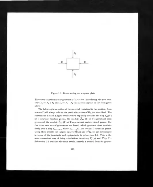
2 Equivariant bifurcations with group action on state and pa­

ram eter space 117

1 In tro d u ctio n ...117 2 General definitions and background... 118 2.1 N otation...118 2.2 Definitions and determinacy th e o r e m s ...118 2.3 An example with Z j-sy m m e try ... 122 3 D i-sy m m etry ...124 3.1 Introduction ... 124 3.2 In v a ria n ts ... 126 3.3 Equivariants ... 128 3.4 Tangent spaces for the D .|-ac tio n ... 134 3.5 The generic normal fo rm ... 138 3.6 Geometrical description of the generic normal form . . 151

C h a p te r 1

C lassificatio n o f

tw o -p a ra m e te r b ifu rcatio n s

1 I n t r o d u c t i o n

This chapter contains an extension of the work in p art one of this thesis. The result is a classification of two-parameter bifurcations in one state variable up to codimension 3.

The classification theorem is stated in subsection 2.1. The normal forms are obtained by classifying the orbits arising from the action of the group of equivalences inductively on degree using Mather’s lemma [Mat70]. The necessary determinacy results are then obtained by calculating the unipo- tent tangent spaces using results of Melbourne and Gaffney [Mel88], [Gaf86] based on work by Bruce, du Plessis and Wall [BdPW87]. A list of miniversal unfoldings of the germs in the classification theorem is also given.

Subsection 2.2 contains some examples of germs th at have codimension greater than 3.

The work contained in part one of this thesis has meanwhile appeared in summarised form in [Pet91]. The normal forms given there also arise in a completely different context as p art of another classification by Arnol’d in the paper [Arn76].

N o ta tio n in c h a p te r 1 is t h e s a m e a s in p a r t o n e .

2 T h e c l a s s i f i c a t i o n u p t o c o d i m e n s i o n 3

2.1 T h e classifica tio n th e o re m

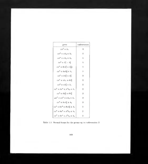
Theorem 2.1.1 L e t h G £x\ b e a g e r m s a t i s f y i n g h = h x = 0. L e t t h e c o d i m e n s i o n o f h b e l e s s t h a n o r e q u a l t o 3 . T h e n h i s E - e q u i v a l e n t t o o n e

o f t h e g e r m s i n t a b l e 1 .1 . H e r e e , 6 , d G { —1,+1} a n d f i GR \ {0} . T h e c o e f f i c i e n t f i i n t h e n o r m a l f o r m f i x 7 + e x5 + xA2 + Ai i s a m o d a l p a r a m e t e r .

Proof. It will be shown how to derive the normal forms e x 3 + S x X ^ + A] and e x 3 + xAj + 6 X \ . The other cases can be treated similarly. Also note that the germs of the form x2 + <£( A], A2) have been classified by Izumiya up to codimension five in [Izu84].

Throughout the proof fc-jets of germs g G £ x \ are written as

i k 9 = X ! v iPa?a; ,

O

Kp.q.r

1 d p + q+ rg ,

apqr ~ d x p d X xq d X 2r (° ’ ° ’0 ) '

Let £ * x denote the space of fc-jets of germs in £ x \ .

A) Consider germs in £ x \ having non-vanishing 1-jet and satisfying h =

h x = 0 . W ithout loss of generality j l h = Ai can be assumed. Now consider

2-jets of germs, whose 1-jets are equivalent to Aj . By applying M ather’s lemma [Mat70] one finds three orbits in £ 7X listed below together with their corresponding recognition conditions:

1. a2oo ^ 0 : Aj ± x2

2- «200 = 0, aioi 5^ 0 : X \ + xA;

3. «200 = 0» «loi = 0 : Aj

g e r m c o d i m e n s i o n

e x 2 +A! 0

e x 3+ xA2 + Ai 0

e x 4+ x X 2+ Aj 1

e x 2+ Aj - A| 1

e x 2+ ¿(Aj + A*) 1

e x 3+ f> x \2+ Ai 1

e x 2+ iAj + A^ 2

e x 3+ xAj + iA | 2

e x 3+ xA^ + Ai 2

£X 5 + f>x4+ x2A2 + Ai 2

e x 2+ ¿A2 + \1 X \ 3

H i 7+ ex5 + xA2 + Aj 3

ex3 + h x .X \+ Ai 3

£X 5 + ¿x4 + t i x X \+ Ai 3

£X6 + ¿x5 + x2A2 + Aj 3

e x 7+ 6 x 4 + x2 X 2 +Aj 3

Table 1.1: Normal forms for the germs up to codimension 3

Consider the last case. The orbits in for germs whose 2-jets are equiva­ lent to Ai are given by

1. 0300 ^ 0, D ^ 0 : Ai ± x3 ± x\%

2. 0300 = 0, D ^ 0: Aj + z 2A2 3. 0300i1 0, D = 0 : Ai ± x3

4. 0300 = 0, D = 0 : A] ± zA2

Here

D := 603000102 — 2o|0, .

Consider the third case. The orbits *“ ¿ l x for germs whose 3-jets are equiv­ alent to Aj ± z3 are

1. a 103 / 0 : Ai ± x3 + zA^

2- aio3 = 0 : Ai ± z3

Taking the second case one finds for the orbits in £ * x of germs whose 4-jets are equivalent to Aj ± z3 :

1. O104 ^ 0 : Aj ± z3 ± zAj

2. O]04 = 0 : A] ± z3

The second case leads to germs of codimension greater than 3. In the first case the germ A] ± z3 ± zAj *s 5-determined and has codimension 3.

B) Consider germs in £ x \ having vanishing 1-jet. Mather’s lemma yields the following orbits in

1-o2oo ^ 0, A' ji 0: ± z2+ Aj — A|, ± z2 ± (Aj + A^) 2- « 2 0 0 ^ 0 . A or D ^ 0 : ± z2 ± A2

3. a2oo ? 0. A = 0, D = 0 : ± z2

4. 0 2 0 0 = 0, L ^ 0 : zAj ± A|

5. a2oo = 0, L= 0 , Oho or flioi ^ 0 : xAi

6. 0200 = 0, a , 10 = 0 ,a,oi = 0, 2?* ± 0 : ±(A ? + A j), Af - X\

7. 0200 = 0 .« n o = 0,aioi = 0,2?* = 0, 0020 or 0002 ^ 0 : ±A3

8. 0200 = 0, Oh o = 0, a io i = 0,2?* = 0,0020 = 0,0002 = 0 : 0

Here

A := —4«020«200 + a?io >

2? := —4ooo2n2oo + «10 1 ,

K : = Oqjj O20O — «011«1 lOOlOl — 402000020fl002 + O020O101 + o f 10«002 •

L := ooo2 « ?io - a io i« o iiO n o + o j 01a 02 o , D" := Oqu — 4aoo20o20 •

Consider the fotirth case. The orbits in £ 3A of germs whose 2-jets are equiv­ alent to xAj ± A | are

1- 0300 ^ 0 : ± x3 + xAj ± Aj

2.

= 0

^ 0: xAj ± A| +

Proceeding fu rth er in the second and third case leads to germs of codimen­ sion greater th an 3. The germ ± x 3 + xAi ± A| is 3-determined and has codimension 2. □

Corollary 2.1.2 M i n i v e r s a l u n f o l d i n g s o f t h e g e r m s i n t h e o r e m 2 . 1 .1 c a n b e c h o s e n a s l i s t e d i n ta b le 1 .2 .

P ro o f. It will b e shown how to derive miniversal unfoldings for the germs

e x 7 + 6xA + x2X2 + Aj

and

ex5 + 6 x 4 -I- X 3 X2 + Aj .

g e r m u n f o l d i n g t e r m s

e x 2 + Ai

-e x 3 + xA2 + Ai

-e x 4 + xA2 + Aj X 2

e x2 + A? - \ \ 1

e x 2 + ¿(Af + A2) 1

ex3 + ¿xA2 + Ai X

e x 2 + 6 Aj + Aj i,a2

ex3 + xAi + ¿A| 1, A,

e x 3 + xAj + Ai x , xA2

e x s + 6 x 4 +x2A2 + A! x , xA2

e x 2 + ¿A? + tfAj 1, a2, A2

f i x 7 + e x5 + xA2 + A, x2 ,x3 ,x7

e x 3 + b x X \ + Ai x, xA2, xA2

ex5 + S x 4 + d x X \ + Ai x , x a, x2A2

e x 6 + 6 x 5 + x 2A2 + Ai x, xAi, xA2

e x 7 + 6 x 4 + x2A2 + Ai x, x A j.x 3

Table 1.2: Miniversal unfoldings of th e normal forms