University of Warwick institutional repository: http://go.warwick.ac.uk/wrap
A Thesis Submitted for the Degree of PhD at the University of Warwick
http://go.warwick.ac.uk/wrap/1048
This thesis is made available online and is protected by original copyright. Please scroll down to view the document itself.
Time-dependent Dalitz-Plot
Analysis of the Charmless Decay
B
0
→
K
S
0
π
+
π
−
at
B
A
B
AR
Jelena Ili´
c
Submitted to the University of Warwick for the degree of Doctor of Philosophy
University of Warwick
Department of Physics
20th
Abstract
A time-dependent amplitude analysis of B0 → K0 Sπ
+π− decays is performed
in order to extract the CP violation parameters of f0(980)KS0 and ρ
0(770)K0 S
and direct CP asymmetries of K∗+(892)π−. The results are obtained from the final BABAR data sample of (465±5)106 BB decays, collected with the
BABARdetector at the PEP-II asymmetric-energyBfactory at SLAC. The time
dependent CP asymmetry for f0(980)KS0 and ρ
0(770)K0
S are measured to be
S(f0(980)KS0) =−0.97±0.09±0.01±0.01, andS(ρ0(770)KS0) = 0.67±0.20±
0.06±0.04, respectively. In decays to K∗+(892)π− the direct CP asymmetry is found to beACP(K∗±(892)π∓) = −0.18±0.10±0.04±0.00. The relative
phases between B0 → K∗+(892)π− and B0 → K∗−(892)π+, relevant for the
extraction of the unitarity triangle angleγ, is measured to be ∆φ(K∗(892)π) = (34.9±23.1±7.5±4.7)◦, where uncertainties are statistical, systematic and model-dependent, respectively. Fit fractions, direct CP asymemtries and the
relative phases of different other resonant modes have also been measured. A
new method for extracting longitudinal shower development information from
longitudinally unsegmented calorimeters is also presented. This method has
been implemented as a part of theBABARfinal particle identification algorithm.
A significant improvement in low momenta muon identification at BABAR is
Acknowledgements
Firstly I would like to thank the Particle Physics Group at the University of
Warwick and especially to Professor Paul Harrison for giving me the
opportu-nity to study in Warwick and for providing the funding for my Ph.D.
My two supervisors: Tim Gershon and Paul Harrison for all their support,
advice and encouragement.
Many thanks to Tom Latham from whom I learnt most of the things I know
now about analyses ofB meson decays and whose knowledge of C++ and the
professional style of writing C++ software influenced me to become a better
programmer myself.
Special thanks to Pablo del Amo S´anchez, he was always ready to help and to
listen about my problems.
To Gagan Mohanty, for his enthusiasm which made a publication of our work
on the longitudinal shower development possible.
Also, to John Back, Ben Morgan John Thornby and Eugenia Puccio, they
have always made me feel as a part of the group and made the time I spent at
Warwick University enjoyable.
Finally, I would like to thank the examiners, Yorck Ramachers and Jonas
Declaration
I declare that the work in this thesis was carried out in accordance with the
Regulations of the University of Warwick. No part of the thesis has been
submitted for any other academic award at this or any other university.
The data used in this analysis were recorded by theBABARdetector run by the
BABAR Collaboration. The author contributed to the running of the detector
through the taking of detector shifts and working on the problem of the
longi-tudinal shower development in longilongi-tudinally unsegmented calorimeters. The
presented analysis is performed on the final BABAR data sample. An analysis
of the same decay channel, but on a smaller BB data sample, in which the
author was actively involved, was performed earlier. The event reconstruction
described in Chapter 3 makes use of code developed by the Collaboration,
with the packages used for 3-body B meson decay event selection (QnBUser
and CharmlessFitter) written by Fergus Wilson and Thomas Latham,
re-spectively. The software used for the likelihood Dalitz-plot fit (Laura++) was
first developed by Paul Harrison and John Back, and further extended by
Thomas Latham, Pablo del Amo S´anchez and the author. For example, the
author derived and implemented the formulae for the treatment of the tag side
interference effects, added a number of the probability density function
line-shapes and the new polar coordinate parametrisation of the isobar coefficients.
The work on the analysis described in this document (Chapters 4 and 5) was
carried out solely by the author. A new method for extracting longitudinal
shower development information (Chapter A) was developed by the author in
collaboration with Gagan Mohanty and David Brown.
Contents
Abstract i
Acknowledgements iii
Declaration v
Introduction 3
1 Theory 5
1.1 CP violation in Standard Model . . . 5
1.1.1 CP violation in decay . . . 9
1.1.2 CP violation in mixing . . . 12
1.1.3 Mixing-inducedCP violation . . . 15
1.2 Neutral B meson . . . 16
1.2.1 Time evolution of neutral B mesons . . . 16
1.2.2 Decay rate . . . 17
1.2.3 Loop and Tree diagrams . . . 20
1.3 B0 →K0 Sπ +π− and Unitarity Triangle angles . . . . 21
1.3.1 sin 2β fromB →Kππ modes . . . 21
1.3.2 Constraints onγ from B →Kππ modes . . . 24
1.4 Three-body decays . . . 28
1.4.1 Kinematics of three-body decays . . . 28
1.5 Parametrisation of the Dalitz Plot . . . 30
1.5.2 Resonance mass term . . . 32
1.5.3 Angular Distribution . . . 36
1.5.4 Blatt-Weisskopf Barrier Factors . . . 37
1.5.5 Isobar Coefficients . . . 37
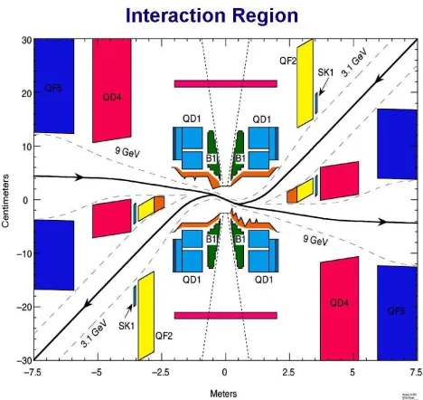
2 BABAR and PEP-II 41 2.1 The PEP-II accelerator . . . 42
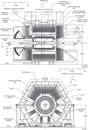
2.2 The BABAR detector . . . . 44
2.2.1 Tracking System . . . 47
2.2.2 Electromagnetic Calorimeter . . . 54
2.2.3 The Instrumented Flux Return . . . 56
2.2.4 Trigger System . . . 58
3 Analysis Techniques 61 3.1 Flavour Tagging . . . 61
3.1.1 Lepton sub-tagger . . . 64
3.1.2 Kaon sub-tagger . . . 65
3.1.3 Slow Pion sub-tagger . . . 66
3.1.4 Kaon-Slow Pion sub-tagger . . . 66
3.1.5 Highest p∗ sub-tagger . . . . 66
3.1.6 Fast-Slow correlation sub-tagger . . . 67
3.1.7 Lambda sub-tagger . . . 67
3.2 Measurement of ∆t and resolution . . . 67
3.2.1 Measurement of ∆t . . . 67
3.3 Signal and Background separation . . . 72
3.3.1 Kinematic variables . . . 72
3.3.2 Event-shape variables . . . 73
3.4 Monte Carlo Simulation . . . 78
3.5 Reconstruction . . . 81
3.5.1 Tracking algorithms . . . 81
3.5.3 Particle Identification . . . 84
3.5.4 Vertexing of candidates . . . 85
3.5.5 B Counting . . . 86
3.6 Maximum Likelihood fits . . . 86
3.6.1 Extended Maximum Likelihood fits . . . 90
3.7 The sPlot technique . . . 90
4 Analysis Method 93 4.1 Event Selection . . . 94
4.1.1 Event selection efficiency and self cross feed events . . 96
4.2 Signal Events . . . 100
4.2.1 Treatment of Self Cross Feed . . . 102
4.3 Background from B Decays . . . 107
4.3.1 BB Background PDFs . . . 115
4.4 Continuum Background . . . 118
4.5 Analysis of the discriminating variables . . . 123
4.5.1 Dependence on tagging categories . . . 123
4.5.2 Flavour dependence . . . 124
4.5.3 Dependence on Dalitz plot position . . . 125
4.5.4 Probability density functions . . . 129
4.5.5 Control sample . . . 130
4.6 Total likelihood . . . 132
5 Analysis Results and Conclusions 137 5.1 MC tests . . . 137
5.1.1 Toy MC tests . . . 137
5.1.2 Fully simulated MC tests . . . 138
5.2 Results of the fit to data . . . 139
5.2.1 sPlots . . . 141
5.2.2 Mass projection plots . . . 147
5.3 Systematic uncertainties . . . 153
5.3.1 Fixed PDF parameters . . . 153
5.3.2 ∆t parameter fluctuations . . . 154
5.3.3 Tag-side interference effects . . . 154
5.3.4 Dalitz plot histograms . . . 157
5.3.5 BB background yield fluctuations . . . 157
5.3.6 Fit biases . . . 158
5.3.7 Model errors . . . 164
5.4 Final results and conclusions . . . 168
A Longitudinal Shower Depth 173
B Pull plots of toy MC tests 181
C Fully simulated MC tests 187
D Correlation Matrix 191
List of Tables
2.1 Some final states of e+e− collisions at the Υ(4S) energy. . . . 42
3.1 Tag04 performance, as measured on the Bf lav sample. . . 63
3.2 Signal ∆t resolution parameters. . . 71
4.1 Summary of cut efficiencies evaluated on MC. . . 97
4.2 Comparison between fits to full MC with and without
separat-ing self cross feed and truth-matched events. . . 108
4.3 Dalitz-plot vetoes employed against B-backgrounds. . . 110
4.4 Summary of B+B− background. . . . 112
4.5 Summary of the B0 →(f lavour eigenstate) background modes. 113
4.6 Summary of the B0 →(CP eigenstate) background modes. . 114
4.7 Differences between MC and the data mES fit parameters for
B0 →D−π+control sample. . . . 133
5.1 Results of the fit to data for the isobar coefficients and event
yields with statistical uncertainties only. . . 150
5.2 Comparison between a+ and a− coefficients. . . 156
5.3 Systematic uncertainties - fixed signal mES and ∆E parameters. 158
5.4 Systematic uncertainties − fixed continuum background mES
parameters. . . 159
5.5 Systematic uncertainties - fixed BB¯ background mES and ∆E
5.6 Systematic uncertainties - fixed signal (B0B¯0 background)
res-olution function parameters. . . 160
5.7 Systematic uncertainties - fixed continuum background resolu-tion funcresolu-tion parameters. . . 160
5.8 Systematic uncertainties - tag side interference. . . 161
5.9 Systematic uncertainties - fixed BB¯ background Dalitz plot. . 161
5.10 Systematic uncertainties - fixed continuum background Dalitz plot. . . 162
5.11 Systematic uncertainties - fixed shape of the efficiency. . . 162
5.12 Systematic uncertainties - Dalitz plot distribution of the con-tinuum events. . . 163
5.13 Systematic uncertainties - fixed BB¯ background yields. . . 163
5.14 The uncertainties of the Dalitz plot signal model - the masses and widths of all resonances. . . 164
5.15 Dalitz plot signal model uncertainties - LASS parameters. . . 165
5.16 The uncertainties of the Dalitz plot signal model - Flatt´e pa-rameters. . . 166
5.17 The uncertanties of the Dalitz plot signal model - the Blatt-Weisskopf barrier radius. . . 166
5.18 The uncertainties of the Dalitz plot signal model - the lineshape of the ρ0(770) resonance. . . . 167
5.19 Summary of measurements of the Q2B parameters. . . 171
5.20 Results of fit to data for the isobar coefficients and event yields. 172 A.1 Comparison of pion misidentification probabilit and electron identification efficiency. . . 176
D.1 Correlation Matrix . . . 192
D.2 Correlation Matrix . . . 193
D.3 Correlation Matrix . . . 194
E.2 Theqq¯background mES PDF parameters. . . 196
E.3 The signal ∆E PDF parameters. . . 196
E.4 Theqq¯∆E PDF parameters. . . 197
E.5 Theqq¯MLP PDF parameters. . . 198
E.6 The signal MLP PDF parameters. . . 199
List of Figures
1.1 Unitarity triangle and definitions of the angles α,β and γ. . . 9
1.2 Experimental constraints on the unitarity triangle. . . 10
1.3 Example of direct CP violation. . . 12
1.4 Faynman diagram of B0−B¯0 mixing. . . . 13
1.5 Examples of tree and penguin diagrams. . . 20
1.6 New physics sensitivity of penguin diagrams. . . 21
1.7 Feynman diagrams for the B0 →J/ψK0 S decay. . . 22
1.8 sin 2βeff from penguin modes compared to the golden mode. . 23
1.9 Diagrams contributing to the amplitudes forB0 →K∗+π− and B0 →K∗0π0. . . . 24
1.10 Isospin triangles. . . 26
1.11 Example of a Dalitz plot. . . 31
1.12 Conventional (left) and square (right)B0 →K0 Sπ +π− Dalitz plots 40 2.1 Integrated luminosity. . . 44
2.2 Schematic view of the interaction region. . . 45
2.3 The BABAR detector. . . 48
2.4 End and side views of the Silicon Vertex Tracker. . . 50
2.5 Drift Chamber side view and cell layout. . . 51
2.6 dE/dx measurements in the DCH. . . 52
2.7 Diagram illustrating the operating principles of the DIRC. . . 53
2.8 Side view on the Electromagnetic Calorimeter. . . 55
2.10 Side view on the Electromagnetic Calorimeter. . . 58
3.1 Diagrams of leptonic and hadronic tagging events. . . 64
3.2 Illustration of the effect that results in the leading contribution to the correlation between the per-event errorσ∆t and the bias on ∆z. . . 70
3.3 Distributions of cosθBmom and cosθBthrust . . . 75
3.4 Distributions of the Legendre polynomials eveluated on the ROE. 76 3.5 Graphical representation of an MLP neural network. . . 77
3.6 The output of the MLP. . . 79
3.7 Schematic view of the track parameters. . . 82
4.1 Signal region and sidebands in the mES-∆E plane. . . 98
4.2 Efficiency and Self Cross Feed fraction as a function of the Dalitz coordinates. . . 99
4.3 Self Cross Feed. . . 99
4.4 Ratio of reconstructed minus true momentum over the recon-struction error for the pion candidates. . . 103
4.5 ∆E/σ∆E and mES distributions for self cross feed events. . . . 103
4.6 Average distance travelled by truth-matched and self cross feed events. . . 104
4.7 Self cross feed probability of migration RSCF. . . . 105
4.8 Self cross feed events in full MC and in toy MC generated by the implementation of the procedure described in the text. . . 107
4.9 Projection plots of the vetoed charmed and charmonium back-grounds. . . 109
4.10 Combinatorial BB background. . . 111
4.11 mES, ∆E, MLP and Dalitz plot for B+ →π0π+KS0 . . . 116
4.14 Projections on the three invariant masses of the off-peak and
on-peak sidebands data Dalitz plot distributions. . . 121
4.15 Continuum ∆t distribution modelled from the off-peak data
sample. . . 122
4.16 ThemES and ∆E dependence on tagging categories. . . 123
4.17 MLP distribution for different tagging categories. . . 124
4.18 The flavour-dependence of the signal mES, ∆E and MLP
dis-tributions. . . 125
4.19 Variation in mean and RMS of ∆E over the Dalitz plot (signal
events). . . 126
4.20 Variation in mean and RMS ofmES over the Dalitz plot (signal
events). . . 127
4.21 Variation in mean and RMS of MLP discriminant over the
Dalitz plot (signal events). . . 127
4.22 Continuum background MLP distribution dependence on the
distance from the centre of the Dalitz plot. . . 128
4.23 mES probability density functions. . . 129
4.24 ∆E probability density functions. . . 130
4.25 MLP probability density functions. . . 131
4.26 MLP probability density functions. . . 131
4.27 mES and ∆E control sample distribution. . . 134
5.1 Fully simulated MC tests. . . 140
5.2 sPlots distributions for the signal species given by the three
background discriminating variables included in the fit, mES,
∆E and MLP and the Dalitz plot variables. . . 142
5.3 sPlotsdistributions for the continuum background events given
by the three background discriminating variables included in the
fit, mES, ∆E and MLP, and the Dalitz plot variables. . . 143
5.4 Projections on the mK0
Sπ and mπ+π− invariant masses of the
5.5 Projections on the mπ+π− and mK0
Sπ invariant masses of the
sPlots Dalitz distribution for the continuum events background. 145
5.6 ∆t sPlot. . . 146
5.7 Invariant mass plots for the B0 →K0 Sπ
+π− fit. . . . 148
5.8 Invariant mass regional plots for the B0 →K0 Sπ
+π− fit. . . . . 149
5.9 Multiple solutions . . . 151
5.10 Correlations between the parameters varied in the fit . . . 152
5.11 Distributions of ∆t in f0(980)and ρ0(770)regions of the Dalitz
plot. . . 170
A.1 Schematic view of how ∆L is calculated. . . 175
A.2 Comparison of pion misidentification probabilit and electron
identification efficiency in the forward Barrel region . . . 177
A.3 Distributions of ∆L for different types of particles in different
momentum bins . . . 178
B.1 Pull plots of the signal only toy MC tests. . . 181
B.2 Pull plots of the signal only toy MC tests. . . 182
B.3 Pull plots of the signal only toy MC tests. . . 183
B.4 Pull plots of the signal, continuum background and BB¯
back-ground toy MC tests. . . 183
B.5 Pull plots of the signal, continuum background and BB¯
back-ground toy MC tests. . . 184
B.6 Pull plots of the signal, continuum background and BB¯
back-ground toy MC tests. . . 185
C.1 Fully simulated MC tests. . . 187
C.2 Fully simulated MC tests. . . 188
Introduction
There are at least three discrete transformations of general interest in particle
physics:
parity P (reflecting the space coordinates: ~x into −~x),
microscopic time reversal T (changing the time coordinatet into −t),
charge conjugation C (replacing a particle by its antiparticle).
Originally it was assumed that all three represent symmetries of nature, since
they were known to be conserved in the strong and electromagnetic processes.
The first one to lose its “true symmetry” status was parity. In 1957 it was
found that P is violated in weak processes [1, 2, 3]. The discovery led to the
conclusion that, on the microscopic level, nature distinguishes between left
and right. Soon it was realised that the idea of mirror image symmetry of
the microspace can be saved as long as the combined CP transformation is
conserved: if nature is CP-invariant, then for every process, there exists an
appropriate mirror image symmetrical process in which particles are replaced
by antiparticles, and all characteristics of both processes have to be equal.
In 1964, experimenting on decays of neutralK mesons, Christenson, Cronin,
Fitch and Turlay [4] observed the decay K0
L → π+π−, which if CP were
con-served, would be forbidden. This came as a complete surprise. Since the idea
ofCP violation was not easy to accept, a lot of scepticism regarding the
that nature distinguishes between matter and antimater and left and right was
accepted.
In the years that followed, many attempts were made in order to build a
theoretical framework for CP violation, and give an explanation for its
exis-tence. Today, we have the Standard Model which describes the CP violation
by the Kobayashi-Maskawa mechanism [7, 8], but does not explain the origin
of the CP violation, except that it is connected to the unknown coupling of
the fermions to the Higgs field. Also, almost any model of new physics, such
as supersymmetry, introduces more CP violating sources in order to generate
large CP asymmetries [9] needed for Sakharov’s explanation of baryon
num-ber asymmetry [10], i.e. the situation that today’s Universe is predominantly
populated by particles with a very small fraction of antiparticles1.
Therefore, searches for CP violation in different systems are very important
for particle physics in the sense that they may help to give the answer to the
fundamental question of the evolution of the Universe.
Charmless three-body B meson decays, such as B0 → K0 Sπ
+π−, provide a
deep insight into the nature of the CP violating processes. A rich resonance
structure and small branching fractions make them difficult to analyse, but
nevertheless the information that can be extracted from these analyses makes
it worth the effort. Thanks to the involvement of second-order weak
interac-tions, such as mixing and loop diagrams, they are among the most sensitive
low energy probes for the new physics effects. The large phase space of
three-body B meson decays provides a possibility to measure interference between
different resonant processes with more accuracy, and consequently the
possibil-ity to extract directly any phase differences involved. This provides additional
sensitivity to CP violation effects. Finally, experimental studies of
charm-less three-body B meson decays address an old, unsolved question related to
1
hadronic effects: “How to deal with nonperturbative quantum chromodynamic
effects?”.
In the thesis that follows details and results of the analysis of charmless decays
of a neutral B meson into the K0 Sπ
+π− final state, performed using the final
Chapter 1
Theory
This chapter introduces the physics ofCP violation starting with the Standard
Model formalism, after which the three scenarios forCP violation are presented
in more detail, followed by the time evolution of neutralB meson states and
general remarks about three-body decay kinematics.
1.1
CP violation in Standard Model
The part of the Standard Model (SM) Lagrangian which describes the
flavour-changing quark transitions, has the following form [11]:
Lint=−
g
√
2(J
µW+
µ +J†µWµ−). (1.1)
Here, Jµ is a V-A (vector-axial vector) charged weak current operator that couples to the W boson, W±
µ denotes the charged vector boson fields, and g
is the weak coupling constant. The V-A operator Jµ can be written in the flavour basis as:
Jµ=X
i,j
¯
uiγµ
1 2(1−γ
5)d
j, (1.2)
where, ¯ui anddj are quark fields,γµare Dirac matrices,γ5is their product and
above equation in the mass basis. Denoting the basis transformation matrix
with U:
um = Umnu u′n, dm =Umnd d′n.
Vij ≡ Umiu†Umjd , (1.3)
then Eq. (1.2) becomes:
Jµ =X
i,j
¯
ui ′
γµ1
2(1−γ
5)V
ijd
′
j, (1.4)
where the complex coefficients Vij that appear as a result of changing basis
are the elements of the CKM matrix named after Cabibbo, Kobayashi and
Maskawa [7, 8]. From Eq. (1.2) and Eq. (1.4) it can be seen that the amplitudes
for processes in which a W− boson is radiated (d
j →W−ui and ¯ui →W−d¯j)
are proportional to Vij, while the amplitudes for processes in which a W+ is
radiated (ui →W+dj and ¯dj →W+u¯i) are proportional to the Vij∗ coefficient.
In the above equation the CKM matrix appeared as a result of changing
ba-sis. Historically, this matrix was introduced to account for the experimentally
observed fact, that the weak interaction, unlike strong and electromagnetic,
does not conserve quark flavour. In other words, the CKM matrix was
intro-duced to describe the situation that there is no unique set of quark eigenstates
of weak interaction. Each up-type quark couples to a mixture of down-type
quarks. Therefore, the CKM matrix can be understood as a rotation from the
down-type quark states as seen by the strong interaction (d, s and b) to a set
of new down-type quark states as seen by the weak interaction (d′,s′ and b′):
d′ s′ b′ =
Vud Vus Vub
Vcd Vcs Vcb
Vtd Vts Vtb
d s b (1.5)
The Standard Model does not predict values of the CKM matrix elements.
They are, like fermion masses, fundamental input parameters. The only
that they are related to the fermion masses, since both have the same origin:
the unknown coupling of the fermions to the Higgs field, and unitarity
rela-tions. This Higgs-fermion interaction is usually called the Yukawa interaction.
The form of the quark-Higgs Yukawa interaction terms in the SM Lagrangian
is the following:
LY=−Yijuq¯L,iφuR,j−Yijdq¯L,iφdR,j. (1.6)
Here,Yu,dare 3×3 complex matrices, the indicesiandj label the generations,
andφ is the Higgs field. The form of Yukawa interaction terms is constrained
by SU(2)L gauge invariance, but this condition does not require the terms
to be diagonal in quark flavour. However, to determine the quark masses the
Yukawa terms have to be diagonalised. The basis in which this is accomplished
is the mass basis. As already shown in Eq. (1.3), the change from flavour to
mass basis involves the CKM matrix. Therefore, the fermion masses and CKM
matrix parameters are closely related. Together, they account for 13 of the
total 18 SM parameters (nine fermion masses, four CKM matrix elements,
three SU(3)C ×SU(2)L ×U(1)Y gauge coupling constants, Higgs mass and
vacuum expectation value of the Higgs scalar field).
The fact that the CKM matrix consists of four free parameters, three mixing
angles and one CP violating phase, can be derived from its unitarity and the
requirement that any phase has to be non-trivial (redefinition of the fields
cannot lead to the phase being zero). These may be parametrized in a variety
of ways, and perhaps the most useful parametrization is the one developed by
Wolfenstein [12], based on an empirical observation:
|Vus|3 ≈ |Vcb|3/2 ≈ |Vub|, (1.7)
unitarity and measured values of the CKM matrix elements. The Wolfenstein
representation emphasises the hierarchy in the quark couplings and expresses
matrix elements in terms of powers of λ ≡ |Vus| ≈ 0.22 [13]. Choosing a
Wolfenstein found:
VCKM =
1−12λ2 λ λ3A(ρ−iη)
−λ 1−1 2λ
2 λ2A
λ3A(1−ρ−iη) −λ2A 1
+O λ4
∼
1 λ λ3e−iγ
−λ 1 λ2
λ3e−iβ −λ2 1
. (1.8)
where the value of the parameter A is≈ 4
5, ρ≈0.15 and η≈0.35 [14], and η
is the only parameter responsible for the CP violation.
The unitarity condition (V†
CKMVCKM = I) leads to 9 relations between the
elements of the CKM matrix. For decays ofB mesons, the following equation,
which describes b→d quark transition, is of particular interest:
Vud∗Vub+Vcd∗Vcb+Vtd∗Vtb= 0. (1.9)
Since theVijare complex numbers, it is possible to interpret the above equation
as a triangle in the complex plane. This triangle is usually called the Unitarity
Triangle and is shown in Figure 1.1. To construct this particular Unitarity
Triangle Eq. (1.9) is rescaled by a factor 1
|VcdVcb∗|
. Often, instead of using
Wolfenstein’s η and ρ coordinates, ¯η and ¯ρ coordinates are used. These are
related to η and ρ according to:
¯
ρ=ρ(1−λ2/2), η¯=η(1−λ2/2). (1.10)
Many analyses have been performed to measure the magnitudes of the CKM
matrix elements. A high precision value of|Vud|is obtained from superallowed
0+ → 0+ nuclear, neutron and pion β decays. To determine a value of |V
us|
leptonic and semileptonic decays ofK0and K+, as well as semileptonic decays
of hyperons were used, while the extraction of |Vcd| and |Vcs| has been done
by analysing semileptonic D meson decays and dimuon production in deep
α = arg
−VtdVtb∗
VudVub∗
β = arg
−VVcdVcb∗
tdVtb∗
(1.11)
γ = arg
−VudVub∗
VcdVcb∗
Figure 1.1: Representation of the triangle formed from Eq. (1.9) divided by
VcdVcb∗. The definitions of the angles of the triangle in terms of the CKM
matrix elements are given on the right.
CKM matrix elements became possible with theBABARand Belle experiments.
Results for |Vcb| and |Vub| mainly come from semileptonic B decays to charm
and charmless final states, respectively, while values of couplings between d,
s and b quarks and the t quark were measured in processes with dominant
flavour changing neutral current component. Figure 1.2 shows the current
ex-perimental constraints on the sides and angles of the unitarity triangle [15]. It
can be seen that all constraints overlap nicely around the apex of the unitarity
triangle.
1.1.1
CP violation in decay
One of the simplest ways to study CP violation is to compare the decay rates:
Γ(P →f) and Γ( ¯P → f¯), where P is a pseudoscalar meson and f and ¯f are
CP-conjugate final states. If we define the action of the CP operator on the
states|Pi and |fi as:
CP|Pi=e2iθ(P)|P¯i
CP|fi=e2iθ(f)|f¯i, (1.12)
where 2θ is an arbitrary phase, and assume CP conservation in P → f
γ
γ
α
α
d
m
∆
K
ε
K
ε
s
m
∆
&
d
m
∆
ub
V
β
sin 2
(excl. at CL > 0.95) < 0
β
sol. w/ cos 2
excluded at CL > 0.95
α
β γ
ρ
-1.0 -0.5 0.0 0.5 1.0 1.5 2.0
η
-1.5 -1.0 -0.5 0.0 0.5 1.0 1.5
excluded area has CL > 0.95
ICHEP 08 CK M
[image:33.595.66.443.206.566.2]f i t t e r
A≈ hf|H|Pi=hf|(CP)†(CP)H(CP)†(CP)|Pi
=hf¯|H|P¯ie2i(θ(P)−θ(f))
= ¯Ae2i(θ(P)−θ(f)). (1.13)
Here, ¯Ais the amplitude for theCP conjugate process andH is a Hamiltonian
which commutes with the CP operator because of the assumedCP symmetry
of the decay. Therefore, whenCP is conserved:
¯
A A
= 1, (1.14)
while a situation where:
¯
A A
6= 1, (1.15)
impliesCP violation in decay. In that case, the rates Γ(P →f) and Γ( ¯P →f¯) will be different, which then can be expressed as an asymmetry:
ACP = Γ(P →f)−Γ( ¯P → ¯
f)
Γ(P →f) + Γ( ¯P →f¯). (1.16) To have an observable direct CP asymmetry more then one amplitude has to
contribute to a given decay process. The reason for that comes from the fact
that in the Standard Model, CP-conjugate amplitudes differ from the original
amplitude at most by a phase factor. In the simplest case of two amplitudes
that contribute to a given final state:
A=hf|H|Pi=
2
X
i=1
aiei(δi+φi)
¯
A=hf¯|H|P¯i=e2i(θ(P)−θ(f)) 2
X
i=1
aiei(δi−φi), (1.17)
where δi is a CP conserving (strong) phase, and φi is a CP violating (weak)
phase, the asymmetry becomes:
ACP = |A|
2− |A¯|2
|A|2+|A¯|2 =
2|a1||a2|sin(δ1−δ2) sin(φ1 −φ2)
|a1|2|+|a2|2+ 2|a1||a2|cos(δ1−δ2) cos(φ1−φ2) .
From here it can be seen that ACP will have a non-zero value only if the weak phases, as well as the strong phases, from the two processes that contribute to
the final state are different. Examples showing the interaction of the strong
and weak phases leading to appearance ofCP asymmetry are shown in Figure
1.3.
2 1
a = a + a
a = a1 1
a2
2 1
a = a + a = a*
a = a2 2*
a + a 1 2 2
a + a1
a = a1 1
a2
a 2
δ2 φ2 φ2
2 1
a = a + a
a = a1 1
a 2 2
1
a = a + a
a2
[image:35.595.62.455.206.500.2]φ2 δ2 φ2
Figure 1.3: Examples of direct CP violation. In the first case (top left) there is a relative weak phase between amplitudes a1 and a2, but no relative strong
phase. Therefore, the CP conjugate amplitude ¯a= ¯a1+ ¯a2 = a∗, and there is
noCP asymmetry. In the other two cases (top right and bottom), both, relative weak and strong phases are present, giving a CP asymmetry (a¯6=a∗).
1.1.2
CP violation in mixing
The spontaneous oscillation of a neutral meson into its antiparticle, often called
d b
0
B W W
t , c , u = q q=u,c,t qb *
V Vqd
qb * V qd V b d 0 B d b 0 B + W -W q=u,c,t q=u,c,t qb *
V Vqd
qb * V qd V b d 0 B
Figure 1.4: Box diagrams showing mixing between B0 and B¯0 mesons.
and recently was seen in D mesons [18, 19]. Mixing does not necessarily
imply CP violation, but provides interfering amplitudes that can produce CP
violation. The Feynman diagrams of mixing in theB0meson system are shown
in Figure 1.4. The particle which propagates in the loop has to be one of the
quarks with absolute charge 2/3, and therefore one of the up-type quarks.
Looking at the relevant CKM matrix elements it can be seen that any choice
of an up-quark gives a coupling of order ofλ6. On the other side, the mixing
process also includes emission and absorption of W bosons, so each vertex is
weighted by a ratio of quark and W boson masses, and therefore the t quark
loop dominates. The corresponding CKM factors are thenVtd andVtb, and the
CP violating phase (using the Wolfenstein parametrization) enters the mixing
amplitude viaVtd:
(VtdVtb∗)2 ≈e−i2β. (1.19)
So, an oscillating B0 compared to a non oscillating B0 picks up an extra
−2β phase, often called the mixing phase. This phase can be measured if both flavours decay to the same state. The standard formalism of mixing
[20] is based on a time-dependent perturbation theory analysis of a two-state
system, |P0i and |P¯0i, together with the continuum of states |fi into which
the particles P0 and ¯P0 can decay. Any state in the space of |P0i, |P¯0i and
|fi can be written as:
|Ψ(e t)i=a(t)|P0i+b(t)|P¯0i+X
f
and the Schr¨odinger equation for this system as:
id
dt|Ψ(e t)i=H|Ψ(e t)i. (1.21)
Here, H is an infinite-dimensional Hermitian matrix in the Hilbert space of
the analysed system. To solve Eq. (1.21) is a difficult task, mainly because of
insufficient knowledge of strong interaction dynamics. But, if we assume that
the initial state is a linear combination of P0 and ¯P0 alone:
|Ψ(0)i=a(0)|P0i+b(0)|P¯0i, (1.22)
and restrict ourselves to times that are much larger than a typical strong
interaction scale (Weisskopf-Wigner approximation), the Schr¨odinger equation
becomes:
H
a(t)
b(t)
=
H11 H12
H21 H22
a(t)
b(t)
=i∂
∂t a(t)
b(t)
. (1.23)
The new effective Hamiltonian matrix H is not hermitian, since we are only considering a projection onto the subspace of P0 and ¯P0.
Under the CP transformation the effective Hamiltonian H transforms in the following way:
H12≡ hP0|H|P¯0i −→ hCP P0|(CP)† (CP)H(CP)† (CP)|P¯0i
= hP¯0|e−2iθ(P)H
cpe−2iθ(P)|P0i
= e−4iθ(P) hP¯0|H
cp|P0i (1.24)
H11≡ hP0|H|P0i −→ hCP P0|(CP)† (CP)H(CP)† (CP)|P0i
= hP¯0|H
cp|P¯0i, (1.25)
where:
Hcp≡(CP)H(CP)†. (1.26)
Therefore CP is conserved if: H=Hcp, i.e.:
As a result, all CP violating observables occurring inP0−P¯0 mixing must be
functions of:
|H12| − |H21|
|H12|+|H21|
. (1.28)
In the mass basis, the above calculation becomes simpler becauseHis diagonal. If we denote the eigenvectors ofH as:
|PHi=p|P0i −q|P¯0i
|PLi=p|P0i+q|P¯0i (1.29)
after some calculation it can be found that:
|H12| − |H21|
|H12|+|H21|
=
pq
−pq
pq
+qp
. (1.30)
Therefore, CP violation in mixingoccurs if:
p q
6= 1, (1.31)
or in other words, if the physical states, which propagate in space and time
are not composed of equal amounts of particle and antiparticle states.
1.1.3
Mixing-induced
CP
violation
As shown before (Section 1.1.1) for aCP violating effect to manifest itself in
the asymmetry of the decay rates we need interfering amplitudes.
When P0 and ¯P0 mesons decay to the same final CP eigenstate (f
CP), CP
violation can occur if there is an interference between different amplitudes,
which can happen with or without mixing between the neutralP meson states.
In other words, CP violation can arise as a consequence of the interference
between decays: P0 →f
CP and P0 →P¯0 →fCP. This type of CP violation is
known asmixing induced CP violationand is the one foreseen by Bigi, Carter, Sanda and others [21] to be of primary importance in the decays of neutralB
1.2
Neutral
B
meson
1.2.1
Time evolution of neutral
B
mesons
To find how the neutral B0 and ¯B0 mesons evolve in time and space [22] we
can start by expressing the physical states of the neutral B meson in terms of
the mass eigenstates (Eq. (1.29)):
|B0i = 1
2p(|BLi+|BHi)
|B¯0i = 1
2q(|BLi − |BHi). (1.32)
The |BLiand |BHi are stationary states of the effective HamiltonianH
(Sec-tion 1.1.2). It is common to break H into its hermitian and anti-hermitian parts: H =M−(i/2)Γ, where bothM andΓare hermitian matrices, usually known as the mass and decay matrix respectively. The eigenvalues
correspond-ing to |BLi and |BHi then can be written as:
λH =MH −
i
2ΓH, λL =ML−
i
2ΓL. (1.33)
Using the above results, the time-dependence of the physical neutral B meson
states is:
|B0(t)i=e−iM t−Γt/2(cos (∆Mt/2)|B0(0)i+iq
psin(∆Mt/2)|B¯ 0(0)i)
|B¯0(t)i=e−iM t−Γt/2(iq
psin(∆Mt/2)|B 0(0)
i+ cos(∆Mt/2)|B¯0(0)i), (1.34)
where |B0(0)iand |B¯0(0)i are flavour eigenstates, ∆M = M
H −ML, M =
(MH +ML)/2 and Γ = (ΓH + ΓL)/2. The lifetime difference between the two
neutralBdmesons is very small, ∆Γ/Γ =O(10−2) [23], therefore Γ≈ΓH ≈ΓL
(the ∆Γ = 0 approximation is used to obtain the above equation), and a unit
system of c = 1, where c is the velocity of light in the vacuum, is assumed.
The previous result can be used to determine the time evolution of a B0B¯0
in a Υ(4S) decay behaves as a single entangled object. Before one of the B
mesons decays there will be exactly one B0 and one ¯B0 present, even though
they will evolve in phase according to Schr¨odingers equation.
In the Υ(4S) frame, if one of the B mesons is produced at an angle θ with
respect to the beam (z) and with azimuth angle φ, the other B meson will
be produced at an angle π −θ with respect to the beam axis and have an azimuthal angle ofφ−π. Thus, the time-evolution of the two B meson state in theΥ(4S) rest frame is given by the asymmetric term:
S(tf, tb, φ, θ) =
1
√
2[B
0(t
f, θ, φ) ¯B0(tb, π−θ, φ+π)−
¯
B0(t
f, θ, φ)B0(tb, π−θ, φ+π)] sin(θ), (1.35)
where tf and tb are the proper times of the forward and backward B mesons
respectively. Substituting Eq. (1.34) we get:
S(tf, tb, φ, θ) =
1
√
2e
(−Γ/2+iM)(tf+tb)[cos(∆M(t
f −tb)/2)(B0fB¯b0−B¯f0B
0
b)−
isin(∆M(tf −tb)/2)(
p qB
0
fB¯b0−
q pB¯
0
fBb0)] sin(θ). (1.36)
Therefore, when both physical states are present, tf =tb, so we have exactly
one B0 and one ¯B0. After one of them decays the other B meson evolves
independently by means of mixing.
1.2.2
Decay rate
To calculate the production rate for the two B meson system we need to
rewrite equation Eq. (1.36) in terms of decay amplitudes. If one of the B
mesons decays to a final statef1 at a time t1 and the other decays to the final
state f2 at time t2, the total amplitude will be:
A(t1, t2) =m(t1, t2)
1
√
2e
(−Γ/2+iM)(t1+t2)[cos(∆M(t
f −tb)/2)(A1A¯2−A¯1A2)−
isin(∆M(t1−t2)/2)( p
qA1A¯2− q
where Ai is the amplitude for a B0 state to decay to the final state fi, ¯Ai is
the amplitude for a ¯B0 state to decay to the same final state f
i and:
m(t1, t2) =
+1, t1 =tf, t2 =tb
−1, t1 =tb, t2 =tf
The modulus squared of this amplitude, integrated over all possible angles θ
gives the production rate for the twoBmeson states to produce the final states
f1 and f2. If we are interested in one particular final state (fsignal), we will
need to determine the flavour of the neutralB meson decaying into that state,
which is not a simple task since the oscillating nature of neutral B mesons
means that their flavour changes over time. But at the BABAR experiment, B0B¯0 pairs produced from the decay of theΥ(4S) resonance are entangled, so
when one of the B mesons (tagged B) decays in such a state from which the
flavour of the meson can be identified, the flavour of the other meson can be
inferred to be opposite at that exact same instant.
So, if we denote the moments when one of theB mesons decays into a
flavour-dependent state (which, for example, indicates that the flavour of that meson is
B0) and the other into the signal state, ast
tagandtrespectively, the amplitude
of B0 → f
tag as Atag and amplitude of B0 → fsignal as A, after some lengthy
calculation we can write the expression for production rate as following:
Γ(ttag, t)≈Ce−Γ(ttag−t)|Atag|2[(|A|2+|A¯|2)qtag−
qtag(|A|2− |A¯|2) cos(∆M(ttag−t))+
qtag2Im[ ¯AA∗e−iφmix] sin(∆M(ttag−t))], (1.38)
where C is an overall normalisation constant and qtag is the flavour of the B
meson decaying into a flavour-specific state:
qtag =
+1, tagged B is B0
The CP asymmetry previously defined in Section 1.1.1, in the case of neutral
B decays can be rewritten as:
Acp(∆t) = Γ (Btag=B
0(∆t)→fsignal)−Γ Btag=B0(∆t)→fsignal
Γ (Btag=B0(∆t)→fsignal) + Γ Btag=B0(∆t)→fsignal
, (1.39)
where ∆t is the time between decays of taggedB and signalB mesons. After
substituting Eq. (1.38) it becomes:
Acp(∆t) =Ssin (∆md∆t)− Ccos (∆md∆t), (1.40) where:
S = 2Imλ
1 +|λ|2 , C =
1− |λ|2
1 +|λ|2 , λ=e
−iφmixA¯
A. (1.41)
Recalling the definitions of direct and mixing-induced CP violation it can be
concluded that the coefficient S is different from zero when there is mixing-inducedCP violation, whileC 6= 0 indicates directCP violation (|A¯| 6=|A|). If there is only one SM contribution to the amplitudesAand ¯A, the expectations
are thatS =−ηCP sin (2β) and C = 0, where ηCP is the CP eigenvalue of the
final state fCP. Deviations from that imply the existence of unaccounted
amplitudes that, depending on the characteristics of the mode, could originate
from theoretical uncertainties in the Standard Model contributions, or possible
physics beyond the Standard Model.
In order to compare the experimentally measured time-dependent symmetries
among themselves and with the theoretical predictions, it is common, instead
of the mixing angle 2β, to use the effective mixing angle 2βeff [14], defined as:
S =−ηCP
√
1− C2sin 2β
1.2.3
Loop and Tree diagrams
In the Standard Model the decays of a meson containing a heavy quark
usu-ally proceed via charged-current interactions (since flavour changing neutral
currents are forbidden at the tree level) and therefore direct coupling between,
for example, the b quark and the s or d quark is not possible. The decay
amplitudes can be generally divided into two classes, called tree and penguin
(or loop) type, examples of which are shown in Figure 1.5. In the penguin
d b
+
W
1
q
2
q
d u , c
d b
+
W
t , c , u
q q
d d , s
g
Figure 1.5: Examples of tree (left) and penguin (right) diagrams. In this par-ticular case of the tree diagram quark q1 is a d or s quark, while q2 is a u or c quark. The penguin diagram is of “gluonic” type. If instead of a gluon a photon or Z0 boson is emitted from the loop the diagram is referred to as an
“electromagnetic” and “electroweak” penguin respectively.
process a quark emits and then reabsorbs aW boson, changing flavour twice,
and b →s(d) coupling is accomplished indirectly via b→t(u, c)→s(d) tran-sition. Since the b quark has no kinematically-allowed CKM-favoured decay
(Eq. (1.8)), the relative importance of the penguin decays inB meson physics
is great. The main contributor to the SM b →s penguin loop is the t quark. For this conclusion one would just has to look at the magnitudes of the CKM
matrix elements involved in the process. A similar conclusion cannot
eas-ily be made for a b → d penguin transition, since all possible SM scenarios (b→t →d,b →c→d and b→u→d) are of order O(λ3). But, the penguin
process includes emission and absorption of a W boson, so each vertex has to
domi-nant. The SM penguin loops involve heavy particles (t, W; mt = 174.2±3.3
GeV and mW = 80.403±0.029 GeV [23]), therefore rates for penguin
pro-cesses are very sensitive to non-SM extensions with heavy charged Higgs or
supersymmetric particles [24] (see Figure 1.6). Because of that measurements
of loop processes are the most sensitive low energy probes for such extensions
to the Standard Model.
b
+
H
t , c , u
s b g
~
b ~ , s ~ , d ~
s
Figure 1.6: Diagrams demonstrating the potential for new physics sensitivity in b → s penguin diagrams. On the left, a charged Higgs, predicted by, for example, the Minimal Super-symmetrical Model, enters the loop possibly car-rying a complex coupling constant. On the right, the loop formed by a gluino and (anti)squarks is shown.
1.3
B
0→
K
S0π
+π
−and Unitarity Triangle
an-gles
1.3.1
sin 2
β
from
B
→
Kππ
modes
The “golden channel” for the measurement of the Unitarity Triangle
an-gle β is B0 → J/ψK
S decay (see Figure 1.7). Theoretically and
exper-imentally it is very clean [25]. Since the top quark dominates the loop,
the CKM factors in both tree and penguin amplitudes carry approximately
the same phases, and the time-dependent asymmetry has a simple form:
The B →Kππ modes are penguin dominated b→sqq¯ transitions, where q is a u ord quark. The involved CKM matrix elements have the same phases as
those in the golden mode, and should therefore exhibit, to a good
approxima-tion, the same time-dependent asymmetries. Any significant differences could
be a result of non-SM physics appearing in the process (see Figure 1.6).
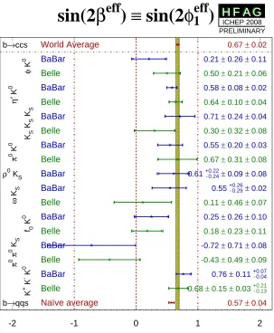
Fig-ure 1.8 shows the measFig-ured values of sin 2βeff from penguin dominated modes
compared to the golden mode. It can be seen that the penguin modes tend to
d b 0 B + W cb * ~V 2 λ ~1 cs V s c d c 0 K ψ J/ d b 0
B W+
,1 2 λ , γ i e 3 λ qb * V 2 λ ,1,-λ qs V t , c , u c c d s 0 K ψ J/
Figure 1.7: Feynman diagrams for the amplitudes contributing to the B0 →
J/ψK0
S decay.
lie on the left of the value for the golden channel. The statistical significance
of the trend is hard to determine, since the corrections are mode-dependent.
However, a na¨ıve average is less than 3σ away from the charmonium value,
and there is currently no convincing evidence for new physics effects in these
transitions. Also, the most recent results of a number of Dalitz plot
analy-ses shifted the charmless values toward the golden mode measurement, so the
differences are becoming less evident. The final state K0 Sπ
+π− allows
mea-surements of sin 2βeff in the channels B0 →f0(980)KS0 and B
0 → ρ0(770)K0 S.
Such measurements have been performed previously on smaller data samples
by isolating each resonant mode (quasi-two-body approach). A Dalitz analysis
of a larger sample can improve the quasi-two-body measurements, by
prop-erly accounting for interferences between resonances. Also, quasi-two-body
analyses are sensitive only to the interference of the state with its oscillated
counterpart, which allows a measurement of sin 2βeff, but not the angle βeff
sin(2
β
eff
)
≡
sin(2
φ
1
e
ff
)
b→ccs
φ K 0 η′ K 0 KS K S K S π
0 K
0 ρ0 KS ω K S f0 K 0 π 0 π 0 K
S
K
+ K - K
0
b→qqs
-2 -1 0 1 2
World Average 0.67 ± 0.02
BaBar 0.21 ± 0.26 ± 0.11
Belle 0.50 ± 0.21 ± 0.06
BaBar 0.58 ± 0.08 ± 0.02
Belle 0.64 ± 0.10 ± 0.04
BaBar 0.71 ± 0.24 ± 0.04
Belle 0.30 ± 0.32 ± 0.08
BaBar 0.55 ± 0.20 ± 0.03
Belle 0.67 ± 0.31 ± 0.08
BaBar 0.61 + -0 0 . . 2 2 2
4± 0.09 ± 0.08
BaBar 0.55 + -0 0 . . 2 2 6
9± 0.02
Belle 0.11 ± 0.46 ± 0.07
BaBar 0.25 ± 0.26 ± 0.10
Belle 0.18 ± 0.23 ± 0.11
BaBar -0.72 ± 0.71 ± 0.08
Belle -0.43 ± 0.49 ± 0.09
BaBar 0.76 ± 0.11 + -0 0 . . 0 0 7 4
Belle 0.68 ± 0.15 ± 0.03 +
-0 0 . . 2 1 1 3
Naïve average 0.57 ± 0.04
H F A G
H F A G
[image:46.595.170.473.130.498.2]ICHEP 2008 PRELIMINARY
Figure 1.8: sin 2βeff (the notation φ1 is also used to designate the
Unitar-ity Triangle angle β, notably by the Belle Collaboration) from penguin modes compared to the golden mode. The comparison is made by the Heavy Flavour Averaging Group [26] after the 2008 Summer conferences.
resonances with the oscillation amplitude, which enables the determination of
1.3.2
Constraints on
γ
from
B
→
Kππ
modes
Recently published papers [27, 28] pointed out the possibility of using Dalitz
plot analyses of B →Kππ decays to extract the angle γ, the most poorly determined angle of the unitarity triangle, γ = 7027
−29
◦ [15].
The currently favoured methods for γ measurement are based on the
inter-ference between the colour-allowed B− → D0K− and the colour-suppressed
B− →D0K− decay modes. In these decays only tree amplitudes are present, which makes them theoretically very clean, but the small relative magnitude
of the two amplitudes (0.046.rB .0.126) [14] reduces the sensitivity to γ.
d b 0 B + W ub * ~V γ i e 3 λ λ ~ us V s u d u *0 K 0 π d b 0 B + W ,1 2 λ , γ i e 3 λ qb * V 2 λ ,1,-λ qs V t , c , u d d d s *0 K 0 π d b 0 B ub * ~V γ i e 3 λ λ ~ us V + W s u d u *+ K -π d b 0 B + W ,1 2 λ , γ i e 3 λ qb * V 2 λ ,1,-λ qs V t , c , u u u d s *+ K -π
Figure 1.9: Diagrams contributing to the amplitudes forB0 →K∗0π0 (top) and B0 → K∗+π− (bottom), with the tree diagrams on the left, and the penguin diagrams on the right. The tree diagram for B0 → K∗+π− is an external emission tree, while the B0 →K∗0π0 is an internal emission tree.
The new method proposed by Ciuchini, Pierini and Silvestrini [27] and Gronau,
Pirjol, Soni and Zupan [28] is based on the possibility of the Dalitz plot
tech-nique to extract relative phases. That, combined with isospin symmetry of the
isospin symmetry amplitudes for these processes can be written as:
A K∗+π− = P˜+ ˜Ee (1.43)
A K∗0π0 = √−1
2 ˜
P + √1
2 ˜
Ei, (1.44)
where ˜P is the penguin amplitude, while ˜Ei and ˜Ee are internal and external
emission tree amplitudes. With the help of the unitarity triangle relation
V∗
tbVts +Vcb∗Vcs +Vub∗Vus = 0, the penguin amplitude can be separated into
CKM-favoured (P;t quark loop) and CKM-suppressed (PGIM;u and c quark
loops) parts, and the above equations can be rewritten as:
A K∗+π− = Vtb∗VtsP −Vub∗Vus Ee−PGIM
(1.45)
√
2A K∗0π0 = −Vtb∗VtsP −Vub∗Vus Ei+PGIM
. (1.46)
Since the amplitude for theCP-conjugateB0 process is obtained by
complex-conjugating the CP-odd phases (i.e. the CKM factors), when combined with
the above relations the penguin terms cancel and the following can be written:
A0 = A K∗+π−+√2A K∗0π0
= −Vub∗Vus(Ee+Ei) (1.47)
¯
A0 = A K∗−π++√2A K∗0π0
= −VubVus∗ (Ee+Ei), (1.48)
from where the ratio of amplitudes A0 and ¯A0 can be calculated:
R0 = A¯
0
A0 =
VubVus∗
V∗
ubVus
=e−i2γ
γ = −1
2argR
0. (1.49)
Therefore, to measure the CKM angleγ one has to measure the relative phase
between amplitudesA0 an ¯A0. In quasi-two-body approaches, only the
Dalitz plot approach allows not only the measurement of relative magnitudes,
but also of relative phases.
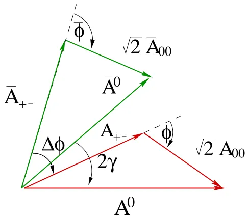
In Figure 1.10 a graphical representation of Eq. (1.47) and Eq. (1.48) is shown.
From there one can see that the value of the UT angle γ can be extracted if
angles φ, ¯φ and ∆φ are known. Angles φ and ¯φ can be determined from the
three-body decay of B0 → K+π0π− as relative phases between A
+− and A00 amplitudes and ¯A+− and ¯A00, respectively, where Aij denotes amplitudes of
B0 →K∗iπjprocesses. The angle ∆φcan be measured in a Dalitz plot analysis
of B0 →K0
Sπ+π− decay, considering the decay chainB0 →K∗+(→K0π+)π−
and the CP conjugate ¯B0 → K∗−(→ K¯0π−)π+. These two decay channels
do not overlap in the Dalitz plot, but they both interfere with the decays
B( ¯B)→ ρ0(→π+π−)K
S and with other resonances contributing to the same
Dalitz plot, from which the phase between theK∗+π− and K∗−π+ resonances
can be calculated.
A
+
2 A
00
A
0
2 A
00
A
0
A
+
φ
φ
∆φ
[image:49.595.137.380.402.617.2]2γ
Figure 1.10: Graphical representation of Eq. (1.47) and Eq. (1.48). The value of the UT angleγ can be calculated if anglesφ,φ¯and∆φare known. These can be measured in the Dalitz plot analysis of B0 →K+π0π− and B0 →K0
Sπ+π−
The above calculations have been simplified by not taking into account the
electroweak penguin contributions (obtained by exchanging the gluon in the
penguin diagrams with a photon). Considering the full (weak, strong and
electromagnetic) effective Hamiltonian for the transition, the authors of [27]
give the following final expression:
R0 =e−i(2γ+arg(1+κEW))×(1 + ∆), (1.50)
where ∆ is theoretically bound (.0.05) andκEW is:
κEW =
3 2
CEW
+ C+
1 + 1−λ
2
λ2(ρ+iη) +O λ 2
, (1.51)
with CEW
+ and C+ being, respectively, the coefficients of the electroweak and
normal QCD 4-quark operators in the effective theory. κEW is found to be an
O(1) correction to the decay amplitude of the isospin 3/2 final state. Using available results on B0 → K+π0π− and B0 → K0
Sπ+π− Dalitz plot analyses
the authors found that the value of the UT angleγ should be between 39◦ and 112◦ and placed the following CKM constraint:
¯
η= tanγ[¯ρ−a±b]. (1.52)
Here a=0.24 is the electroweak penguin correction and b = 0.03 the error of
the electroweak penguin model.
The uncertainty of the UT angle γ, obtained using the described method,
is rather large compared to the result obtained using the B− → D0K− and
B− → D0K− analyses. The reason for this lies in large uncertainties of φ, ¯
φ and ∆φ angles. Therefore, more precise analyses of B0 → K+π0π− and
B0 → K0
Sπ+π− decays are needed in order to improve the precision of the
method, which justifies a Dalitz plot analysis of theB0 →K0 Sπ
+π− decay on
1.4
Three-body decays
1.4.1
Kinematics of three-body decays
In the case of aBmeson decay to three scalar particles: B →a1+a2+a3, there
are several kinematic constraints which reduce the number of independent
variables needed to describe the process to only two. The usual choice is the
two squared invariant masses m2
ij = p2ij, where pij = pi +pj, and pi is the
four-momentum of particle i.
In this case, the conservation law of four-momentum gives the following
rela-tion:
m212+m213+m223=mB2 +m21+m22+m23, (1.53)
and in the B meson rest frame:
m2ij = (pB−pk)2 =m2B+m2k−2mBEk
m2ij = (pi+pj)2 =m2i +m2j + 2EiEj−2|p~i||p~j|cosθij, (1.54)
wherek 6=i, j, andθij is the angle betweenp~iandp~j. From the above equations
it can be concluded that the energies of daughter particles depend only on the
invariant masses of the pairs of daughter particles and also that the relative
orientation of the daughter particles’ momenta is fixed for known energies,
lying in a plane in the B meson rest frame.
The Lorentz invariant phase space for such a decay can be written as:
dN = δ4 pB−
3
X
i=1
pi
! 3
Y
i=1
d3p
i
(2π)32E
i
≈ δ mB−
3
X
i=1
Ei
! p2
1dp1p22dp2
2E12E22E3
dΩ1Ω1−2, (1.55)
where mB and pB are the mass and momentum of the decaying particle
re-spectively, pi and Ei are the momenta and energies of the daughter particles,
of p~2 with respect to p~1. When the decaying particle is a B meson, its scalar
nature leads to a uniform distribution of the decay system, and therefore the
direction of one daughter particle’s momentum (say ~p1) can be fixed, which
gives R dΩ1 = 4π, and
R
dΩ1−2 = 2πdcosθ12, where θ12 is the angle between ~
p1 and p~2. Using:
E3 =
q p2
3+m23 =
q p2
1+p22+ 2p1p2cosθ12+m23, (1.56)
equation Eq. (1.55) can be rewritten as:
dN ∝ δ
mB−E1−E2−
q p2
1+p22+ 2p1p2cosθ12+m23
×
dcosθ12 p2
1dp1p22dp2 E1E2E3
. (1.57)
Once integrated, this becomes:
dN ∝ E3
p1p2 p2
1dp1p22dp2 E1E2E3
= p1dp1
E1
p2dp2 E2
. (1.58)
Finally, since EidEi =pidpi, and (from Eq. (1.54))dEk =−dm2ij/mB:
dN ∝dE1dE2 ∝dm212dm223. (1.59)
Thus, the decay rate of a three-body decay is:
Γ =|M|dN ∝ |M|dm212dm223, (1.60) where |M| is the matrix element for the decay, which holds all information about the decay’s dynamics. From the above equation it can be seen that
the dynamics of a three-body decay can be visualised by a scatter plot in
any two of three m2
ij variables. Such a plot is often called a Dalitz plot [29].
If |M| is a constant, the Dalitz plot will have a uniform distribution as the decay proceeds according to phase space only. A distribution which is not
uniform indicates a matrix element which has a kinematic dependence, such
as an intermediate resonant decay. A resonance will appear as a narrow band
![Figure 1.2: Experimental constraints on the sides and angles of the unitaritytriangle, by the CKMfitter group [15], updated with the results available insummer 2008.](https://thumb-us.123doks.com/thumbv2/123dok_us/9729661.473874/33.595.66.443.206.566/figure-experimental-constraints-unitaritytriangle-ckmtter-updated-available-insummer.webp)

![Figure 1.11: Toy Monte Carlo simulation off B0 → K0Sπ+π−. The resonances0(980), ρ0(770), K∗(892) and K∗0(1430) have been included, approximately inthe proportions found by Belle [30].](https://thumb-us.123doks.com/thumbv2/123dok_us/9729661.473874/54.595.131.501.112.366/figure-monte-carlo-simulation-resonances-included-approximately-proportions.webp)

![Figure 2.6: dE/dx measurements in the DCH shown as a function of trackmomentum. The overlaid curves are Bethe–Bloch predictions calculated fromcontrol samples of each of the labelled particle types [47].](https://thumb-us.123doks.com/thumbv2/123dok_us/9729661.473874/75.595.157.362.103.304/measurements-function-trackmomentum-predictions-calculated-fromcontrol-labelled-particle.webp)
