Grid scale fluctuations and forecast error in wind power

(1)

warwick.ac.uk/lib-publications

Original citation:

Bel, G., Connaughton, Colm, Toots, M. and Bandi, M. M.. (2016) Grid-scale fluctuations and

forecast error in wind power. New Journal of Physics, 18 (2). 023015.

Permanent WRAP URL:

http://wrap.warwick.ac.uk/79431

Copyright and reuse:

The Warwick Research Archive Portal (WRAP) makes this work of researchers of the

University of Warwick available open access under the following conditions.

This article is made available under the Creative Commons Attribution 3.0 (CC BY 3.0) license

and may be reused according to the conditions of the license. For more details see:

http://creativecommons.org/licenses/by/3.0/

A note on versions:

The version presented in WRAP is the published version, or, version of record, and may be

cited as it appears here.

(2)

This content has been downloaded from IOPscience. Please scroll down to see the full text.

Download details:

IP Address: 137.205.202.97

This content was downloaded on 02/06/2016 at 16:43

Please note that terms and conditions apply.

Grid-scale fluctuations and forecast error in wind power

View the table of contents for this issue, or go to the journal homepage for more 2016 New J. Phys. 18 023015

(3)

New J. Phys.18(2016)023015 doi:10.1088/1367-2630/18/2/023015

PAPER

Grid-scale

ﬂ

uctuations and forecast error in wind power

G Bel1_{, C P Connaughton}2_{, M Toots}3_{and M M Bandi}3

1 _{Department of Solar Energy and Environmental Physics, Blaustein Institutes for Desert Research, Ben-Gurion University of the Negev,} Sede Boqer Campus 84990, Israel

2 _{Centre for Complexity Science, University of Warwick, Coventry CV4 7AL, UK}

3 _{Collective Interactions Unit, Okinawa Institute of Science and Technology Onna, Okinawa, 9040495, Japan} E-mail:[email protected]

Keywords:wind power, correlations, turbulence

Abstract

Wind power

ﬂuctuations at the turbine and farm scales are generally not expected to be correlated

over large distances. When power from distributed farms feeds the electrical grid,

ﬂuctuations from

various farms are expected to smooth out. Using data from the Irish grid as a representative example,

we analyze wind power

ﬂuctuations entering an electrical grid. We

ﬁnd that not only are grid-scale

ﬂuctuations temporally correlated up to a day, but they possess a self-similar structure

—

a signature of

long-range correlations in atmospheric turbulence affecting wind power. Using the statistical

structure of temporal correlations in

ﬂuctuations for generated and forecast power time series, we

quantify two types of forecast error: a timescale error

(e

t

)

that quantiﬁes deviations between the high

frequency components of the forecast and generated time series, and a scaling error

(e

z

)

that quantiﬁes

the degree to which the models fail to predict temporal correlations in the

ﬂuctuations for generated

power. With no

a priori

knowledge of the forecast models, we suggest a simple memory kernel that

reduces both the timescale error

(e

t

)

and the scaling error

(e

z

)

.

1. Introduction

Renewable power generation, unlike conventional power, exhibits variability owing to naturalfluctuations in the energy source[1], withfluctuation time scales depending on the source type. Whereas biomass and hydroelectric sources vary over long time periods, wind and solar photovoltaics exhibit short time scale variability. Wind power, in particular, shares the spectral features of the turbulent wind from which it derives energy at the scales of an individual turbine[2]and a wind farm[3,4]. This spectral correspondence implies that correlations of atmospheric turbulence are reflected in the temporal correlations offluctuations in the generated wind power. One normally assumes that geographically distant wind farms are independent and that temporal correlations in thefluctuating wind power for each farm do not translate into long-range spatial correlations. The total power entering the grid from a large number of distant farms is expected to be much smoother and to exhibit much weaker high frequencyfluctuations[5]than the power entering from a single wind farm or a single turbine. This assumption forms the basis for proposals to interconnect local wind farms[6]for the purpose of mitigating wind powerfluctuations[5]. Whereasfluctuations do smooth out as an increasing number of wind farms contribute to the aggregate power, it has been shown that thefluctuations are still larger than expected[7].

Using data from the Irish grid operator EIRGRID[8]as a representative example, we studied the temporal correlations in the aggregate wind power entering the Irish grid. The Irish grid is fed by 224 wind farms[9]

spread across the Republic of Ireland, a much larger number of farms than the number in the aggregate power previously considered in Texas[7]. We found that the aggregate wind power entering the Irish grid exhibits temporally correlatedﬂuctuations with a self-similar structure. The persistence of correlations, despite an order of magnitude increase in the number of wind farms(and their spatial distribution), strongly points to the presence of long-range spatial correlations in the atmospheric turbulence, which couples geographically distributed wind farms, thereby rendering them non-independent. These results accord with prior studies establishing the presence of long-range correlations within the mesoscale(∼1–1000 km)of atmospheric OPEN ACCESS

RECEIVED 18 September 2015

REVISED 15 November 2015

ACCEPTED FOR PUBLICATION 4 January 2016

PUBLISHED 1 February 2016

Original content from this work may be used under the terms of theCreative Commons Attribution 3.0 licence.

Any further distribution of this work must maintain attribution to the author(s)and the title of the work, journal citation and DOI.

(4)

turbulence[10]. For long time scales, theseﬂuctuations in atmosphericﬂows were shown to exhibit a multi-fractal structure[11].

Variability adds a cost to renewable power[12,13]that is absent in conventional power generation. Since an electrical grid has no storage capacity, the production and consumer demand must be balanced in real time at every instant. The grid operator purchases energy units from the producer4, in an energy market, from a few days to a few milliseconds in advance of delivery. With conventional energy, the grid operator must estimate in advance the consumer demand(scheduling), the estimation of which may not be trivial, and additional energy units required on standby(operating reserves). In the case of renewable energy, the operator must additionally account for both variability(ﬂuctuations)and forecast uncertainty(error)at the production end, calling for uncertainty management[14]in scheduling. Furthermore, large ramps in powerﬂuctuations, in the case of renewable energy, present the possibility of grid destabilization[15]and blackout, a constant source of concern for grid operators[5,16]. This risk further increases the cost of the operating reserves[17]needed on standby to prevent grid failure[18]. Naturally, forecast models constitute essential tools in estimating the magnitude of

ﬂuctuations beforehand and in planning for the optimal operating reserves required on call. Yet, no standards for forecast accuracy currently exist[19].

The performance of a model is often quantified by the mean and variance of the error(deviation of the prediction from the measured value). Extant works on wind power forecast error, ranging from the turbine to the grid scale, have focused on modeling the forecast error distribution[20–25]. Since a probability distribution is time-independent, it contains no information on temporal error variations. Several studies have considered the dependence of the mean and variance of the error on the duration for which the power is predicted(ranging from minutes to hours)[26,27]. Other works have considered the different distributions of errors for mean power over different durations5[22,23]. However, none of these studies account for thefluctuation correlations of the atmospheric turbulence[28]transferred to the generated power in the analysis of forecast error or for the temporal correlations in thefluctuations and errors themselves. Here, we suggest that the performance of wind power forecast models(as well as the performance of any model for non-stationary processes)should also account for the quality of the prediction against temporal correlations.

To analyze temporal correlations in grid-scaleﬂuctuations for wind power, we draw upon the Statistical Theory of Hydrodynamic Turbulence to quantify two types of forecast error. Theﬁrst is a timescale error(et)

that quantifies the timescales over which the forecast models fail to predict high frequency powerfluctuations. This timescale error sets a bound on the numerical resolution of forecast models and would already be known to producers who own the farms and run the forecast models. However, model details are usually not available to grid operators(see footnote 1,[29])who manage the supply side uncertainty[14]. The second type of error we quantify is a scaling error(ez)that establishes a difference in the self-similar scaling offluctuations as observed for actual generated power vis à vis the power that was forecast to be generated. This error could be potentially useful to model developers, and if such an error results from large-scale correlations in atmospheric turbulence, incorporating these correlations into models is not subject to limitations arising from numerical resolution. Having established the errors, we employ a simple memory kernel upon the forecast time series and show that the errors are easily reduced with a minimal computational cost.

Two raw time series are provided by EIRGRID: the wind power generated nationwide across all Ireland entering the grid pg(t), and the power forecast by EIRGRID’s modelspf(t)for the same period. The forecast is provided for 24 h at a time(implying different lead times for different times in the forecast series)and is based on a multi-scheme ensemble of regional weather forecast models[30,31]. The time series sampled at 15 min intervals span afive-year period(2009–2014). As we discuss in the following, we observed no change in the forecast accuracy during thisfive-year period. Given that most spot markets6do not trade at time scales shorter than 15 min[32], our analysisfinds potential applicability in these markets, as well as in managing uncertainty over a future horizon of several hours up to a day to improve forecast models.

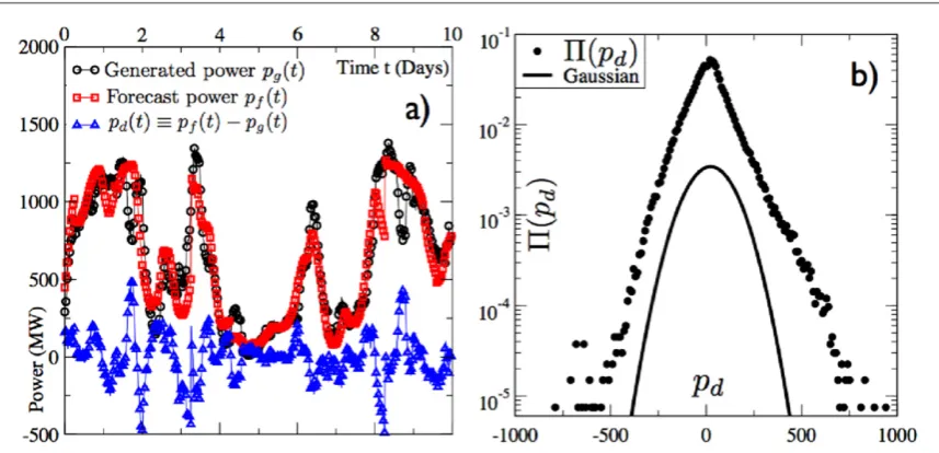
Raw time series for the generated power pg(t), forecast power pf(t), and their instantaneous difference p t_d( )ºp t_f( )-p t_g( ), which we define as the instantaneous forecast error, are shown infigure1(a)for a 10 d period, permitting a few immediate qualitative observations. Firstly,pg(t)exhibits correlatedfluctuations. Secondly,pf(t)while closely following pg(t), misses the high frequency(relative to the sampling rate of the time series)components. The instantaneous forecast errorPd(t)exhibits correlatedfluctuations and its kurtosis

5.8

4 4

kºm s » (_m₄_º ₍p_d_-p_d₎4_, 2 _p _p d d2

( )

s º - , andp_drepresents the time average of the instantaneous error), implying a broader than Gaussian distribution(k=3for a Gaussian distribution)of the instantaneous error as is evident fromﬁgure1(b).

4

For Ireland, EIRGRID is both the producer and distributor of wind power.

5

Note that[22]suggests the Cauchy distribution for the errors. However, this distribution is not suitable because all its moments are undeﬁned[47].

6

(5)

2. Data analysis

The time series were analyzed in two stages, with trends in the series being identified in thefirst stage, followed by an analysis of thefluctuations around the trends in the second stage. Trend removal permits a focus on

systematic differences betweenpg(t)andpf(t)ignoring differences due to new wind farms and the seasonal variability of the wind power. The trend identiﬁcation employed here is based on a fast Fourier transform(FFT) analysis of the time series. FFTs of the generated and forecast power time series were obtained, and the

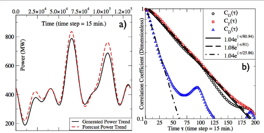
frequencies were ranked by their amplitudes(large to small, for each series separately). New time series were obtained by inverting the FFTs, keeping only thefirstmfrequencies(those with the largest amplitudes)and setting the amplitudes of all other frequencies to zero(the amplitudes of the zero frequency components were unchanged in order to preserve the signal mean in the trends). The trends were defined as the time series (obtained by the procedure described above)such that the cross-correlation between the series obtained from the generated and forecast power is maximal. Keeping the original amplitudes of the zero frequency(to preserve the signal mean)andfive more frequencies resulted in a peak cross-correlation of 0.9904 between the generated and forecast power trends(figure2(a)). These respective trends were subtracted from the raw time series. We denote the detrended generated power byPG(t), forecast power by PF(t)and their instantaneous difference by PD( )t ºP tF( )-P tG( ). The frequencies with the maximal amplitudes that were used in the trends correspond to periods of 231–1389 d, implying that the high frequencyfluctuations were not affected by our detrending procedure. We emphasize that within the aforementioned protocol, the diurnal oscillation frequency was not explicitly removed from the time series(we elaborate on this point in section5.).

The characteristicfluctuation timescales for the detrended time series werefirst computed from their respective autocorrelation functions defined as:

C P t P P t P

P t P , 1

X X X X X

X X 2

( ) ( ( ) )( ( ) )

( ( ) ) ( )

t = - +t

-wherePXis a time-average subtracted from the signal(our detrending renders a zero signal mean since the zero frequency component was preserved in the trend and removed from the detrended series). The subscriptX

should be replaced with G for generated power, F for forecast power, and D for instantaneous forecast error, respectively. The three autocorrelation functions(ﬁgure2(b))exhibit exponential decay for short times with a dataﬁt following the functional formCX( )t ~AXe-(t tX), where AX 1.0, owing to CX( )t being

[image:5.595.122.551.61.268.2]

normalized, andtXrepresents the characteristic decorrelation time for each time series, yieldingtG=80.94 data points(∼20.24 h)for generated power,tF=81points(also∼20.24 h)for forecast power, andtD=25.86 points(∼6.5 h)for instantaneous forecast error. Different detrending schemes, i.e., using different numbers of frequencies in the trend(the parametermdeﬁned above), resulted in decorrelation times in the range of 19.5–28 h. However, we found that for all the values ofmthat we tested,tFtGand the same trend of a shorter decorrelation time for largermwas found in both the detrended generated and the forecast power. This trend is

Figure 1.(a)Raw time series(for 10 d)of the generated powerpg(t) (black empty circles), forecast powerpf(t) (red empty squares), and the instantaneous forecast errorpd(t) (blue empty triangles)in megawatts(MW). Every third data point is plotted for easy visibility.(b)The probability density function of the raw instantaneous forecast error P( )p_d (black full circles)has exponentially decaying tails that are broad relative to a Gaussian distribution(solid black line)of the same mean and standard deviation as P( )p_d . The Gaussian distribution is vertically shifted for easy comparison.

3

(6)

expected because the larger them, the larger the deterministic fraction of the signal that is removed in the detrending procedure. The shortest decorrelation time reﬂects the inherent nature of theﬂuctuations. The detrended series were also split into independent time series of shorter duration(1/8th of the original temporal duration). Autocorrelation functions computed for these windowed data did not reveal a measurable difference in the characteristic decay timetX;deviations were apparent only for long-term behavior, spanning a week(or longer timescales), when the decorrelation had already occurred. The correlation time of high frequency

fluctuations(20 h)is much shorter than the slow varying trend(over months to years). Hence the detrending protocol(in particular, the number of maximal amplitudes)does not influence the analysis to follow-a fact verified and reported upon later. Analysis of the instantaneous forecast errorPD(t)for the eight independent time series of shorter duration did not reveal a measurable change in thefluctuations(mean and standard deviation), suggesting that the forecast accuracy remained the same over the consideredfive-year period.

Autocorrelation functions for the generated(CG( )t )and forecast(CF( )t )power exhibit nearly identical scaling and the same characteristic decay timescales(tG =tF=20.24h), suggesting the accurate capture of

correlations in generated power by the forecast models. Yet, the autocorrelation function CD( )t for instantaneous forecast error PD(t)informs us that some correlations are not captured. In particular, we

qualitatively know thatPF(t) misses the high frequency components ofPG(t), and they end up inPD(t), thereby contributing to its two-point correlator. This correlation deﬁcit suggests that the higher order moments of the two-point correlator are necessary to capture the statistical structure of the missingﬂuctuations.

3. Temporal structure functions

Statistical analysis of higher order correlations is a well-developed, mature tool within the statistical theory of hydrodynamic turbulence in which higher order two-point correlators are studied throughstructure functions. Kolmogorov’s theory of 1941(K41)[33]lays the foundation for structure functions through the celebrated‘4/5 law’:S r3( ) º á D( v r( ))3ñ º á( (v R+r)-v R( ))3ñ = -₅4er, where the third moment of longitudinal velocity differences(_{á D}₍ v r_{( ))}3_ñ₎_{between two points spatially separated by a longitudinal distance}_r_is proportional to the product of the average turbulent dissipation rate(e)and the longitudinal spacingr[34].

Thenth order structure function encodes all cross-terms up to ordernof the two-point correlator for a given stationary signal. The physical relevance of structure functions may be appreciated by considering a stationary,

[image:6.595.122.548.62.277.2]

ﬂuctuating signalx(t)with a zero mean. The difference between two values of this signal taken timeτapart (Dx( )t ºx t( +t)-x t( ))is collected at various windows(of durationτ)along the time series.Dx( )t is therefore a random variable with statistics of its own, and thenth order structure function, deﬁned as Sn( )t = á D( x( ))t nñ, is thenth moment for its probability density function(PDF)P D( x( ))t . The moment

Figure 2.(a)Theﬁve-year trends forpg(t) (solid black line)andPf(t) (dashed red line)are subtracted from the raw time series in subsequent analysis.(b)Log-linear scale: autocorrelation functions CG( )t (empty black circles),CF( )t (empty red squares)and

CD(t) (empty blue triangles)forPg(t),PF(t)andPD(t), respectively, exhibit exponential decorrelation with respective characteristic timescales obtained from theﬁt to data oftG=80.94points(20.24 h),tF=81points(20.24 h)andtD=25.86points(∼6.5 h).

(7)

Sn( )t varies with the time differenceτbetween signals, and its scaling, if any, reveals temporal variations in the statistical structure of theﬂuctuations of the signal to thenth order.

Tails of the PDFP D( x( ))t exert themselves with increasing ordernof the structure function, thus necessitating more data to resolve higher order structure functions. A weak test for resolving thenth order structure function involves splitting the time series into smaller windows and testing for identical scaling on the truncated series. However, this test only ensures the stationarity of the statistics. A strong test for the ability to resolve thenth order structure function requires thatﬁrst, the moment’s integrand₍_Dx₎n_{P D}₍ x₎_0_as

x

∣D  ¥∣ [35](required due to theﬁniteness of the data), and second, the PDFP D( x)should decay faster than1 _∣_Dx_∣n+1_for_∣_{D  ¥}_x_∣ _{or else the integral}

_ò

₍_D_x₎n_{P D}₍ _x₎ _d_x_{would diverge for large}_∣_D_x_∣_[₃₆_]₍_{test for} the existence of a PDF’snth moment).Whereas the two conditions are not independent, the second condition is theoretical and does not depend upon the available statistics. When conducting data analysis, even when the second condition is satisfied, insufficient data can lead to noise and prevent the integrand₍_Dx₎n_{P D}₍ x₎_from satisfactorily converging to zero[37]. Thefirst condition is, therefore, dependent on thefiniteness of the data. Based on both weak and strong tests, we conclude that the EIRGRID data can resolve structure functions up to ordern=12; however, we only present results up ton=10. Forn10, tails of the integrand₍_Dx₎n_{P D}₍ x₎ become noisy. Despite the convergence of the integral, the noise amplitude begins to compromise the quality of the structure functions(e.g. please seefigure 4 in[38]and related discussion therein)as can be observed in

ﬁgure3(a) forn=10.

Since even-order structure functions take only positive values, they converge faster than ones with odd order. To overcome this distinction between odd and even orders, we compute thenth order structure function of the absolute value of differences:SnX( )t º á∣P tX( +t)-P tX( )∣nñ, where subtraction of meanP tX( +t) andP tX( )is assumed. While ensuring the same convergence rate for even- and odd-order statistics, it also collates all data in the positive quadrant, permitting easy visualization.

4. Results

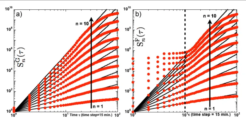
[image:7.595.121.552.62.271.2]

Figure3plots the structure functions of ordern=1–10 for the absolute value of the signal differences of the generated power∣D(PG( ))∣t (ﬁgure3(a))and the forecast power∣D(PF( ))∣t (ﬁgure3(b)). Self-similar or power-law scaling is observed for the generated power structure functions over 1.4 decades spanningt40. Scaling over the same temporal range is also observed for the forecast power structure functions of ordern=1 and 2. Forn>2, no scaling is observed for timescalest10. The scaling is restored over a limited range of timescales10< <t 40 (0.4 decades in time).

Figure 3.Structure functions of ordern=1–10(solid red circles)and their power-lawﬁts(solid black lines)for(a)generated power SnG( )t and(b)forecast powerSnF( )t plotted versusτin log–log scale exhibiting self-similar scalingSnX n

X ( )t µtz (X is G for generated and F for forecast power). The scaling is robust for(a)the generated power over 1.4 decades(40 time steps).(b)In contrast, for forecast power, theﬁrst- and second-order structure functions exhibit scaling up tot=40 time steps, but forn>2, no scaling is observed fort10 time steps. Self-similar scaling is restored over a limited range of timescales10< <t 40.

5

(8)

Self-similar scaling of the temporal structure functions implies a relationship of the form:

SnX AnX n, 2

X

( )t µ tz ( )

wherez_nXis the scaling exponent. For simple mono-fractal scaling,z_nXµn. However,ﬂuctuations with a multi-fractal character exhibit a nonlinear dependence of the scaling exponentz_nXwith respect ton. Super-(sub-) linear variation ofz_nXversusnimplies the temporal expansion(compression)ofﬂuctuations[39]. Scaling exponents for all the structure functions were computed from the log derivative, _n d S

d

X log

log

nX

( ( )) ( )

z = _tt , which provides a more reliable estimate of the exponent than a power-lawﬁt[40,41]. The pre-factor AnXin equation2is

subsequently obtained from aﬁt to the data. Inﬁgure3, all the data(solid red circles)were divided by AnXsuch

that allﬁts(solid black lines)commence from both mantissa(τ)and ordinate(SnX( )t )at unity, for an easy comparison ofz_nXwith ordern. All the data inﬁgures3,4(a)and5(b), therefore, follow the scaling relation:

S_nX n

X

( )t µtz (A_nX º1).

The scaling infigure3reveals higher order temporal correlations at work in the EIRGRID data. The absence of scaling forS_nF( )t forn>2at timescalest 10confirms the qualitative observation made infigure1(a)that forecast models do not capture high frequencyfluctuations. More importantly,figure3(b)ascribes a precise bound on the time(t=10,2.5 h)up to which the high frequencyfluctuations are missed. Finally, the scaling presence forS_nF_{( )}_t , n ₌ 1, 2_{explains the close agreement between the autocorrelation functions} _C

G( )t and CF( )t and their identical characteristic decay times,tGandtF, observed inﬁgure2(b). This is to be expected on the grounds that the second-order structure functionS2( )t º

x 2 x t 2 x t 2 2 x t x t

( ( ))t ( t) ( ) ( ) ( t)

á D ñ = á + ñ + á ñ - á + ñshares a direct correspondence with the

autocorrelation function where the cross-term is identical to the numerator of equation1. The failure ofS_nF( )t

forn>2to capture high frequencyﬂuctuations out tot=10reveals one type of forecast error in the models; we call this thetimescale erroret.

Before proceeding to the second type of error arising from the scaling mismatch, we deﬁne the cross-structure functionX_nFG P t P t n

F G

( )t º á∣ ( +t)- ( )∣ ñ.X_nFG( )t representsnth order moments for the PDF of the relative magnitude ofﬂuctuations betweenPG(t)and P tF( +t), and their cross-terms correspond to higher order two-point cross-correlators between the generated and forecast power. This function is plotted in

ﬁgure4(a). Again, we notice that scaling is absent at early times(t10), and restored at later times

(10< <t 40). We note thatXnFG( )t exhibits no scaling forn=1 and 2, unlike the forecast structure functions (ﬁgure3(b)). AlthoughSnF( )t exhibits scaling for ordern=1 and 2, its exponent n n;

F G

z ¹z this scaling deﬁcit is reﬂected inXnFG( )t forn=1 and 2.

The absence of scaling at short timescales(t10time steps)inSnF( )t for ordern>2(ﬁgure3(b))and

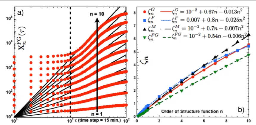
X_nFG( )t for all ordersn(ﬁgure4(a))could potentially arise from one of two very different mechanisms. If a day-Figure 4.(a)Log–log scale: cross-structure functionsXnFG( )t versusτ(solid red circles)exhibit no scaling at early timest10,

with scaling restored for10< <t 40. Solid black lines are power-lawﬁts to data within the scaling regime.(b)Scaling exponentz_nX versus the order of structure functionnfor generated G(solid red circles), forecast F(solid blue squares)and modiﬁed forecast M

(solid black triangles)structure functions, and cross-structure functions FG(solid green inverted triangles), and their respective second-order polynomialﬁts: solid red line for_z_nG_{, small dashed blue line for}

n

F

[image:8.595.120.550.62.273.2]

(9)

ahead forecast is regularly corrected at short timescales, one expects it will cause short timescale discontinuities in the forecast signal. Owing to these discontinuities, one cannot expectS_nF( )t 0ast0, especially for higher order structure functions(largen). EIRGRID generates a day-ahead forecast every calendar day at 00:00 Irish Standard Time(IST)for the next 24 h[30,31]. A time derivative of the raw(non-detrended)forecast time series p t

t F( ) ¶

¶ shows discontinuities only at 24 h intervals(00:00 IST of every calendar day). No short time discontinuities(up to within the sampling interval)were observed. One therefore infers either that EIRGRID does not employ short time corrections or that any such corrections do not exhibit discontinuities in the signal. Consequently, we conclude that short timescale discontinuities make no contribution to higher order structure functions. We, therefore, trace the absence of scaling fort10time steps to the second possibility. It must arise from the temporal resolution limitations of the EIRGRID models, including the fact that the boundary conditions for the regional model are only updated every six hours, hence our qualiﬁcation of this error as a timescale erroret.

5. Discussion

Having established the various structure functions, we now consider the behavior of their scaling exponentsz_nX (XºGfor generated, F for forecast and FG for the cross-structure function). Figure4(b)plots z_nX versus the orderntogether with their polynomialﬁts to the quadratic order._z_nG₌10-2₊0.67n_-0.013n2 _{scales almost} linearly(mono-fractal)with a small, but measurable, quadratic deviation towards multi-fractal behavior. The exponent_z_nF₌0.007₊0.8n_-0.025n2_{exhibits a slightly more pronounced quadratic deviation}₍_{multi-fractal} behavior)relative toz_nG. On the other hand,_zFG_n ₌10-2₊0.54n_-0.006n2 _{scales almost linearly with}_n_, implying mono-fractal scaling.

We now consider the measurement error for the aforementioned scalings. First, given that all detrending protocols suffer from the ad hoc choice of a detrending timescale, we tested the scalings for dependence on the detrending procedure by varying the number of maximal amplitudes. Ignoring the condition for maximal cross-correlation betweenpg(t)and pf(t), the number of maximal amplitudes contributing to the trends was varied. The scalings were invariant up to the inclusion of 15 maximal amplitudes into the trend, beyond which coefﬁcients for the polynomialﬁts started varying in the second decimal place.

[image:9.595.120.553.62.272.2]

Contrary to normal practice[19], we did not explicitly detrend the diurnal oscillation frequency as it was found not to be relevant for our analysis. First, we focused onﬂuctuations for timescales less than 24 h. In particular, we observed self-similar scaling in structure functions up to 10 h(t=40time steps). Since our analysis cannot apply beyond this timescale, diurnal oscillations do not enter into our analysis. Second, whereas diurnal peaks are present in the autocorrelation function(ﬁgure2(b))for the instantaneous forecast error (CD( )t ), we did not calculate structure functions for instantaneous forecast error(PD(t)). Diurnal modes are barely discernible for the autocorrelation functions of generated(CG( )t )and forecast power(CF( )t )whose

Figure 5.(a)Log-linear scale:g_optversus order of structure function shows no improvement forn<4but shows better agreement forn4with an abrupt change observed ing_optatn=4.(b)Log–log scale: structure functionsSnM( )t versusτ(solid red circles)

for the modiﬁed forecast time series show considerable improvement over their counterpartsSnF( )t inﬁgure3(b).

7

(10)

structure functions we do study. Finally, as stated earlier, our detrending protocol revealed that diurnal oscillations in the forecast and generated power are less signiﬁcant than other(much slower)processes. Having ascertained the robustness of our choice for theﬁve maximal amplitudes at which the cross-correlation peaks, we focused on a second source of scaling measurement error, namely statistical variability. Since the scalings are analyzed up tot =100data points, the detrended time series were split into eight independent windows(each with 21 912 data points), and the structure functions were recomputed for each window. The variation in the log derivative _n d S

d

X log

log

nX

(

( ( ))

)

( )

z = _tt for the eight independent measurements was taken as the possible scatter in the scaling estimation, thereby providing a conﬁdence interval for the polynomial

ﬁts. The scatter was found to bez_nX0.01in both the measured value of_z_nX_{and the corresponding polynomial}

fits(for each of the polynomial coefficients)for each of the eight independent datasets, revealing that the polynomialfits were meaningful only to the linear order forz_nGandz_nFG. The quadratic-order polynomial coefficient for_z_nF_{, despite being larger than the scatter of}__±_{0.01, is not useful owing to the fact that the} corresponding quadratic terms forz_nGandz_nFGare smaller than the scatter magnitude.

Despite qualitatively observing a quadratic deviation forz_nXinfigure4(b), our inability to ascribe significance to it arises from the fact that the multi-fractal component(deviation from linear scaling)of the scalings is minuscule. This is significant in light of several studies that have demonstrated multi-fractal scaling for wind powerfluctuations at the turbine[2,4]and farm scales[42]. Turbulence theory traces the source of multi-fractal behavior to intermittentfluctuations that can arise from two sources in the atmospheric context. Thefirst, known as internal intermittency, occurs at the small scales of turbulentflow. These intermittentfluctuations would be naturally reflected in the power generated at the turbine and farm scales. However, when adding together power generated by geographically distant wind farms, internal intermittency should smooth out[7]

since it is a small-scale effect and cannot extend across geographically distributed wind farms. Furthermore, the sampling interval(15 min)for EIRGRID data is not expected to resolve any effects that may arise from internal intermittency, which occur at much shorter timescales(high frequencies).

The second source of intermittency, known as external intermittency, occurs at the edge of any free-stream [43]and arises in the atmospheric context due to coupling between the atmospheric boundary layer turbulence and a co-moving weather system[28]. External intermittency, which can be experienced in the form of wind gusts, is of greater relevance in the present analysis as it can both correlate distributed farms through the weather system and occur at timescales longer than the 15 min sampling interval for the EIRGRID data. The nearly fractal scaling ofz_nGinforms us that both internal and external intermittency are being smoothed to the point of rendering grid-level powerﬂuctuations almost mono-fractal.

The self-similar scaling ofSnG( )t over several hours does strongly point to the influence of large-scale turbulent structures on powerfluctuations at the grid level. The 20 h characteristic decorrelation time(tG)for generated power infigure2(c), if taken as the large eddy turnover time of atmospheric turbulence, also lends credence to such an argument. Finally, independent proof in support of this argument also comes from

Katzensteinet al[7]who show that an individual wind farm exhibits f-5 3₍_f_{being the frequency}₎_{scaling for the} wind power spectrum(equivalent to_t2 3_{scaling of the second-order structure function in the time domain}₎_. However, as wind power from various farms is summed, the spectrum steepens(please seefigure 3 in[7]). Such spectral steepening can be clearly attributed to the smoothing of high frequency(short timescale)fluctuations corresponding to small eddies. But the low frequency(long timescale)fluctuations corresponding to large-scale eddies lose no power spectral density, clearly indicating the influence of large-scale turbulent structures on wind power. These large eddies extend across great geographic distances to couple distributed wind farms. No longer independent of each other, theirfluctuations become correlated, and thus cannot smooth out when summed at the electrical grid. This spatial coupling of wind farms via atmospheric turbulence manifests itself through correlatedfluctuations in the aggregate wind power feeding the electrical grid.

Wefinally consider the forecast error due to the scaling mismatch. We define the scaling error as ezºz_nF-z_nG. Under this definition, if the time series for forecast and generated power were identical, then S_nG( )t ºS_nF( )t , implyingz_nGºzF_n, and thereforeez=0. Another typical case arises if forecast models fail

completely, resulting in aﬂat time series with noﬂuctuations,z_nF=0, resulting in an errorez= -z_nG. Using

the polynomialﬁts forz_nX(seeﬁgure4(b))to the linear order, we obtainez=

n n n

7 10 3 0.8 10 2 0.67 0.003 0.13

( ´ - + )-( - + )= - + . This can be cross-validated against the difference_zG_n _-_zFG_n ₌₍10-2₊0.67n₎_-₍10-2₊0.54n₎₌0.13n_{. Since} ₀

n X

z  asn0, the 0th order term falling within the scatter may be taken to be zero. Both estimates of error are identical to the linear order(ez=0.13n).

(11)

forecast that is based on the original forecast, convoluted with an exponentially decaying memory kernel derived

from the generated power time series. The modiﬁed forecast power is given byP t P e d

t

t M

0 F

( )₌

ò

( )_t -g(-t) _t_. This modiﬁed forecast imposes a short-term correlation on the original forecast; therefore, it is expected to better capture the temporally correlatedﬂuctuations of the generated power.

The memory duration(1 g)was chosen so as to minimize the relative difference between the structure functions of the generated and forecast power. As expected(as shown earlier, the low order structure functions of the generated and forecast power are very similar), we found that the optimalγvaries with the order of the structure function. Forn<4, the memory-modiﬁed forecast shows no improvement in the agreement between Sn

G and Sn

F

. Forn4, the modified forecast exhibits better agreement with the structure functions of the generated power as shown infigure5(b). The optimalγ(g_opt)was found to beg₄»1.06andg₁₀»0.37, as shown infigure5(a), plotted in log-linear scale to show the variation ing_opt forn4. The simple scheme, suggested here, not only tries to rectify the timescale erroret, but also attempts to statistically align the temporal correlations by improving the scaling errorez.

As is apparent fromfigure5(b), the structure functions(SnM( )t º á D∣ PM( )∣t nñ)for modified forecast time series are substantially improved over their unmodified counterpart(figure3(b)). First, scalings are restored at high frequencies(t10), thus rendering the timescale error irrelevant. More importantly, the scaling itself is improved as is evident fromfigure4(b), revealing_z_nM₌0.01₊0.7n_-0.007n2_{. To the linear order, the} scaling errorez=z_nM-z_nG=0.7n-0.67n=0.03n, a considerable improvement over the original forecast time series. Being computationally inexpensive, and given that spinning and non-spinning reserves must act within 10 min of failure[44], with replacement reserves acting within 20–60 min, there are tangible benefits to incorporating such a memory kernel into models to monitor instabilities in real-time. Furthermore, it might be possible to improve the forecast models using different parameterizations of the regional climate models or weather models, or other stochastic approaches such as Markov-chain-based prediction methods[45]. It is important to note that the improvement in the prediction does not come at the expense of an increase in the error. We verified that for the values ofγ(in the memory kernel)that we used, the root mean squared error (rmse= P t P t

N t N 1

1( F( ) G( ))2

S= - )and the cross-correlation between the modiﬁed forecast and the generated power were within 1% of those of the original forecast.

6. Summary

In summary, wind power exhibits significant temporal correlations even at the grid level, wherefluctuations are expected to average out[5]as power is fed from geographically distributed wind farms. Previous studies have shown that the temporal correlations of the wind are essential to studying wind-generated large-scale ocean currents[46]; a similar appreciation of large-scale correlations in atmospheric turbulence within the context of wind power is called for. Fluctuations, albeit posing a problem to system operators, possess a statistical structure through temporal correlations, which could be exploited to quantitatively analyze the error in forecast models. The technique proposed here is only limited by the sampling rate of the time series. Beyond potentially serving as a standard for quantifying wind-power forecast accuracy, it could have applications for any renewable energy source with temporally correlatedfluctuations possessing a statistical structure.

Acknowledgments

MT and MMB were supported by the Collective Interactions Unit at the Okinawa Institute of Science and Technology Graduate University. CPC was hosted by the Collective Interactions Unit at the Okinawa Institute of Science and Technology Graduate University while performing this work. GB was supported through the European Union Seventh Framework Programme(FP7/2007-2013)under grant number 293825. The authors gratefully acknowledge EIRGRID for permission to use their data.

References

[1]MacKay D J C 2009Sustainable Energy—Without the Hot Air(Cambridge: UIT Cambridge)

[2]Milan P, Wächter M and Peinke J 2013Phys. Rev. Lett.110138701

[3]Apt J 2007J. Power Sources169369

[4]Calif R, Schmitt F G and Huang Y 2014Geophys. Res. Abstr.1615443

[5]Wiser R, Yang Z, Hand M, Hohmeyer O, Inﬁeld D, Jensen P H, Nikolaev V, O’Malley M, Sinden G and Zervos A 2011 Wind energy IPCC Special Report on Renewable Energy Sources and Climate Change Mitigation(Cambridge: Cambridge University Press)

[6]Jacobson M Z and Delucchi M A 2009Sci. Am.30158

[7]Katzenstein W, Fertig E and Apt J 2010Energy Policy384400

9

(12)

[8_]http:_//eirgrid.com_/operations_/systemperformancedata_/windgeneration_/

[9_]Irish Wind Energy Association₍http:_//iwea.com_/faqs₎

[10]Muzy J F, Baïle R and Poggi P 2010Phys. Rev.E81056308

[11]Lovejoy S, Schertzer D and Stanway J D 2001Phys. Rev. Lett.865200

[12]Lueken C, Cohen G E and Apt J 2012Environ. Sci. Technol.469761

[13]Katzenstein W and Apt J 2012Energy Policy51233

[14]Matos M A and Bessa R J 2011IEEE Trans. Power Syst.26594

[15]Tande J O G 2000Appl. Energy65395

[16]Albadi M H and El-Saadany E F 2010Electr. Power Syst. Res.80627

[17]Fabbri A, Gomez San Roman T, Abbad R and Quezada V H M 2005IEEE Trans. Power Syst.201440

[18]Parsons B P, Milligan M, Zavadil B, Brooks D, Kirby B, Dragoon K and Caldwell J 2004Wind Energy787

[19]Costa A, Crespo A, Navarro J, Lizcano G, Madsen H and Feitosa E 2008Renew. Sustainable Energy Rev.121725

[20]Doherty R and O’Malley M 2005IEEE Trans. Power Syst.20587

[21]Bludszuweit H, Dominguez-Navarro J A and Llombart A 2008IEEE Trans. Power Syst.23983

[22]Hodge B M and Milligan M 2011NREL Report No.: NREL/CP-5500-50614

[23]Hodge B M, Ela E G and Milligan M 2012Wind Eng.23509

[24]Hodge B Met al2012 Wind power forecasting error distributions: an international comparisonTech. RepNational Renewable Energy Laboratory

[25_]Wu J, Zhang B, Li Z, Chen Y and Miao X 2014Electr. Power Energy Syst.55100

[26_]Madsen H, Pinson P, Kariniotakis G, Nielsen H A and Nielsen T S 2009Wind Eng.29475

[27]Lange M 2005J. Sol. Energy Eng.127177

[28]Katul G G and Chu C R 1994Phys. Fluids62480

[29]Weber C 2010Energy Policy383155

[30]Lang S C, Möhrlen J, Jørgensen B, Gallachóir O and McKeogh E 2006 Forecasting total wind power generation on the republic of ireland grid with a multi-scheme ensemble prediction systemProc. Global Wind Energy Conf. GWEC Adelaide

[31]Lang S and McKeogh E 2009Wind Eng.33433–48

[32]German TSO Intraday Market:www.epexspot.com/en/product-info/Intraday/germany

[33]Kolmogorov A N 1941Dokl. Akad. Nauk SSSR3216

[34]Frisch U 1995Turbulence: The Legacy of A. N. Kolmogorov(Cambridge: Cambridge University Press)

[35]Bandi M M, Goldburg W I, Cressman J R and Pumir A 2006Phys. Rev.E73026308

[36]Samorodnitsky G and Taqqu M S 1994Stable Non-Gaussian Random Processes(New York: Chapman and Hill)

[37]Anselmet F, Gagne Y, Hopﬁnger E J and Antonia R A 1984J. Fluid Mech.14063

[38]Anselmet F and Antonia R A 1984J. Fluid Mech.14063

[39]Mandelbrot B and Hudson R L 2004The Misbehaviour of Markets: A Fractal View of Financial Turbulence(New York: Basic Books)

[40]Chen S Y, Dhruva B, Kurien S, Sreenivasan K R and Taylor M A 2005J. Fluid Mech.533183

[41_]Larkin J, Bandi M M, Pumir A and Goldburg W I 2009Phys. Rev.E80066301

[42_]Calif R, Schmitt R and Huang Y 2013PhysicaA3924106

[43_]Kuznetsov V R, Praskovsky A A and Sabelnikov V A 1992J. Fluid Mech.243595

[44_]Billinton R and Allan R 1996Reliability Evaluation of Power Systems₍New York: Plenum₎

[45]Pesch T, Schröders S, Allelein H J and Hake J F 2015New J. Phys.17055011

[46]Bel G and Ashkenazy Y 2013New J. Phys.15053024