ACE, ARIMA



Abstract—Globally there is a spur in demand of natural gas

and business entities are interested to realize natural gas price forecast. The forecast is likely to suffice to different objectives to producers, suppliers, traders and bankers engaged in natural gas exploration, production, transportation and trading as well as end users engaged in utilization of natural gas. For the supplier the objective is to meet the demand with profit and for the trader it is for doing business. Researchers have invoked different methodologies to forecast natural gas price. It was intended to develop a model to forecast natural gas price in terms of specific parameters which may have relationship with natural gas price by applying Time Series as well as nonparametric regression invoking Alternating Conditional Estimation (ACE). Discernible predictor variables that may elucidate statistically important amount of the inconsistencies in the response variable have been recognized and the correlation between variables has been established. Statistical tests and techniques viz. unit root and ADF tests, and ARIMA have been applied. Present work is an attempt to demonstrate these models pertaining to natural gas pricing.

Index Terms— Natural Gas Price, Crude Oil, Time Series, ACE, ARIMA

I. INTRODUCTION

ATURAL gas, an important ingredient in the global energy-market is poised to play an increasingly important role in meeting global energy demand. Due to global abundance, diversity of usage, burning efficiency and environmental considerations it is the preferred fuel of modern civilization. Nation’s desire to secure gas supply is poised to set off radical interdependencies and geopolitical alignments resulting in spur in the development of infrastructure for trading of gas across the globe and concomitant escalation in natural gas trade across international borders leading to far-reaching impact on the world energy trade. Natural gas markets were earlier considered to be isolated, with prices varying from country to country. But, with advent of LNG and cross-country gas pipelines the natural gas trade has taken global dimension. As the use and trade of natural gas continue to grow, it is expected that pricing mechanisms will continue to evolve, facilitating international trade and paving the way for a global natural gas market. Thus, a realistic estimate of natural gas price is prerequisite for due diligence of projects and trade. Very often governments plays significant role in devising a mechanism to keep the end user price of natural gas stable.

Manuscript received March 23, 2012; revised April 10, 2012.

Prerna Mishra is B. Eng. Third Year student at the Nanyang Technological University, 50 Nanyang Avenue, Republic of Singapore, Cell phone: +65 84535692; ( e-mail: [email protected]).

Natural gas, like crude oil, is explored, produced, transported and delivered to end user. The end user price of crude oil and natural gas includes several components. Carrying natural gas from the well head to end user is capital intensive. The consideration of well-head price, follows the fundamentals of “cost plus basis” which is the sum of costs in respect of exploration and production, storage, transportation, distribution, profit and taxes. It in essence leads to “Net Back Price” (NBP) which is explained by the following equation.

Net Back Price = End user delivery price of alternate fuel to the customer (say crude oil) - Transportation cost from storage to market – Storage cost – Taxes.

If the transportation, storage and delivery cost for crude oil and natural gas are identical then the NBP will be equal to end user or delivered price. However in practice this is not the case. Except the exploration and production costs (which governs the well head price) all other cost elements are different for crude oil and natural gas. The exploration cost of crude oil and natural gas is comparable but the production, transportation, and marketing costs varies considerably. Therefore, for modeling purpose, it is proposed to consider the US Crude Oil first purchase price [16] and US Natural Gas well head price [17].

II. LITERATUREREVIEW

Doris (1999) [1] provided a methodology for prediction of short-term natural gas prices using econometrics and neural network. According to the author, developing a quantitative model to predict natural gas price based on market information holds key to price risk management owing to volatile natural gas spot prices, and because prevalent practice in price prediction focuses on long term equilibrium price forecast with no consideration for day-to-day volatile behaviour of spot prices. This model may hold well for long-term contracts, but not for day-to-day prediction of spot price, which is provided by the econometric and neural network model developed by Doris (1999). Solomon (2001) [2] has critically analyzed the impact of oil and natural gas prices on oil industry activities invoking linear regression analysis and have made an attempt to forecast future oil and gas prices. Zamani (2004) [3] has proposed an econometrics forecasting model of short term oil spot prices. Pindyck (1994) [4] has investigated the relationship between stocks and prices in the short run for copper, lumber and heating oil. Stephane et al (2003) [5] has made an attempt to forecast real oil price. Agbon (2003) [6] has recognized the chaotic behaviour of historical time

Forecasting Natural Gas Price - Time Series and

Nonparametric

Approach

Prerna Mishra

series oil and gas spot prices and suggests the use of nonlinear models for prediction. Jablonowski et al (2007) [7] proposed a decision-analytic model to value crude oil price forecast. Ogwo (2007) [8] has proposed an equitable gas pricing model. The literature review offered various methodologies put forward to forecast natural gas price. Each method has advantage and limitations. In order to overcome such limitations, it is envisaged to invoke econometrics and nonparametric technique to develop model to estimate natural gas. Nonparametric techniques viz. Alternating Conditional Expectation (ACE) [9] has been widely applied to identify the relationship between dependent and independent variables. Briemann et al (1985) [9] provide detail account of estimating optimal transform for multiple regression and correlation. Duolao et al (2004) [10] and Guoping et al (1997) [11, 12] discuss in detail about ACE algorithm. Gujarati (2007) [13] and Ramanathan (2002) [14] provide description of Time Series Analysis. Jon et al (2011) [15] provide application of ACE in modeling parameters. It has been observed that no previous research has focused on development of models to estimate natural gas price using time series analysis to find relationship between crude oil and natural gas prices. It is considered to model the time series data of crude oil and gold invoking time series and nonparametric techniques to estimate natural gas price. The models may find practical application in natural gas price estimation.

III. FACTORS OF CONSIDERATION

Historical data (Fig1) depict that in general the US Crude Oil First Purchase Price [16], US Natural Gas Well Head Price [17], and Gold Price [18] bear resemblance. Events in the world history have impacted crude oil price as depicted by spikes in the figure. The similarity in price behavior suggests that the factors which impacted crude oil price have impacted natural gas price as well. Indeed natural gas is the product of same natural system as crude oil, is explored and produced by similar mechanism, has identical utilization. Having agreed on the similarity of historical price behavior of the two products, it is intended to establish a correlation between the prices of these products in

historical past and find a way to predict the price of natural gas in terms of price of crude oil. Furthermore, it is generally agreed that gold is the most commonly traded commodity globally and its price has governed the global market and national currencies. Therefore, in order to derive a relationship between crude oil price and natural gas price, the price of gold has been brought into play and attempt has been made to establish the relationship between prices of these commodities by invoking Alternating Conditional Estimation (ACE) [9].

IV. MODELING PARAMETERS

The US Natural Gas Well Head Price [17] has been considered as dependent (Response) variable where as the US Crude Oil First Purchase Price [16] and Gold Average price [18] have been considered as independent (Predictor) variables. Time Series data (monthly data) for the period January 1976 to September 2011 constitute the input parameters for modeling. The abbreviations - US Crude Oil First Purchase Price - USCOFPP (USD/Barrel), US Natural Gas Well Head Price- USNGWHP (USD/TCF), and Gold Average Price - GP (USD/Gram) have been used. USD and TCF are acronym for United States Dollar and Trillion Cubic Feet respectively. Barrel is the unit of volume in which crude oil is measured and one US barrel is 42 US gallons.

V. MODELING METHODOLOGY

Gathering information from the past constitutes the first step in forecasting. Records of historical statistical data sets of variables recorded at successive periodic intervals (monthly) constitute the first step in forecasting. Thus in essence statistical data which will be dealt with are observed or recorded at successive (monthly) intervals also known as time series where each independent data series representing variables are related to time. It is observed that in general the natural gas price has increased over the years, but, there are some episodic fluctuations as well where there is a “sharp deviation” from the general trend. These sharp fluctuations in natural gas price may be explained by several exogenous or endogenous factors. Endogenous factors are those which arise from some interrelated activities within the petroleum industry itself. Exogenous factors include issues like seasonality in demand and supply arising due to surge in demand during winter or decline during summer, natural calamities disrupting supply chain, geopolitical issues etc. It is really difficult to account for the relative degree influence of influence of each of the factors affecting natural gas price at any particular moment. However some major cause may be assigned to observed “sharp deviation”. It is not the purpose of this paper to cite these impacting parameters which may be due to changes that have occurred as a result of following

- general tendency of the data to increase or decrease, known as “secular movements,

- weather condition, also known as “seasonality of price fluctuations”,

- economic fluctuations (benchmarked with respect to Fig. 1 Historical US Crude Oil First Purchase Price (USD/Barrel), Natural

changes in standard currency viz. US Dollar or Euro price), also known as “cyclical variations”,

- natural calamities, geopolitical issues, also known as “irregular or erratic variations”.

According to Ramanathan (2002) [14], in time series any dependent variable (Y) is modeled as a function of a trend component (T), a seasonal component (S) and a random (or stochastic) component (U), described by equation Y = T*S*U; where * represents an arithmetic operator and S is due to regularly occurring seasonal phenomenon. Thus, while selecting requisite model due consideration has been given to impact due to the elements leading to seasonality in price behavior as evidenced in time series (Fig 2).

Most commonly, the natural gas price can be estimated from

different parameters impacting it by using either empirical relationship or some form of regression. Regression has been proposed as a versatile solution to the problem of estimation. Conventional statistical regression has generally been done parametrically using multiple linear or nonlinear models that require a priori assumptions regarding functional forms. It is proposed that methods employing econometrics and non parametric regression to derive functional relationship between natural gas price and crude oil price or gold price be used and an attempt has been made to apply the Time Series Model and Alternating Conditional Expectation (ACE) algorithm for estimation of the natural gas price from crude oil price or gold price.

VI. DESIGN OF EXPERIMENT

The experiment has been designed on the premise that it may be advantageous to work out a model integrating all impacting parameters viz. crude oil price and gold price. The relationship may be deduced by applying different mathematical techniques parametric or non parametric regression. In parametric regression, a model is fitted to data by assuming a functional relationship. However, it is always not possible to identify the underlying functional relationship between response and predictor variables. Nonparametric regression technique offer much more flexible data analysis tools for exploring the underlying relationships between response and predictor variables.

The historical crude oil and natural gas price data are non-linear in nature. According to Agbon (2003) [6], the

non-linear nature of spot prices make prediction very difficult. Linear models have been proposed to forecast crude oil and natural gas prices. These models are based on premise that prices increase monotonously and some elements of price and demand elasticity have been introduced into the model [6]. It is hypothesized that in this problem the considered predictor variables i.e. crude oil and gold prices do not hold linear relationship with response variable (i.e. natural gas price). Thus, it is intended to model these parameters by invoking nonparametric regression techniques such as ACE. The rational behind preferring nonparametric to parametric lies in the fact that in parametric regression a model is fitted to data by assuming a functional relationship. But, it may not be possible to recognize the underlying functional relationship between dependent (response) and multiple independent (predictors). Nonparametric regression explores such relationship without a priori knowledge of the dependencies and the functional form is derived from data.

An attempt has been made by invoking ACE and ARIMA to develop models and see the agreement or disagreement of forecast (in-sample forecasts of Ramanathan, 2002) [14] with observed values of dependent parameter. It is implicit that the extent of conformity between in-sample forecast with observed values of dependent variable may provide a clue to the robustness of model for future time periods (out-of-sample ex-ante forecasts of Ramanathan, 2002). The models have been evaluated or compared by taking in to account the Mean Squared Error (MSE), Akaike information Criteria (AIC) etc.

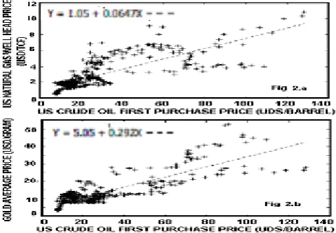
VI. A. Correlation and Regression Analysis

The Pearson correlation coefficient with 2-tailed test of significance between USCOFPP and USNGWHP is 0.78 and between USCOFPP and GP is 0.84. It suggests perfect positive correlation coefficient depicting high degree linear relationship. The simple linear regression model between USCOFPP and USNGWHP and USCOFPP and GP lead to R2= 0.6068 and 0.5409 respectively (Fig 3). Multiple linear regression of USNGWHP and USCOFPP and GP has

Square of 0.73.

Since, heteroskedasticity may be an expected concern, therefore, heteroskedasticity corrected model (Table-1 to 3 and Fig.4) for USNGWHP as dependent variable has been attempted using Gretl [14].

Table 1. Heteroskedasticity-corrected Model

Coeff. Std. Error t-ratio p-value USCOFPP 0.09365 0.0041937 22.33 <0.00001

GP 0.01786 0.0077783 2.297 0.02212

Table 2 Heteroskedasticity-corrected Model (Statistics based on the weighted data) Sum squared

resid

1028.47 S.E. of regression

1.551967 R-squared 0.58573 Adj. R-squared 0.584768 F(2, 427) 301.87 P-value(F) 1.94e-82

Log-likelihood

-796.27 Akaike criterion 1596.556 Schwarz

criterion

1604.67 Hannan-Quinn 1599.763

rho 0.96615 Durbin-Watson 0.098623

Table 3 Heteroskedasticity-corrected Model (Statistics based on the original data) Mean

dependent var

2.89069 S.D. dependent var

1.917536 Sum squared

resid

934.709 S.E. of regression

1.479532

The forecast (figure 4) has following pertaining to the evaluation of forecast - Mean Error = -0.016454, Mean Squared Error = 2.1788, Root Mean Squared Error = 1.4761, Mean Absolute Error = 0.89641, Mean Percentage Error= -3.2296, Mean Absolute Percentage Error= 27.612.

VI.B Time Series Analysis

Time Series represents a set of observations taken at equal intervals, viz. the values Y1, Y2, …..Yn of a variable Y at a time t1,t2…..tn. Analyzing time series may be of help in understanding past behavior and thus predict within limits the future behavior by realizing the pattern of regularities of occurrences of any feature over time. Comparison of different time series may lead to important logical

derivations by relating variables in each series to their past values. It is intended to use time series data in the analysis. Time series data under consideration are the data in respect of monthly price of USCOFPP, USNGWHP and GP. These data sets represent stochastic process (i.e. collection of random variable ordered in time). The price of these products could have been any number, depending on the complex interplay of domestic and global economic and political environment. Accordingly, the price at any particular time is a particular realization of all such possibilities.

An empirical work based on time series data requires that the underlying time series is stationary. Thus, it requires finding out whether that data is stationary or not. Another requirement is to check for autocorrelation due to non-stationarity. It is also important to find out whether the regression relationship between variables is spurious, because very often the spurious regression results due to non-stationary time series. It is needed to know now if a meaningful relationship exists between variables. Because, very often very high R2 value is obtained even though there exists no meaningful relationship. It is also important to find out whether the time series exhibit Random Walk Phenomena, because, then the forecasting will be futile. Moreover, it is prudent to know if such forecasting is valid if the time series under consideration is non-stationary. A time series is said to be stationary if it’s mean, variance and auto-covariance remains the same at any point of time. The process that generates the stationary series is time-invariant (Ramanathan, 2002) [14]. If a time series is non-stationary, its behavior can be studied for the time period under consideration and no generalization can be made for the entire period. For the purpose of forecasting non-stationary time series holds no significance.

VI.B.i Test of Stationarity of Time Series

In order to test for stationarity, Augmented Dickey Fuller (ADF) Test is conducted for the time series data. It is supposed that the more negative the Dickey Fuller Test statistic value and lesser the p value, there is more chance for the series to be stationary. The output of ADF test (Table 4) suggests that the natural gas well head price time series is stationary, but, the time series of crude oil price exhibits random walk process and non stationarity. The time series of gold price exhibits non stationary behavior. ADF test of difference of log prices of crude oil and natural gas, and crude oil and gold provide the p value as 0.702209 and 0.176501 respectively, which indicate that the series are not mean reverting.

Table 4 Output of ADF Test

Crude oil Natural Gas Gold Dickey Fuller

Test Statistic

-1.68366 -3.47299 2.48024

p-value 0.711171 0.045213 0.99

series to derive significant statistics or else prefer a technique which takes care of stationarity issue, because it is meaningless to exercise regression models fitted to nonstationary data.

VI.C ARIMA Model

Auto Regressive Integrated Moving Average (ARIMA) model has been used. ARMA models represent combination of Auto Regressive (AR) and Moving Average (MA) models. AR (p) and MA (q) represent models p and q order respectively. By differencing d times any nonstationary series can be converted to stationary form and the process that generates the stationary series is called auto regressive integrated moving average, and the model is called ARIMA (p,d,q) model. It provides solution for non stationary time series and can transform it to a stationary time series by differencing. Simultaneous equation models very much in vogue during 1970’s may not be relevant for economic forecasting due to their limitations and “Lucas Critique” which championed that the response parameters are not invariant/ insensitive to policy changes (Gujarati, 2007) [13] and thus has not been used in this work. Indeed, policy changes may substantially impact the price behavior of the time series data that has been worked upon.

VI.C.i ARIMA Model (Hessian)

The ARIMA (1, 2, 1) model using Standard errors based on Hessian (Table 5, 6 and Fig 5) provide reasonable forecast of dependent variable USNGWHP.

Table 5 ARIMA Model (Standard errors based on Hessian)

Coeff. Std. Error z p-value

GP 0.02731 0.023024 1.1865 0.23544

USCOFPP 0.03515 0.006604 5.3234 <0.00001 Table 6 ARIMA Model (Standard errors based on Hessian)

Mean

dependent var

2.890699 S.D. dependent var

1.917536 Mean of

innovations

0.002629 S.D. of innovations

0.418881

Log-likelihood

-236.6259 Akaike criterion

485.2517

Schwarz criterion

509.6205 Hannan-Quinn 494.8751

VI.C.ii Cochrane-Orcutt Model

The ARIMA (1,2,1) model using Standard errors based on Cochrane-Orcutt (Table 7,8 and Fig. 6) provide reasonable forecast of dependent variable USNGWHP. Table 7 ARIMA Model (Cochrane-Orcutt)

Coeff. Std.

Error

t-ratio p-value GP 0.046625 0.022414 2.0802 0.03811 USCOFPP 0.034994 0.006405 5.4635 <0.00001 Table 8 ARIMA Model (Cochrane-Orcutt) Statistics based on the rho-differenced data

Mean

dependent var

2.896192 S.D. dependent var

1.916398 Sum squared

resid

75.91233 S.E. of regression

0.422135 R-squared 0.952007 Adjusted

R-squared

0.951894 F(2, 426) 2.31038 P-value(F) 6.10e-10

rho 0.009027

Durbin-Watson

1.978968

VI.C.iii Prais-Winsten Model

The ARIMA (1, 2, 1) model using Standard errors based on Prais - Winsten (Table 9, 10and Figure 7) provide reasonable forecast of dependent variable.

Table 9. ARIMA Model (Prais-Winsten)

Coeff. Std. Error t-ratio p-value

GP 0.04665 0.022371 2.0854 0.03763

USCOFPP 0.03499 0.006396 5.4712 <0.00001 Table 10. ARIMA Model (Prais-Winsten) Statistics based on the rho-differenced data

Mean

dependent var

2.89069 S.D.

dependent var

1.917536 Sum squared

resid

75.9125 S.E. of regression

0.421641 R-squared 0.95217 Adjusted

R-squared

0.952062 Fig. 5 USNGWHP – Observed versus Forecast (Hessian Model)

F(2, 427) 22.4049 P-value(F) 5.59e-10

rho .009038

Durbin-Watson

1.978952

VI.C.iv Hildreth-Lu Model

The ARIMA (1, 2, 1) model using Standard errors based on Hildreth-Lu (Table 11,12 and Figure 8) provide reasonable forecast of dependent variable.

Table 11. ARIMA Model (Hildreth-Lu)

Coeff. Std.

Error

t-ratio p-value GP 0.046545 0.022440 2.0742 0.03866 USCOFPP 0.034973 0.006406 5.4595 <0.00001 Table 12 ARIMA Model (Hildreth-Lu)

Mean

dependent var

.896192 S.D. dependent var

1.916398 Sum squared

resid

5.91233 S.E. of regression

0.422135 R-squared 0.952007 Adjusted

R-squared

0.951894

F(2, 426) 2.22600 P-value(F) 6.58e-10 rho .008868 Durbin-Watson 1.979290

VI.C.v GARCH Model

The GARCH model using Standard errors based on

Hessian (Table 13, 14 and Figure 9) provide inferior forecast of dependent variable as compared to other ARIMA models.

Table 13 GARCH Model

Coeff. Std. Error z p-value

GP 0.05072 0.004850 10.456 <0.00001 USCOFPP 0.06995 0.001475 47.415 <0.00001 Table 14 GARCH Model

Mean

dependent var

2.890699 S.D.

dependent var

1.917536

Log-likelihood

-365.4702 Akaike criterion

742.9403

Schwarz criterion

767.3091 Hannan-Quinn

752.5637

Summarizing from above, it can be said that various models may be exercised to forecast US Natural Gas Well Head Price taking in to consideration the dependent variables. Each model provide with varying degree of certainty the forecast, and reasonable match has been observed between observed and forecasted values of dependent variable.

VI.C.vi. Non Parametric Regression – ACE Model

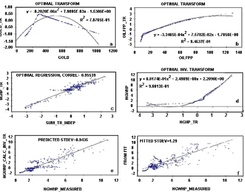
Alternating Conditional Expectation (ACE) method has been invoked which is based on non-parametric regression. In non-parametric regression a priori knowledge of the functional relationship between the dependent variable y and multiple independent variables x1, x2,…. xn is not required. In fact, one of the main results of such regression is determination of the actual form of this relationship. ACE generates an optimal correlation between a dependent variable and multiple independent variables through non-parametric transformations of the dependent and independent variables. Non-parametric implies that no functional form is assumed between the dependent and independent variables and the transformations are derived solely based on the data set [9, 10, 11, 12, and 18].

The Time Series data have been modeled by ACE to derive functional relationships between predictor variables to find response variable, the focus of this study. The ACE provides (figures 10 and transforms given in equations i, ii,

Fig 9. USNGWHP– Observed versus Forecast (GARCH Model) Fig. 7 USNGWHP – Observed versus Forecast (Prais-Winsten Model)

and iii) Predicted Std dev = 0.9435, Fitted Std dev = 1.29,

Optimal Regression Correlation = 0.95, and Optimal Inverse Trans. R2 = 0.96. The value of dependent variable i.e. Natural Gas Well Head Price (NGWHP) may be estimated from the transform in equation iii.

GP_Tr = -0.000008x2 + 0.007910x - 1.5306 - (i) USCOFPP_Tr= -0.000335x2 + 0.075702x - 1.7056 - (ii) NGWHP= 0.68174SumTr2 + 2.4909SumTr + 2.209 - (iii) Tr is an abbreviation for Transform and SumTr is sum of transform of independent variables GP and USCOFPP i.e. SumTr = GP_Tr + USCOFPP_Tr. The values of GP_Tr and USCOFPP_Tr may be obtained from the equations i and ii respectively.

The result of ACE provides a model characterizing numerical relationship between response and multiple predictor variables. The parameters considered in the model (US Crude oil first purchase price and Gold price) have been observed to have significant correlation with response variable (Natural Gas Well Head Price) as evidenced by strong regression correlation.

VII. ANALYSIS OF RESULTS

The estimate of US Natural Gas well head price (the dependent variable) have been attempted using values of independent variables viz. US Crude Oil first purchase price and Gold average price by applying time series and non parametric regression. Nonparametric regression methodology called Alternating Conditional Estimation (ACE) algorithm and Time series model using Autoregressive integrated moving average (ARIMA) has been used to derive functional relationship between the dependent (response) variable and multiple independent (predictor variables). All time series models except GARCH provide well-defined and comparable values of forecast against the observed values. The closeness in estimated and observed values corroborates that the estimated model is able to provide adequate fit to the data. However, the ARIMA (1, 2, 1) model using standard errors based on Hessian seems to outperform other time series models. The transform obtained by ACE has an optimal regression coefficient of 0.95 and the satisfactory fit is observed between measured and that derived from transform.

VIII. CONCLUSION

During the past decades the natural gas business has taken a truly global dimension. It calls for reasonable forecast of its price to mitigate price risk. Several methodologies have been proposed to forecast natural gas price. An approach may be to have the forecast in terms of price of associated product i.e. crude oil and globally traded merchandise viz. standard currency or gold. The simplest model may be to develop linear regression relationship. But, it may not be possible to find the degree of influence of various independent variables on the price of natural gas. It is reasonable to devise methodologies which take into cognizance the factors under consideration to derive natural gas price by employing techniques which avoid a priori underlying assumptions about relationship between the influencing factors, and the results thus derived honor the relationship for historical data sets of predictor and response variables. The solution to the problem is contingent upon numerical modeling of time series data sets. ARIMA and ACE offer technique for exploring the underlying relationships between dependent and independent variables. The result obtained by these techniques suggests that these may be used with reasonable degree of confidence. Nevertheless, it is obvious that although these techniques may provide estimate of natural gas price, it may be prudent to take into consideration factors which impact natural gas price on spatial and temporal basis and may jeopardize the predictions. Moreover, it should be realized that successes of these models depend on the quality and volume of the data.

REFERENCES

[1] Doris F. Reiter, “Prediction of short-term natural gas prices using econometric and neural network models,”, presented at SPE Hydrocarbon Economics and Evaluation Symposium, Dallas, Texas, March 21-23, 1999, pp. 1-10, SPE publication # 52960..

[2] Solomon O. I, Kunju M K, Omowunmi O I, “The responsiveness of global E&P industry to changes in Petroleum prices: Evidence from 1960-2000,” presented at SPE Hydrocarbon Economics and Evaluation Symposium, Dallas, Texas, April 2-3, 2001, pp 1-12. SPE publication # 68587.

[3] Zamani, “An econometrics forecasting model of short term oil spot prices,”6th IAEE European Conference, 2004, pp. 1–7.

[4] Pindyck, “Inventories and the short term dynamics of commodity prices,” Rand Journal of Economics, pp. 141–159, 25, 1, 1994.

[5] Stephane Dees, Sanchez, Marcelo, Karadeloglou, Pavlos, and Kaufmann, Robert K, “Modeling the world oil market: Assessment of a quarterly econometric model,” Energy Policy, Volume 35, Issue 1, pp 178-191, January 2007.

[6] Agbon I.S, and Araque J.C, “Predicting oil and gas spot prices using chaos Time Series Analysis and Fuzzy Neural Network model,”, presented at SPE Hydrocarbon Economics and Evaluation Symposium, Dallas, Texas, April 5-8, 2003, pp 1-8, SPE publication # 82014

[7] Jablonowski C and MacAskie R, “The value of oil and gas price forecasts,” presented at SPE Hydrocarbon Economics and Evaluation Symposium, Dallas, Texas, April 1-3, 2007, pp. 1-8, SPE Publication # 107570. [8] Ogwo O.U.J, “Equitable gas pricing model,” presented

at the 31st Nigeria Annual International Conference and Exhibition, Abuja, Nigeria, August 6-8, 2007, pp. 1-17, SPE Publication # 11897.

[9] Briemann, Leo. and Friedman, Jerome. H.,“ Estimating Optimal Transform for multiple Regression and correlation,” Journal of the American. Statistical Association, Vol. 80, No. 391 pp. 614-619, Sep., 1985. [10] Duolao, Wang, “Estimating optimal transformations

for multiple regression using the ACE Algorithm,”

Journal of Data Science 2, pp. 329-346, 2004.

[11] Guoping Xue, “Optimal Transformations for multiple regression: Application to permeability estimation from well logs,” SPE Formation Evaluation, pp 85-93, 1997.

[12] Guoping Xue, Datta-Gupta, A., Valkó, P. and Blasingame, T. A., “Optimal Transformations for Multiple Regression, Application to Permeability Estimation from Well Logs,” SPE Formation Evaluation, Vol. 12(2), pp 85-93, 1997.

[13] Gujarati, “Basic Econometrics,” Fourth Edition, The Tata McGraw-Hill Companies Publishing Company Ltd., 2007.

[14] Ramu Ramanathan, “Introductory Econometrics with Applications,” Fifth Edition, Thomson South-Western, 2002.

[15] Jon Quah and Prerna Mishra, “Application of Non Parametric Regression Network to model Risk Parameters for ranking countries to carry out business in water, electronics, education, pharmaceuticals, and infrastructure sectors (Published Conference Proceedings),” in Proceedings of the 2011 International Conference on Information & Knowledge engineering, July 18-21, Las Vegas, USA, Worldcomp’2011, USA, pp. 199-204.

[16] http://www.eia.gov/dnav/pet/hist/LeafHandler.ashx?n= PET&s=F000000__3&f=M, accessed on 20.12.2011. [17] Energy Information Administration,

http://tonto.eia.gov/dnav/ng/hist/n9190us3m.htm, Dec. 2011 (11/29/2011), accessed on 20.12.2011.