Study on Strain Gradient Sensing and Flexoelectric Micro/nano Structures.

ABSTRACT

HUANG, WENBIN. Study on Strain Gradient Sensing and Flexoelectric Micro/Nano Structures. (Under the direction of Dr. Xiaoning Jiang).

Flexoelectricity defines the electric polarization induced by mechanical strain gradient, or the mechanical strain generated under an electric field gradient. Compared with the more widely applied electromechanical coupling effect, piezoelectricity, flexoelectricity is free of the material symmetry limitation and exists in all dielectrics in principle. However, flexoelectricity has not attracted much of research interest until very recently, attributing to the experimental demonstration of large flexoelectricity in high permittivity ferroelectric materials.

To demonstrate the size independence of flexoelectricity in ferroelectric materials, we investigated the transverse flexoelectric coefficient in cantilever structures with the thicknesses ranging from millimeter to tens of micrometers. Consistence of the measurement results indicate that flexoelectric microstructures holds great potential for sensing/actuating applications due to the scale effect of the flexoelectricity. On the other hand, shear flexoelectric coefficient of ferroelectric ceramic was measured in the converse manner for the first time. These work lay the foundation of attaining the comprehensive flexoelectric tensors.

strain gradient sensor was further used to monitor the curvature of mechanical structures. The curvature sensor provides a sensitivity of 30.78 pCm in comparison with 32.48 pCm from theoretical prediction. In addition, the bending stiffness can be acquired from beam moment-curvature relationship that is derived from the moment-curvature sensor reading and is verified by Euler-Bernoulli beam theory. In addition, the strain gradient sensor was applied to read out the curvature alteration and the moment of stiffness of the structure, which lacks a sensitive approach by conventional fiber optic or strain gauge methods. Furthermore, the strain gradient sensor was employed to measure the opening mode stress intensify factor. The effect of constant stress component in precisely determining the stress intensity factor KI can be

eliminated by SGS assisted measurement, attributed to the nature of strain gradient. This helps to diminish the measurement error to less than 5%. Given the known intensity factor the crack, the strain gradient sensor could be used to monitor the crack initiation and propagation status.

Study on Strain Gradient Sensing and Flexoelectric Micro/Nano Structures

by Wenbin Huang

A dissertation submitted to the Graduate Faculty of North Carolina State University

in partial fulfillment of the requirements for the degree of

Doctor of Philosophy

Mechanical Engineering

Raleigh, North Carolina 2014

APPROVED BY:

_______________________________ ______________________________

Dr. Larry Silverberg Dr. Jacob Jones

________________________________ ________________________________

DEDICATION

BIOGRAPHY

Wenbin Huang was born on Oct 8, 1988 in China. He received his Bachelor of Science in Precision Machinery & Instrumentation from University of Science and Technology of China in 2010. In August 2010, he started his graduate study as a Ph. D. student in the Department of Mechanical & Aerospace Engineering, North Carolina State University. Currently, he is working as a Research Assistant at the Micro/Nano Engineering Laboratory directed by Dr. Xiaoning Jiang. Wenbin’s main research interests include flexoelectric strain gradient sensing and micro/nano devices study.

Journal Articles

1) Huang, W., L. Shu, S.R. Kwon, S. Zhang, F.G. Yuan, X. Jiang, “Fabrication and Measurement of A Flexoelectric Micro-pyramid Composite”, AIP Advances, (2014). (Submitted)

2) Kwon, S.R., W. Huang, L. Shu, F.G. Yuan, J.P. Maria, X. Jiang, “Flexoelectricity in Barium Strontium Titanate Thin Film”, Applied Physics Letters, 105(14), 142904 (2014).

3) Li, Y., L. Shu, W. Huang, X. Jiang, H. Wang, “Giant Flexoelectricity in Ba0.6Sr0.4TiO3/Ni0.8Zn0.2Fe2O4 Composite”, Applied Physics Letters, 116(14), 144105, (2014).

4) Shu, L., F. Li, W. Huang, X. Wei, X. Yao, X. Jiang, "Relationship between Direct and Converse Flexoelectric Coefficients", Journal of Applied Physics, (2014). (Accepted) 5) Huang, W., S. Yang, N. Zhang, F.G. Yuan, X. Jiang, "Direct measurement of opening

mode stress intensity factors using flexoelectric strain gradient sensors", Experimental Mechanics, (2014). (In press)

6) Huang, W., S.R. Kwon, S. Zhang, F.G. Yuan, X. Jiang, "A trapezoidal flexoelectric accelerometer", Journal of Intelligent Material Systems and Structures, 25(3), 271 (2014).

8) Jian, X., S. Li, W. Huang, Y. Cui, X. Jiang, "Electromechanical response of micromachined 1-3 piezoelectric composites: Effect of etched piezo-pillar slope", Journal of Intelligent Material Systems and Structures, (2014). (In press)

9) Jiang, X., W. Huang, S. Zhang, "Flexoelectric nano-generator: materials, structures and devices", Nano Energy, 2(6), 1079 (2013).

10) Chang, W.Y., W. Huang, A. Bagal, C.H. Chang, J. Tian, P. Han, X. Jiang, "Study on dielectric and piezoelectric properties of 0.7Pb(Mg1/3Nb2/3)O3-0.3PbTiO3 single crystal with nano-patterned composite electrode", Journal of Applied Physics, 114(11), 114103 (2013).

11) Yan, X., W. Huang, S.R. Kwon, S. Yang, X. Jiang, F.G. Yuan, "A sensor for the direct measurement of curvature based on flexoelectricity", Smart Materials and Structures, 22(8), 085016 (2013).

12) Kwon, S.R, W. Huang, F.G. Yuan, X.N. Jiang, "Flexoelectric sensing using a multilayered barium strontium titanate structure", Smart Materials and Structures, 22(11), 115017 (2013).

13) Huang, W., X. Yan, S.R. Kwon, S. Zhang, F.G. Yuan, X. Jiang, "Flexoelectric strain gradient detection using Ba0.64Sr0.36TiO3 (BST) for sensing", Applied Physics Letters, 101(25), 252903 (2012).

ACKNOWLEDGMENTS

First and foremost, I would like to sincerely thank my adviser, Dr. Xiaoning Jiang, for his support and faith in me during my graduate studies at North Carolina State University. Without his enthusiastic guidance, this research would not have been possible. Through his advice, I have learned how to be an independent scientific thinker and researcher that will influence my career forever.

I am thankful for Dr. Fuh-Gwo Yuan’s guidance along the whole research period. As a knowledgeable researcher, he always enlightened me with his rich experience and patience, not only in the research topic, but also in the personal development.

I am very appreciative to my advisory committee members, Dr. Jacob Jones, and Dr. Larry Silverberg for their guidance in my research and their valuable insights. I would also like to acknowledge Dr. Shujun Zhang at Penn State for his helpful advices.

I want to thank the former and current members of Micro & Nano Engineering Lab, Laura, Saurabh, Kyungrim, Jinwook, Vish, Sijia, Jianguo, Seol, Wei-Yi, Sibo, Zhuochen, Joe, Dr. Jian, Gio, Dr. Wu, De, Shujin, Xiang and Dr. Liu who always support and encourage me as a friend.

TABLE OF CONTENTS

LIST OF TABLES ... xi

LIST OF FIGURES ... xii

Chapter 1 INTRODUCTION ... 1

1.1 Flexoelectricity ... 1

1.1.1 Flexoelectric Effect ... 1

1.2 Flexoelectric Materials ... 3

1.2.1 Flexoelectricity in Solid Materials ... 4

1.2.2 Flexoelectricity in Liquid Crystals... 7

1.2.3 Flexoelectricity in Polymers ... 10

1.2.4 Flexoelectricity in Biomembranes ... 11

1.3 Flexoelectric Structures ... 14

1.3.1 Axial FE Structures ... 14

1.3.2 Shear FE Structures... 15

1.3.3 Flexural FE Structures ... 15

1.3.4 Flexoelectric Composite Structures ... 16

1.4 Limitations of Current Studies ... 19

1.5 Dissertation Outline... 20

Chapter 2 FLELXOELECTRIC COEFFICIENTS MEASUREMENT ... 22

2.1 Introduction ... 22

2.2 Direct Measurement of µ12 ... 22

2.2.1 Introduction ... 22

2.2.2 Sample Preparation ... 23

2.2.3 Measurement Method ... 25

2.2.4 Scale Effect on Flexoelectric Structures ... 27

2.3.1 Measurement Method ... 31

2.3.2 Results and Discussion ... 39

2.4 Summary ... 45

Chapter 3 STRIN GRADIENT SENSING IN STRUCTURAL HEALTH MONITORING APPLICATIONS ... 46

3.1 Strain Gradient Sensing ... 46

3.1.1 Introduction ... 46

3.1.2 Strain Gradient Sensor Design ... 47

3.1.3 Strain Gradient Analysis ... 48

3.1.4 Experimental Results and Discussions ... 53

3.2 Curvature Sensing ... 57

3.2.1 Introduction ... 57

3.2.2 Curvature Sensor Design ... 59

3.2.3 Experimental Results ... 66

3.2.4 Discussion ... 72

3.3 Stress Intensity Factor Measurement and Crack Monitoring with SGS ... 73

3.3.1 Introduction ... 73

3.3.2 Mode-I Asymptotic Crack-Tip ... 77

3.3.3 Evaluation of KI by Asymptotic Polarization Expansions ... 80

3.3.4 Experimental Measurement of KI ... 82

3.3.5 Crack Detection ... 88

3.4 Summary ... 90

Chapter 4 FLEXOELECTRIC MICRO/NANO STRUCTURES STUDY ... 92

4.1 Flexoelectricity in Micro/Nano Domain ... 92

4.1.1 Scale Effect Revisit ... 92

4.1.2 Flexoelectric Effect on Thin Film Properties ... 93

4.2.1 Fabrication ... 98

4.2.2 Experimental Results and Discussion ... 101

4.2.3 Potential of Flexoelectric Nanopyramid ... 107

4.3 Summary ... 108

Chapter 5 CONCLUSION AND FUTURE PROSPECTS ... 110

5.1 Conclusions ... 110

5.2 Future Prospects ... 112

5.2.1 Flexoelectric Nanopyramid ... 112

LIST OF TABLES

Table 1.1 Numbers of the non-zero independent components of flexoelectric coefficients for

solid materials in different point and Curie groups.[5, 6] ... 4

Table 1.2 µ12 of different materials at room temperature by experimental measurement and atomistic estimation. ... 7

Table 2.1 Piezoelectric coefficients of conventional piezoelectric materials.[51, 52] ... 30

Table 2.2 Dimension of BST samples. ... 38

Table 3.1 Material and geometric properties of BST. ... 61

Table 3.2 Material and geometric properties of aluminum. ... 63

Table 3.3 Experimental charge outputs under different loads within 0.5Hz-3Hz frequency range. ... 70

Table 3.4 Geometry dimensions of SGSs and strain gauge. KI results and the difference between theoretical and experimental results for 1500 lb load. ... 86

LIST OF FIGURES

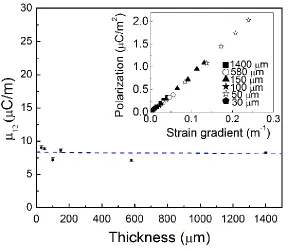
Figure 2.3 The transverse flexoelectric coefficient µ12 and the measured relationship between flexoelectric polarization and strain gradient (insets) in the BST microcantilever with different thicknesses. ... 27 Figure 2.4 Effective piezoelectric coefficients f

33 ef

d of piezoelectric bimorphs and flexoelectric microcantilevers as a function of thickness h under a constant length-to-thickness ratio (l/h = 50). ... 29 Figure 2.5 (a) Diagram of sample assembly for converse flexoelectric measurement of the shear strain along x1 direction generated by the electric filed gradient along x3 direction. (b) Schematic deformation of the trapezoid sample in the lateral mode. ... 33 Figure 2.6 Schematic view of a trapezoid sample with the voltage applied from side to side, (a) electric field line and equipotential distribution. O is the intersection point between the two extension lines of the slope side of the sample; (b) electric field gradient distribution; (c) electric field direction variation in arbitrary pitch arc r position. ... 36 Figure 2.7 Finite element simulation with COMSOL; areas with different color represent the magnitude of the calculated electric field gradient distribution within the trapezoid... 38 Figure 2.8 (a) Driving voltage, (b) measured displacement and (c) filtered displacement as a function of time for sample I. ... 41 Figure 2.9 Face displacement measured using a laser vibrometer as a function of voltage in room temperature for BST samples: (a) rectangle; (b) trapezoid 62°; and (c) trapezoid 46°. The green points are the second harmonic displacement associated with the electrostrictive effect. The blue points stand for the displacement associated with the piezoelectric and flexoelectric effect. The solid line is a guide to the eye. (d) Pure converse flexoelectric coefficient f1212 contribution extracted from the displacement subtraction in BST-II and BST-III as a function of voltage, respectively. The solid lines are the fitting slope of face displacement vs. voltage induced by net converse flexoelectric effect. ... 43 Figure 3.1 Circular hole in a plate subjected to uniaxial tension. ... 48 Figure 3.2 Strain and strain gradient distribution near the central hole in a aluminum plate (radius = 2.5 mm) with 1 MPa nominal tension stress. Distribution of (a) normalized εx, (b)

normalized εy, (c) ∂εx/ ∂y and (d) ∂εy/ ∂y. ... 50

Figure 3.4 Real time charge outputs from a BST micro-bar. ... 54

Figure 3.5 Relationships between the theoretically estimated and measured charge outputs with average strain gradients of the BST micro-bar SGS. ... 55

Figure 3.6 Loading diagram of four point bending (ASTM Standard)... 60

Figure 3.7 Curvature sensor configuration. ... 61

Figure 3.8 Beam curvature sensing: BST curvature sensor attached to beam. ... 63

Figure 3.9 Average strain distribution (color bar) on (a) top and (b) bottom surface of the curvature sensor. ... 64

Figure 3.10 Relationship between curvature transfer coefficient and the ratio of the epoxy bonding layer thickness and BST sensor thickness. ... 66

Figure 3.11 (a) Experimental set-up and (b) a close-up of the actual curvature sensor attached on beam. ... 67

Figure 3.12 Real time charge output from BST sensor 1. ... 69

Figure 3.13 Relationship between charge output and beam curvature-experimental results. 69 Figure 3.14 Moment-curvature relationship. ... 71

Figure 3.15 A mixed-mode crack inclined to a remote tensile field where a strain-gradient sensor is located at (r,θ) to measure strain gradient in the direction. ... 76

Figure 3.16 Definition of dimension parameters with SGS placement near the crack tip. ... 83

Figure 3.17 Normalized shift of averaged flexoelectric output as a function of normalized SGS position rc/L. ... 84

Figure 3.18 Photography of crack with two SGSs attached at different locations. ... 86

Figure 3.19 Comparison of empirical estimation of Mode-I stress intensity factor KI and measured results from two SGSs and one strain gauge. ... 88

Figure 3.20 Comparison of crack localization results from two SGSs and one strain gauge. 89 Figure 4.1 XRD spectrum of the wet etched BST (by BOE only). ... 100

Chapter 1

INTRODUCTION

1.1

1.1.1 Flexoelectric Effect

The flexoelectric effect describes the generation of an electric polarization response under a mechanical strain gradient (direct flexoelectric effect) [1] or the mechanical response under an electric field gradient (converse flexoelectric effect). In 1964, Kogan firstly discussed the electric polarization induced in a symmetric crystal by inhomogeneous deformation and introduced the concept of flexoelectricity.[2] The effect is schematically illustrated in Figure 1. As shown in Figure 1.1a, when the unit cell is under uniform strain, the centers of the negative and positive charges coincide with each other , and thereby resulting in a macroscopic zero net polarization. Consider the application of inhomogeneous strain depicted in Figure 1.1b, the displacement of the centers of the negative charge and positive charge differs from each other, creating a dipole moment in the direction opposite to the strain gradient, and hence resulting in a polarization.

In solid dielectrics, the flexoelectric effect can be written as ij

ijkl l

k P

x 

 



 (1.1)

where Pl is the flexoelectric polarization, µijkl the flexoelectric coefficient, 𝜺ij the elastic strain,

flexoelectric coefficient (µijkl) is linearly proportional to the dielectric susceptibility, which is

given as

ijkl ij kl

e a

   (1.2)

where χij is the susceptibility of the dielectric, γkl a constant material parameter tensor, e the

charge of the electron, and a the atomic dimension of the unit cell of the dielectric. Based on the rigid ion model, Tagantsev predicted four contributors to the flexoelectric effect, including static bulk flexoelectricity, dynamic bulk flexoelectricity, surface flexoelectricity and surface piezoelectricity. Through the theoretical study of a simple elemental cubic model for centrosymmetric materials, Resta suggested that the flexoelectric tensor is a bulk response of the solid, without surface contribution in the thermodynamic limit.[4] However, surface effect in the more complex symmetry group still remains unclear.

In the following part of this chapter, we will first review flexoelectricity in different materials, including the origin interpretations, flexoelectric coefficient definitions, and the corresponded experimental characterization methods. Secondly, typical structures for gradient generation under different flexoelectric modes will be introduced.

1.2 Flexoelectric Materials

Table 1.1 Numbers of the non-zero independent components of flexoelectric coefficients for solid materials in different point and Curie groups.[5, 6]

Point and Curie groups Numbers of independent components of µijkl

1, 1 54

2, m, 2/m 28

222, mm2, mmm 15

3, 3 18

32, 3m, 3m 10

4, 4, 4/m 14

4mm, 42m, 422, 4/mmm 8

6, 6, 6/m, ∞, ∞/m 13

622, 6m2, 6/mmm, ∞2, ∞m, ∞/mm 7

23, m3 5

432, 43m, m3m 3

∞∞, ∞∞m 2

1.2.1 Flexoelectricity in Solid Materials

extensively characterized and reported to be in the order of nC/m at room temperature,[14] which is significantly lower than measured results of those ceramics. As no direct experimental comparison exists for ceramic and single crystal of the same material, those uncertainty about the sources of measured flexoelectric effect cannot yet be clarified.

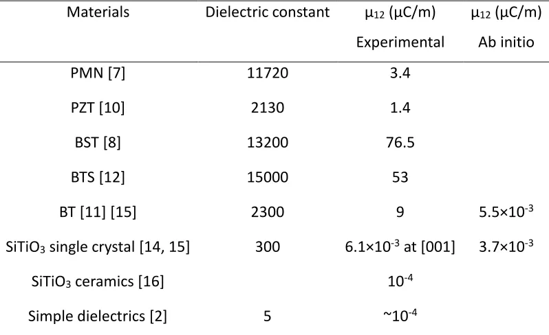
Table 1.2 µ12 of different materials at room temperature by experimental measurement and atomistic

estimation.

Materials Dielectric constant µ12 (µC/m)

Experimental

µ12 (µC/m)

Ab initio

PMN [7] 11720 3.4

PZT [10] 2130 1.4

BST [8] 13200 76.5

BTS [12] 15000 53

BT [11] [15] 2300 9 5.5×10-3

SiTiO3 single crystal [14, 15] 300 6.1×10-3 at [001] 3.7×10-3

SiTiO3 ceramics [16] 10-4

Simple dielectrics [2] 5 ~10-4

1.2.2 Flexoelectricity in Liquid Crystals

1 ( ) 3( )

Pen n e  n n (1.3)

with P representing the flexoelectric polarization, e1 and e3 denoting the splay and bend flexoelectric coefficients, respectively, and 𝒏 is the director of the curvature deformations. Values of the sum or the difference of the coefficients can be quantified by various indirect methods, i.e., analyzing optical effects produced by electric field induced director distortions. These methods require the understanding of other various independently measured material parameters, e.g., birefringence, anchoring energies, dielectric and elastic constants.[18, 19] Commonly measured coefficients for calamitic LC based on these methods are less than tens of pC m-1 and depends on the techniques used, which sometimes yield different values for even the same material.[20]Through a direct method via the electric current produced by periodic bending deformation of the LC’s bounding surface, Harden et al. recently reported a giant e3 of 35 ×10-9 _{C/m in the bent-core nematic LC,[21] which is three orders of magnitude greater} than those of traditional calamitic nematic LCs. This high value shows a good agreement with the measurements of the converse flexoelectric effect—an electric field induced mechanical

Figure 1.3 Schematic experimental setups for (a) direct [21] and (b) converse [23] flexoelectric effect measurement of LC.

1.2.3 Flexoelectricity in Polymers

the trapezoid shape film is due to a combination of piezoelectricity and flexoelectricity. By ruling out the piezoelectric contribution, μ11 of the PVDF was derived to be 81.5 μC/m.[26] However, the results undergo the criticism of poor linearity or negative slopes,[25] which contradicts the definition of flexoelectricity. In another work conducted by the same research group, effective transverse flexoelectric coefficient of PVDF films was investigated based on a bending test. Polymer film with a grounding electrode and top point electrode was bonded onto a cantilever beam to form a unimorph structure. Effective flexoelectric coefficient was calculated to be about 35 μC/m.[27] Different from the free standing cantilever method,[7] the piezoelectricity may be coupled in this unimorph structure because the asymmetric strain distribution in the film could not cancel out the piezoelectric effect. Chu et al. recently studied flexoelectricity in several thermoplastic and thermosetting polymers (including PVDF, oriented PET, polyethylene, and epoxy) by adopting the free standing cantilever bending test with a full covered top electrode.[28] The flexoelectric coefficients of these polymers are found to be of the order of 10-9 ~ 10-8 C/m, without an obvious dependence on dielectric constant of polymers.

1.2.4 Flexoelectricity in Biomembranes

exhibit flexoelectricity, whose direct effect denotes curvature-induced area membrane polarization and converse effect represents electric field-induced membrane curvature changes. For the curvature-induced membrane polarization the phenomenological expression by Petrov in 1975 reads[29]

1 2

1 1

( )

S

P f

R R

  (1.4)

where PS is the electric polarization per unit area (in C/m), R1 and R2 are the two principal radii

of membrane curvature[30] and f is the area flexoelectric coefficient[28], typically in the order of electron charge.

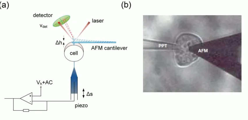
(BLM).[33] Voltage-induced membrane motions in cells can be investigated by using an atomic force microscope (AFM).[34, 35] The setup is shown in Figure 1.4. To characterize the opening of voltage-gated ion channels and membrane bending of the HEK293 cell, a holding potential Vh (-60 mV) and AC carrier voltage of ±10 mV at 66 Hz were applied to the cell by the patch clamp amplifier. AFM cantilever was pressed against the membrane to monitor the nanometer range normal movement of the membrane.

1.3 Flexoelectric Structures

In order to generate different strain gradient components and collect the corresponding electric outputs, specific mechanical structures and electrode configurations need to be adopted. In this section, three typical structures for axial, transverse and shear mode flexoelectric applications will be introduced, accompanied with a brief analysis.

1.3.1 Axial FE Structures

Truncated pyramid structures have been employed exclusively for μ11 characterization of various materials. As shown in the Figure 1.5(a), consider a truncated pyramid block with square cross-section, the upper face has a side of length a, and the lower a length b and linear sidewall has a depth of h. Under external loading F, strain distribution along the vertical axis of symmetry (x3 axis) is inhomogeneous. The flexoelectric polarization along z axis (P3(z)) can be derived as[1]

3

3( ) 2 11 11

( )

b a h

P z F

b a a z h s       (1.5)

where s11 is the mechanical compliance component. To compare with the performance of piezoelectric materials, effective piezoelectric coefficient of flexoelectric structures ( f

1.3.2 Shear FE Structures

If a shear stress is applied onto the truncated pyramid structure instead of a normal stress, shear flexoelectric component can be produced based on the relationship:

13 44 1

3

x

P  



 (1.7)

It should be noted that the polarization is along the x1 axis and hence electrodes need to be patterned accordingly for electric charge collection, as illustrated in Figure 1.5(b). Polarization and effective piezoelectricity of shear mode truncated pyramid has the similar expression as that of axial mode structure, except replacing the normal compliance and flexoelectric components into their shear counterparts.

1.3.3 Flexural FE Structures

Transverse strain gradient can be easily generated through beam bending. The axial strains in opposite surfaces have reverse orientations, resulting in a strain gradient along the thickness direction. Taking the cantilever as shown in Figure 1.5(c) for example, the effective piezoelectric coefficient can be estimated to be[36]

2 eff 12 11

3 33

6 h

s l

d   

 (1.8)

Figure 1.5 Basic structures of flexoelectric accelerometers (yellow layers represent the electrodes on the flexoelectric components).

1.3.4 Flexoelectric Composite Structures

resulting in the charge separation. The first demonstration of this possibility was reported by Zhu et al..[40] A 3×3 BST truncated pyramid array in millimeter scale was fabricated and the effective d33 constant was measured to be 6.0±1 pC/N. Specifically, the effective piezoelectric coefficient has a scaling effect for a certain flexoelectric geometry, i.e. truncated pyramid units. [1] Fu et al. reported the experimental studies of the gradient scaling phenomenon in two flexoelectric piezoelectric composites at the microscopic scale.[41] The flexoelectric phases were square truncated pyramid BST units with the height of 50 µm and 100 µm. Through converse piezoelectric response under 100 Hz, d33 values were measured to be 41±5 pC/N and 19±3 pC/N, respectively. The results suggest that by further decreasing the scale size, the flexoelectric mechanism may provide an alternative route to lead-free piezoelectricity with properties comparable to the widely used PZT ceramics.

Flexoelectricity associated piezoelectric composite could exhibit different properties compared with conventional piezoelectric materials. Due to the thermodynamically equivalence, piezoelectric materials usually have direct and converse effect simultaneously. The reciprocity could bring lots of unwanted harmonic signals in transducer applications.[42] Flexoelectric piezoelectric composite, on the contrary, could be used to separately control the direct and converse piezoelectric effects by specifically choosing the components materials, showing the potential advantage over piezoelectric materials.[43] Consider a two phase flexoelectric piezoelectric composite, if two phases possess the same dielectric property but different elastic properties, only electric field gradient can be generated in the flexoelectric components, thus this composite exhibits converse piezoelectricity but not the direct effect. In contrast, the composite in which two phases own the same elastic performance but different dielectric properties could only exhibit direct piezoelectricity. Chu et al. proposed a flexure mode composite (as shown in Figure 1.7) based on BST ceramics sheet with fine tungsten wires asymmetrically distributed on two sides.[44] Giant non-resonance f

33 ef

Figure 1.7 Cross section of a flexure mode composite using fine tungsten wires to induce strong transverse strain gradient.[44]

1.4 Limitations of Current Studies

On the other side, due to the scale effect of the flexoelectricity which is embedded in the gradient term, flexoelectricity would become more prominent at micro/nano size. Current publication only involves the flexoelectricity induced polarization alternation of piezoelectric thin film. Study of pure flexoelectric micro/nano structures without the interference of piezoelectricity is not yet reported. Due to the tangling of piezoelectricity and flexoelectricity in those studied thin films, the real flexoelectric contribution is difficult to be clarified. To directly demonstrate the enhanced flexoelectric effect at micro/nano scale, non-piezoelectric materials should be used. In addition, other various flexoelectric nano structures exist and can be exploited for sensing applications.

1.5 Dissertation Outline

With these considerations, the main goal of this research is to investigate the strain gradient sensing application of flexoelectric effect with ferroelectric materials, and to demonstrate the enhanced properties of micro/nano flexoelectric structures which lay down the foundation of future flexoelectric micro/nano devices. The dissertation consists of five chapters and references. Each chapter is briefly described as follows.

under an electric field gradient. Chapter 3 introduces the strain gradient sensing applications of flexoelectric sensors. The flexoelectric strain gradient sensors (SGS) were designed, prototyped and attached close to a circular hole on an aluminum plate. It was demonstrated that the flexoelectric SGS could accurately read out the strain gradient information in the plate under loading. This also enlightened a novel application of flexoelectric SGS for measuring the curvature of mechanical structures. The experiment was conducted by attaching the SGS to the side surface of a plate under four point bending. Furthermore, strain gradient can be a more sensitive measurand compared with strain in crack detection application. SGS was successfully utilized for monitoring the location of a premade crack. In the reverse way, SGS could offer a new avenue for characterizing the stress intensify factors of mechanical structures.

Chapter 2

FLELXOELECTRIC COEFFICIENTS MEASUREMENT

2.1 Introduction

To utilize the flexoelectric materials for sensing applications, it is essential to have flexoelectric coefficients of the materials corresponding to the functioning mode. Similar with piezoelectric coefficients measurement, the flexoelectric coefficients can be quantified through either direct or reverse means. In this chapter, direct transverse flexoelectric coefficient and converse shear flexoelectric coefficient measurement methods were investigated. The longitudinal flexoelectric coefficient can be measured in the similar way with the shear flexoelectric coefficient. The only diffidence exists in the electrode layout thus the electric field distribution. Based on these two methods, a comprehensive flexoelectric coefficients values for isotropic materials, e.g. BST ceramic, can be obtained, which can be the foundation for further applications.

2.2 Direct Measurement of µ12

2.2.1 Introduction

top and bottom surfaces. Even the material possesses piezoelectricity, the piezoelectric contribution from two sides of the neutral plane can be canceled out due to the reverse signs of the axial strain and the symmetric geometry. We adopted the similar method here to measure the BST ceramic beams with different thicknesses.

2.2.2 Sample Preparation

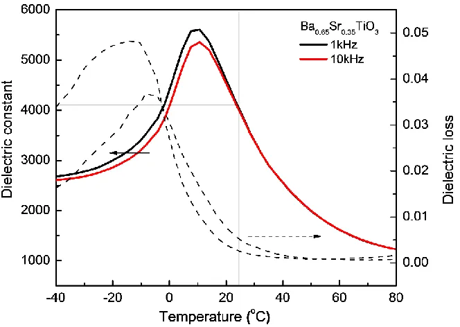
Figure 2.1 Dielectric constant and dielectric loss of prepared BST samples as function of temperature.

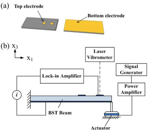
Figure 2.2 (a) Typical electrode configuration. (b) Experimental setup for the measurement of flexoelectric coefficients.

2.2.3 Measurement Method

The flexoelectricity measurements were carried out at room temperature with the experimental setup shown schematically in Figure 2.2(b). Strain gradient was generated in the samples along the thickness direction by a piezoelectric actuator, which was driven by a power amplifier (KH7602M) with a 2 Hz sinusoidal signal from a signal generator (AFG3000). The Polytec OFV-5000 laser vibrometer was used to measure the displacement at specific locations along the cantilever. The generated current was monitored using a lock-in amplifier (Stanford Research system, Mode SR830) with the reference signal from the signal generator. The generated polarization can then be calculated using the following equation:

3 2

I P

fA 

where I is the measured alternating current, A is the electrode area, f is the driving frequency of the actuator, and P3 is the polarization along the thickness direction.

By assuming the natural vibration of a cantilever beam, the nth mode shape can be written as [46]

1 1 1 1 1

cos cosh

( ) [(cos cosh ) (sin sinh )]

sin sinh

n n

n n n n n n

n n

l l

w x A x x x x

l l             

 (2.2)

where wn is the transverse deflection, l is the length of the beam, x1 is the axial distance from the clamped end to the measurement point. Here we only consider the fundamental mode (n=1), β1l= 1.875. A1 can be determined from the boundary condition, i.e., the measured vertical

displacement of the beam.

The transverse strain gradient along the thickness direction of the cantilever can be expressed as 2 11 1 2 3 1 ( ) w x x x    

  (2.3)

The resultant electric polarization from flexoelectric phenomenon can be written as 11 12 3 P x    

 (2.4)

With the measured I and w(x), transverse flexoelectric coefficient µ12 can then be calculated using Eq. 2.1 – 2.4.

the insert lines in Figure 2.3, was found to be about 8.5×10-6 C/m, which is much lower than the previously reported results (100 ×10-6 _{C/m) obtained from cantilevers with thickness of} sub-mm to millimeters [8],due to the low permittivity (4100) of the BST material at room temperature. Nevertheless, the confirmed scale independent flexoelectric coefficient holds great potential for flexoelectric N/MEMS.

Figure 2.3 The transverse flexoelectric coefficient µ12 and the measured relationship between flexoelectric polarization and strain gradient (insets) in the BST microcantilever with different thicknesses.

2.2.4 Scale Effect on Flexoelectric Structures

between physical parameters to the structural feature size and explains how physics work at different sizes. For example, electrostatic force is negligible in macro size compared with other kinds of forces like gravity. However, as the size diminish into micrometer level, the electrostatic force starts to be comparable to and even exceed the gravity. Such unique property has empowered the electrostatic effect to be applied to tremendous applications in micro electromechanical systems (MEMS), including inertial sensing, actuating, ultrasound transducer applications, etc.[48]

Flexoelectricity also exhibits such a favorable scaling effect as feature size shrinks down, which is inherited from the scaling nature of the mechanical strain gradient or electric field gradient. If the aspect ratios of the truncated pyramid and cantilever are set to be constant, the effective piezoelectric coefficients given in Eq. 1.6 and Eq. 1.8 will be reversely proportional to the structural thickness. To make a comparison between flexoelectric unit and piezoelectric counterpart, bending structure is used here as an example. The f

33 ef

d of a bimorph piezoelectric bender subjected to a perpendicular external tip force can be written as [49]

2 31

33 2

3 eff d l d

h  

 (2.5)

where d31 is the transverse piezoelectric coefficient of piezoelectric materials, l´´ the length of the bimorph and h´´ the thickness of the bimorph. The calculated f

33 ef

d of BST microcantilevers compared to those of ZnO thin film, PZT thin film (sol-gel, sputtering), potassium sodium niobate (KNN) thin film and lead magnate niobate-lead titanate (PMNT) single crystal cantilever bimorphs, are shown in Figure 2.4 as a function of thickness (The length to thickness ratio (l/h) was set to be a constant value of 50). Note that f

33 ef

calculation for BT,[50] though similar size dependent effective piezoelectric properties can be observed. Piezoelectric coefficients of conventional piezoelectric materials are given in Table 2.1. It can be observed that effective piezoelectric coefficient of flexoelectric cantilever became higher than those of well-known piezoelectric bimorphs when the thickness of cantilevers is scaled down to sub-micrometers, which can be further increased using optimized BST ceramics (e.g. µ12= 8.5×10-6 C/m [36] vs. the highest reported µ12= 100×10-6 C/m of BST [8]). Clearly, significantly enhanced effective piezoelectricity can be obtained with flexoelectric (FE) micro/nano-structures, considering the scale effect of flexoelectricity.

Figure 2.4 Effective piezoelectric coefficients f 33

ef

Table 2.1 Piezoelectric coefficients of conventional piezoelectric materials.[51, 52]

Piezoelectric materials d31 (pC/N)

ZnO thin film -5

PZT thin film (Sol-gel) -82

PZT thin film (Sputtering) -53

KNN thin film -20

PMNT single crystal -1000

2.3 Converse Measurement of µ44

High level of direct flexoelectric effect was found in high permittivity perovskites.[53] Intriguingly, the enhancement is 4 to 5 order larger than that of theoretical predictions. Moreover, PZT thin film[54] and soft polymer polyvinylidene fluoride (PVDF)[25] were also reported to have a large pure polarization when being bended.

but disappears in high symmetry crystals. For example, in a triclinic crystal, the number of non-zero independent components of fijkl is 54 while 36 for Mijkl. But for cubic or isotropic

crystals, both ijkl and Mijkl have the same non-zero components expressed as f1111, f1122, f1212

and M1111, M1122, M1212.

For most non-piezoelectric materials, Mijkl always plays a leading role for the contribution of

strain. In terms of mathematics, a non-zero ∂Ei/∂xj must be accompanied with E_i2, thus f1111 component coexists with M1111 effect. In Fu’s measurement,[55] the flexoelectric strain is more than two orders smaller than electrostrictive strain, rendering it difficult to separate f1111 from M1111. However, f1212 can exist alone when E₁/ x₃ 0, E E_{1 3} 0 or can be a dominant contributor to a shear strain when E₁/ x₃ 0, E E_{1 3} 0. In other words, a unidirectional electric field distribution is of high significance. Here, we underline the word distribution, which stands for the orientation variation in a board range of material. In this study, we experimentally verify the pure converse flexoelectric effect by applying a directional electric field E1, accompanied with a small E3 component, as well as a large gradient ∂E1/∂x3 so that the electrostrictive strain can be minimized in generating shear strain S13.

2.3.1 Measurement Method

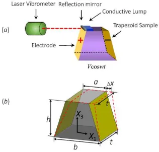
distributed along the height direction x3 due to the distance variation along direction x1. The measurement setup was laid down on a float optical table (Newport, ATS, Irvine, CA) to eliminate the vibrational noise. The AC voltage was generated by a power amplifier (Trek, 2220, Lockport, NY) under the excitation from a function generator (Tectronix, AFG3101, Lake Mary, FL). As suggested in [6], the symmetry of the cubic materials permits only shear strain S13, which is generated by ∂E1/∂x3 due to the coupling of f1212. To measure this shear strain, the bottom surface of the sample was clamped on the table and a reflective tape was attached to the top surface of the sample as a mirror for incident laser. The deformation along x1 direction was measured using a high resolution (<10 pm) laser vibrometer (Polytec, OFV-5000, Irvine, CA) and a lock-in amplifier (Stanford Research System, SR830, Sunnyvale, CA). Based on the measured shear deformation as illustrated in Figure 2.5b, the pure shear strain can be calculated as

5 2 13

x

S S

h



  (2.6)

Figure 2.5 (a) Diagram of sample assembly for converse flexoelectric measurement of the shear strain along x1 direction generated by the electric filed gradient along x3 direction. (b) Schematic deformation of the trapezoid sample in the lateral mode.

r

V E

r

 (2.7)

where r is the radius of the scallop and θ is the angle of the scallop. Thus, the electric field is not homogeneous in light of the space curvature of the electric field line. In this case, an electric filed gradient along the longitudinal direction (x3) is generated, as shown in Figure 2.6b. In addition, the angle between the electric field and x1 axis changes from -θ/2 to θ/2 across the whole region due to the geometric relationship as illustrated in Figure 2.6c. Hence, the average electric field component for an arc with the angle of θ at the radius of r in the transverse direction E₁ can be obtained as

/ 2 / 2 1

/ 2 / 2

sin / 2 cos

/ 2

r r

E d E d E

            





whereis the arbitrary vertex angle of the arc. In order to simply the calculation, the trapezoid sample was prepared with smooth side surfaces and rectangle top and bottom surfaces so that the average electric field E1 along the thickness gradient is

2

1 1

3 3

sin / 2

( )

( / 2)

b

a

E E V V

dx

x x h b a





 _  _{ }





where a and b are the side length of the top and bottom surface of the sample (Figure 2.5b), respectively.

Eq. 2.9 can be further simplified as Eq. 2.10 when  is equal or lower than  (the coefficient equals to 0.95)

1 3

1

( )

E V V

x h b a

 _{ }

Figure 2.6 Schematic view of a trapezoid sample with the voltage applied from side to side, (a) electric field line and equipotential distribution. O is the intersection point between the two extension lines of the slope side of the sample; (b) electric field gradient distribution; (c) electric field direction variation in arbitrary pitch arc r position.

Moreover, the electric field component E3 will, in principle, exist along with E1 according to the above analysis. Nevertheless, the productof E1•E3 is zero as interpreted in Eq. 2.11, so that it may not yield a shear strain coupled by electrostrictive constant M1212.

/ 2 / 2

1 3

/ 2 / 2

cos sin 0

r r

E E d E E d

 

 

   

 

 





Figure 2.7 Finite element simulation with COMSOL; areas with different color represent the magnitude of the calculated electric field gradient distribution within the trapezoid.

Table 2.2 Dimension of BST samples. Sample Cross

Section Shape (x1-x3 plane)

Vertex Angle (x1-x3 plane)

degree

Top Length

x1 a(mm)

Bottom Length

x1 b (mm)

Height x3

h (mm)

Thickness x2 t (mm)

BST I Rectangle 90 3.64 3.64 3.03 0.67

BST II Trapezoid 62 1.83 5.05 3.03 0.67

2.3.2 Results and Discussion

The measured face displacements of samples BST-I, BST-II and BST-III as a function of voltages ranged from 200 V to 700 V at 10 Hz are shown in Figure 2.9a ,b and c, respectively. A visible 20 Hz response was found in all of the samples, displaying with a quadratic regulation in plot. In principle in this experiment, irrespective of the symmetry of the sample, all the possible contributions to shear strain S13 can be expressed as

1

13 113 1 1212 1212 1 2 13 13 13

3

cos E cos cos cos ( ) ( ) ( )

S d E t f t M E E t t S P S F S M

x









     



(2.12)

domains,[59] which may be one possible reason for the existence of piezoelectric responses in BST samples.

On the other side, in Fu’s experiment,[55] the driven frequency of the power amplifier was 400 Hz. It is possible that the output waveform of the power amplifier was distorted and hence, was not a standard cosine function at such a high driven frequency. In this case, the first harmonic signal is unavoidably influenced by the coupling of electrostrictive effect. As interpreted by Fu et al., the small DC voltage shifts n generated by the power amplifier, resulting in a first harmonic response 2MijklnV₁cost. In our experiment, the driven frequency

Figure 2.8 (a) Driving voltage, (b) measured displacement and (c) filtered displacement as a function of time for sample I.

For rectangular sample BST-I, x V( ) is only derived from the piezoelectric displacement contribution P

113 113 1

2

( ) 2 ( ) d h

x V d E z dz V

W

 

_

As for the trapezoid sample II and III, x V( ) is expressed as

1 1

113 1 1212 113 1212

0 0

( )

( ) 2 ( ( ) ) 2 2

2( ) cot

h h

E z V E

x V d E z f dz d dz f dz

z a h z  z

          







2( ) cot 2

h

V b

d dz d V

a h z a



 

 



1

1212 1212 1₀ 1212 0

sin / 2 1 1

( )

/ 2

h

h

E

f dz f E f V

z a b

 

 _{  }





Figure 2.9 Face displacement measured using a laser vibrometer as a function of voltage in room temperature for BST samples: (a) rectangle; (b) trapezoid 62°; and (c) trapezoid 46°. The green points are the second harmonic displacement associated with the electrostrictive effect. The blue points stand for the displacement associated with the piezoelectric and flexoelectric effect. The solid line is a guide to the eye. (d) Pure converse flexoelectric coefficient f1212 contribution extracted from the displacement subtraction in BST-II and BST-III as a function of voltage, respectively. The solid lines are the fitting slope of face displacement vs. voltage induced by net converse flexoelectric effect.

sample. Linear fitting of the F induced displacement yields the converse flexoelectric coefficient f1212 to be 9.3×10-16 _m2_{/V and 1.18×10}-15 _m2_{/V for Sample II and Sample III,} respectively. The less common used unit m2/V can be converted to the nominal unit C/m by removing the factor of elastic constant. Generally, the elastic compliance constant s1212 of BST ceramics is around 8.5×10-12 m2/N,[60] by which the stress related flexoelectric constant 1212 is estimated to be 110 C/m (Sample II) and 138 C/m (Sample III). We note that the minus slope of the high linearity line stands for the deformation direction induced by electric field gradient, which is different from the piezoelectric deformation direction for this material. This converse flexoelectric coefficient is similar to the direct result 1111 (120 C/m) observed in the same materials.[40] It should be noted that the materials used here exhibit much higher dielectric permittivity compared with that used in the previous section, thus higher flexoelectric coefficients. As demonstrated in previous work, the relationship among the non-zero dependent components of the flexoelectric coefficients in isotropic crystals is expressed as 1212=1/2(1111-1122).[6] In this case, the value of the 1212 is half of the subtraction between

1111 and 1122 due to the high symmetry of the materials. In rigid ceramic materials, generally,

experiment firstly observed the shear flexoelectric data, being consistent with the theoretical prediction.

2.4 Summary

In this chapter, the scaling effect of flexoelectricity was studied using BST microcantilever beams with the thickness down to 30 μm. The measured transverse flexoelectric coefficient μ12 of ~8.5 μC/m remains constant for microcantilevers with various thicknesses. The calculated effective piezoelectric coefficient effective d33 and electrical energy density of FE cantilever beams using the measured μ12 increase greatly with the decreasing beam thickness, promising for flexoelectric microcantilever sensing applications.

Chapter 3

STRIN GRADIENT SENSING IN STRUCTURAL HEALTH

MONITORING APPLICATIONS

3.1 Strain Gradient Sensing

3.1.1 Introduction

sensitive detection of strain gradient – the most sensitive measurand near the localized damage location.

3.1.2 Strain Gradient Sensor Design

To demonstrate the capability of SGS for accurately monitoring the strain gradient information in mechanical structures, we attached it onto a round-hole structure which has a simple and precise analytical expression of the stress distribution near the perimeter, resulting in known strain gradient values as the reference.

at the electrodes with the configuration shown in Figure 3.1. Coaxial wires were bonded to the sidewall electrodes using silver paste to eliminate the external noise. The positive wire connected the inner side relative to the central hole, while the ground wire to the outer side. Epoxy adhesive (Hysol EA 9359.3) was used to bond the BST micro-bar to the aluminum substrate. A pressure of 0.2 MPa was applied to ensure the flatness of the epoxy layer, which was measured to be about 50 μm. The epoxy layer is also essential for insulating the sidewall electrodes from the metal substrate. The shear strength of the epoxy at room temperature is 1.03 GPa. The dimension of the aluminum substrate is 200 mm × 38 mm × 3.2 mm.

Figure 3.1 Circular hole in a plate subjected to uniaxial tension.

3.1.3 Strain Gradient Analysis

2 4 2

2 4 2

2 4

2 4

1 3 4

1 1 cos 2

2

1 3

1 1 cos 2 ,

2

r o

o

a a a

r r r

a a r r              _  _{ }   _{ }             _  _{ }  _{ }       (3.1)

where a is the hole radius, σo is the nominal stress induced by the uniaxial load at the location far away from the hole, r and θ are the coordinates of polar coordinate system, and σr and σθ

are the stress in radial and tangential directions, respectively. The stress distribution in Cartesian coordinates can be obtained through coordinate transformation and the corresponding strain components can be derived as

1

( )

1

( ) ,

x x y

y y x

E E           (3.2)

where v is the Poisson ratio, E is the Young’s modulus, εx, σx and εy ,σy are the strain and stress

Figure 3.2 Strain and strain gradient distribution near the central hole in a aluminum plate (radius = 2.5 mm) with 1 MPa nominal tension stress. Distribution of (a) normalized εx, (b)

normalized εy, (c) ∂εx/ ∂y and (d) ∂εy/ ∂y.

3.1.3.1 Shear lag effect

Since a finite thickness adhesive layer bonds between the BST micro-bar and the aluminum substrate, the strain or strain gradient in the substrate cannot be fully transmitted into the BST bar, known as the shear lag effect.[65] The derivation of the correction factor to account for shear lag effects was presented by Crawley and de Luis.[65] Consider a sensor with length lc,

bb, and thickness tb. Let the thickness of the bond layer be ts. Sensed relative strain (cb) has

the solution of [65]

1 cosh

sinh cosh 1 ,

sinh

c c

l

x x

l

       

 (3.3)

where G is the shear modulus of the bond layer material and  is defined as

2 4

.

c c c s b b b s

Gb G

Y t t Y b t t

   (3.4)

Substituting the dimensions to the equations, the correction factors of x and y can be

calculated individually and plotted in Figure 3.3. It can be observed that the maximum strain transmission happens at the center point of the sensor, while there is no strain transmitted to the sensor at the boundary. x at the center of the sensor was found to be on the order of 65%

Figure 3.3 Shear lag effects along sensor length and width.

With the transmitted strain gradient, the generated polarization in the BST micro-bar, induced by flexoelectric effect, can be written as

12 11

12 11

(

( ) )

, cy

cx y

y by x bx

P

y y

y y

 

 

   

 

 





 

 

 

 

(3.5)

where cx and cy are strain components in the BST micro-bar, bx and by are the strain

components in the aluminum substrates, and x and y are the correction factors in x and y

0 0 0 0 12 11 1 1 . c c

c cy c cy

cx cx

l _b l _b

c y

c c c

P dx dx

l b l b



















By multiplying the correction factor with strain gradient distribution in the aluminum, strain gradient distribution in the sensor can be obtained. The first part of the right hand side of (7), which arises from the average transverse strain gradient cx y, , is about 0.0036 m

-1 _{under the} nominal stress of 1 MPa, and the average transverse strain gradient cx y, without considering

the shear lag effect is about 0.0055 m-1. However, the second part of it, which is associated with the average longitudinal strain gradient _{cy y,} , is zero due to boundary condition of the shear lag effect. Hence the charge output (Q) can be given by

,

12 .

y cx y

c c c c

Ql t P l t

 

3.1.4 Experimental Results and Discussions

Figure 3.4 Real time charge outputs from a BST micro-bar.

Figure 3.5 Relationships between the theoretically estimated and measured charge outputs with average strain gradients of the BST micro-bar SGS.

theoretical evaluation if assuming a bonding thickness of 30 m. Secondly, deflection of the BST micro-bar from the tangency of the hole circumference will lead to inconsistence between the theoretical calculations and the real measurand. Besides, the non-ideal circular degree of the central hole may induce a disagreement between the theoretical strain model with the real strain distribution. Hence in order to eliminate the discrepancy between experimental output of BST micro-bar with theoretical analysis, future work will involve more precise control of the bonding layer thickness and uniformity, as well as better alignment of the BST micro-bar with the hole or other damage locations.

3.2 Curvature Sensing

3.2.1 Introduction

The term “curvature” of loaded structures is always of interest in the field of strength of materials and structures. However, in practice this physical parameter is difficult to be measured directly. It is known that the structural curvature and material strain are functionally related and one can usually be inferred from the knowledge of the other. Therefore, material strain has traditionally been measured to indicate the amount of structure deformation or loading [70] and there are numerous commercially available strain sensing devices that can be used to measure strain. However, strain measurement is not necessarily the best measurand in monitoring curvature. For example, plate-like thin elements are frequently used in modern infrastructure and aerospace structures. Strain is proportional to the thickness of the structure, and the strain magnitude decreases with the decrease in structural thickness under fixed curvature, leading to difficult strain measurements. In contrast, curvatures are constant throughout any structural section because the structural thickness is several orders of magnitude smaller than the radii of the curvature. Therefore, curvature measurements can be performed anywhere in a cross section, including the neutral plane even where there is no strain under pure bending.[71] Thus, there is a need of direct measurement of curvature, instead of indirect strain measurement, for health monitoring of thin slender structures.[72]

is very desirable. However, existing sensing technologies (e.g. strain gages, accelerometers, linear voltage displacement transducers) accompanied by interpretation algorithms are not effective for in-situ monitoring early damage because of its limited sensitivity, bandwidth, and accessibility to the hidden localized areas, let alone damage initiation and progression.[63] Apart from the above sensing techniques, if a sensor located on any location across the cross section can measure curvature directly, the sensor will provide an indication of any change in the stiffness of a structure subject to bending. Consequently, curvature sensors may be attractive for applications in structural integrity monitoring, such as bridges, or structural components of aircraft.

the light interferometric technique can also be used to measure bending curvature [82, 83], yet these systems are complex and expensive.

Taking account of the above considerations, flexoelectric sensor could provide a good avenue for the curvature sensing. In our study, a novel flexoelectric BST ceramic curvature sensor is proposed, for the first time, to measure bending curvature directly. It is studied theoretically and is tested experimentally by attaching the sensors to the side surface of an aluminum beam under four point bending condition to sense the beam curvature when the load monotonically increases. The main features of the flexoelectric curvature sensor reported include: direct curvature measurement, low frequency range applicability, high sensitivity, and no external excitation source needed. The flexoelectric curvature sensor is an alternative to strain measurement and is capable of on-line and in-situ structural integrity monitoring.

3.2.2 Curvature Sensor Design

3.2.2.1 Beam curvature

Figure 3.6 Loading diagram of four point bending (ASTM Standard).

In the pure bending mid-section which is the load span shown in the figure, the bending moment and axial strain can be given as

2 4

P l

M   (3.8)

3

3 2

x

M Pl

z z

EI Ebh

   (3.9)

where M is the bending moment and εx is the normal strain along x direction. From simple beam bending theory, curvature (k =1/R) is related to the bending moment (M) via the bending stiffness (EI), as given by the Euler bending formula:

3

d 3

d 2

x

M Pl

EI z Ebh



    (3.10)

3.2.2.2 Fabrication of curvature sensor

Similar SGS in the previous section is used here as the curvature sensor. Material properties and dimensions of BST sensor are listed in Table 3.1. Figure 3.7 shows schematically the curvature sensor with electrodes on the top and bottom surfaces (5 mm×0.4 mm). he is the thickness of epoxy bonding layer.

Table 3.1 Material and geometric properties of BST.

Symbol Description Value Units



E Young’s

modulus

153 GPa

 Poisson’s ratio 0.33 -

ls length 5 mm

bs width 1 mm

hs thickness 0.4 mm

3.2.2.3 Beam curvature sensing

The small size and light weight BST sensors can be attached to any location of a beam and exerts little impact on the host structure. In order to capture the beam curvature, two BST curvature sensors are attached onto the center side surfaces of an aluminum beam, located symmetrically with respect to its neutral axis, as illustrated in Figure 3.8. The sensor captures the beam curvature through strain gradient transferred through bonding epoxy. Coaxial wires were bonded to the top and bottom electrodes using silver paste to eliminate external noise. The positive wire was connected to the top electrode, while the ground wire to the bottom. The beam material properties and geometry are shown in Table 3.2.

Figure 3.8 Beam curvature sensing: BST curvature sensor attached to beam.

Table 3.2 Material and geometric properties of aluminum.

c Description Value Units



E Young’s

modulus

73 GPa

 Poisson’s ratio 0.33 -

l length 0.1 m

b width 0.05 m

h thickness 0.0127 m

and bottom surfaces are calculated as -2.90με and 2.88με, respectively. Then the average sensor strain gradient can be approximated by

bottom top s s x x x av z b       _  _ 

  (3.11)

where bs is the thickness of the BST sensor. Therefore the curvature transfer coefficient



s x av z       _   

 (3.12)

(a) (b)

Figure 3.9 Average strain distribution (color bar) on (a) top and (b) bottom surface of the curvature sensor.

By substituting Eq. 3.11 into Eq. 3.12, the curvature transfer coefficient is calculated as 0.582, which means only 58.2% of the actual beam curvature is transferred from aluminum beam to the curvature sensor through the bonding layer.

With the transferred strain gradient, the generated average polarization P₃ in the curvature