Genetic Mapping of Developmental Instability: Design, Model and Algorithm

DOI: 10.1534/genetics.107.072843

Genetic Mapping of Developmental Instability: Design,

Model and Algorithm

Jiasheng Wu,*

,†,‡

_{Bo Zhang,}

§

_{Yuehua Cui,}

‡

_{Wei Zhao,}

‡

_{Li’an Xu,}

§

_{Minren Huang,}

§

Yanru Zeng,

†

_{Jun Zhu* and Rongling Wu}

†,‡,§,1

*College of Agriculture and Biotechnology, Zhejiang University, Hangzhou, Zhejiang 310029, People’s Republic of China,†School of Forestry and Biotechnology, Zhejiang Forestry University, Lin’an, Zhejiang 311300, People’s Republic of China,‡Department

of Statistics, University of Florida, Gainesville, Florida 32611 and§The Key Laboratory of Forest Genetics and Gene Engineering, Nanjing Forestry University, Nanjing, Jiangsu 210037, People’s Republic of China

Manuscript received March 2, 2007 Accepted for publication March 27, 2007

ABSTRACT

Developmental instability or noise, defined as the phenotypic imprecision of an organism in the face of internal or external stochastic disturbances, has been thought to play an important role in shaping evo-lutionary processes and patterns. The genetic studies of developmental instability have been based on fluctuating asymmetry (FA) that measures random differences between the left and the right sides of bilateral traits. In this article, we frame an experimental design characterized by a spatial autocorrelation structure for determining the genetic control of developmental instability for those traits that cannot be bilaterally measured. This design allows the residual environmental variance of a quantitative trait to be dissolved into two components due to permanent and random environmental factors. The degree of de-velopmental instability is quantified by the relative proportion of the random residual variance to the total residual variance. We formulate a mixture model to estimate and test the genetic effects of quantitative trait loci (QTL) on the developmental instability of the trait. The genetic parameters including the QTL position, the QTL effects, and spatial autocorrelations are estimated by implementing the EM algorithm within the mixture model framework. Simulation studies were performed to investigate the statistical behavior of the model. A live example for poplar trees was used to map the QTL that control root length growth and its developmental instability from cuttings in water culture.

E

VERY live organism in the course of evolution is intricately equipped with developmental stability or canalization (Waddington1940) through collective mechanisms that buffer against the stochastic pertur-bations arising spontaneously from the cellular processes involved in the development of morphological struc-tures (Polak 2003). However, when stochastic pertur-bations of either environmental or genetic origin are beyond the capacity of the organism to produce a con-sistent phenotype, the organism will be forced to display some degree of developmental instability, manifested as the imprecision of developmental pathways and final morphological phenotypes (Waddington 1957; Zakharov1992; Palmer1994). Indeed, developmental instability embodies variation around the expected (tar-get) phenotype that should be produced by a specific genotype in a given environment, and the occurrence of developmental instability is due to small random er-rors accruing in development even when genetic and en-vironmental conditions are kept constant (Klingenberg 2004).

In general, developmental instability produces a subtle difference in each step of development. But increasingly more evidence has been observed that the accumulation of these minor differences may have played an important role in the ultimate formation and evolution of a complex trait (reviewed in Leamy and Klingenberg2005). In nature, developmental instabil-ity may negatively affect the fitness of a biological organ-ism (Badyaevet al. 2000) and the yield of an economic trait and its components, such as seed size, seed number and photosynthetic rate (Souzaet al. 2005), through the investment of extra energy to buffer against various environmental fluctuations that are internal and ex-ternal to an organism. A widely accepted view is that developmental instability will be higher in the more stressed populations compared to the control or un-stressed populations (Pankakoskiet al. 1992; Graham et al. 2000; Pertoldiet al. 2006). Given the fundamental importance of developmental instability, it is essential for understanding its genetic causes and consequences (Polak2003; Leamyand Klingenberg2005) and fur-ther exploring how it responds to natural or artificial selection within an evolutionary and ecological context (Clarke1998).

1_{Corresponding author:Department of Statistics, 409 McCarty Hall C,}

University of Florida, Gainesville, FL 32611. E-mail: [email protected]

Developmental instability is quantified by the amount of variation among phenotypes that would be produced by the same developmental blueprint under identical genetic and environmental conditions (Klingenberg 2004). In organisms like animals that display a bilateral symmetry, developmental instability is measured as fluc-tuating asymmetry (FA) that is due to random dif-ferences between left and right sides. Although FA is considered to be purely environmental in origin, it may also be under genetic control (Leamy1997; Markow and Clarke 1997; Palmer 2000; Fuller and Houle 2003). Empirical studies suggest that the heritability of FA is low (Pelabonet al. 2004), but in many cases it is significant, as observed in Scheineret al. (1991) and dem-onstrated by a meta-analysis of Møllerand Thornhill (1997a,b), although there is a controversy on this issue (Whitlock and Fowler 1997). Recent quantitative trait locus (QTL) mapping approaches (Lander and Botstein 1989; Lynch and Walsh 1998) have been performed to identify specific loci responsible for the variation of FA in mice (Leamyet al. 1998, 2002). These mapping studies allowed Leamy and Klingenberg (2005) to conjecture the nonadditive genetic architec-ture of FA composed of intralocus (dominance) and interlocus interactions (epistasis).

Plants, as organisms with modular construction, are very suitable subjects for detecting developmental in-stability caused by environmental disturbance. The anal-ysis of the asymmetry of plant structural traits can be used to determine deviations from the basic structural pattern, which is a measure of plant developmental in-stability. However, for important traits such as stemwood growth in forest trees and grain yield in crops, it is not possible to measure such asymmetry. Different from conventional FA measures, developmental instability for these traits can be measured by growing individual plants of the same genotype in a microsite with clonal rep-licates or recombinant inbred lines. Variation among phenotypes of different individuals within a clonal geno-type under a similar condition is thought to stem from developmental instability or noise.

In this article, we propose an experimental design based on genotypic replicates in space to map and es-timate the genetic effects of QTL on the developmental instability of a quantitative trait. A mixture model is constructed to separate different QTL genotypes in terms of observed marker information (Landerand Botstein 1989). The autoregressive model interpreted on a spatial scale is used to model the structure of the residual vari-ance matrix (Cressie1991). It assumes that the residual correlation between any two different copies of the same progeny genotype decays exponentially with the physical distance between these two replicates in the field. Also, the residual variance is postulated to be composed of two components due to permanent and random envi-ronmental factors. The random residual variance due to stochastic independent errors reflects the degree of

de-velopmental instability. The genetic control of devel-opmental instability can be determined by testing the difference in the random residual variance among QTL genotypes inferred from a molecular linkage map. The statistical model is constructed within the context of maximum likelihood and implemented with the EM al-gorithm (Dempsteret al. 1977). Simulation studies have been performed to investigate the statistical behavior of the model. We used a real example in poplars to validate the usefulness of the model.

THE MODEL

Experimental design: Consider a simple backcross

design in whichnprogeny are segregating in a 1:1 ratio at each locus. A genetic linkage map, aimed to identify segregating quantitative trait loci (QTL), is constructed with polymorphic markers genotyped through the ge-nome. Each backcross progeny is replicated with clones, recombinant inbred lines, or isogenic lines and planted in a randomized complete design. There are multiple replicates for each progeny planted in a plot. The number of replicates (R) can be small or large, depend-ing on the availability of materials. The shape of a plot can be a triangle, a rectangle, a square, and so on. With-out loss of generality, let each progeny have four copies laid out in a square plot with a loop 1/2/3/4/1 at a spacing ofd3dm. Thus, the physical distances between any two plants can be expressed as

d12¼d;for plants 1 and 2;

d23¼d;for plants 2 and 3; d34¼d;for plants 3 and 4;

d41¼d;for plants 4 and 1;

d13¼dpffiffiffi2;for plants 1 and 3;

d24¼dpffiffiffi2;for plants 2 and 4: ð1Þ

For other layouts, between-plant distances can always be calculated as long as the geometric shape of the plot and the number of copies are known.

Linear model:The phenotypic value of a quantitative

trait, yij, for progeny i at its jth replicate in a plot is

described by a linear model

yij¼ci1eij; ð2Þ

whereciis the genotypic value of progenyiandejis the

residual (or environmental) effect,eijN(0,s2).

Suppose there is a putative QTL in the backcross, with two genotypes,Qq (coded by 1) andqq (coded by 0), involved in the control of the trait. The genotypic value of progenyican be partitioned into two components, i.e., the genotypic value (mh) of QTL genotypeh(h¼1,

0) and the genetic effect (cijh) due to other loci rather

than the QTL under consideration. Because of the replicates of a progeny, the residual effect is partitioned into permanent (pi) and random environmental effect

yij¼

X1

h¼0

j_hm_h1cijh1pi1eij; ð3Þ

where jh is the indicator variable for QTL genotypes

defined as 1 for a considered QTL genotype and 0 other-wise,m_his assumed to be a fixed effect, andcijh,pi, and e_ijare assumed to be the random effects, withcijhN(0, s2

c),piN(0,s2p), andeijN(0,s2e).

Autocorrelation structure: Let yi ¼ {yij}Rj¼1 be the

vector of the observed value for the trait measured for progenyiplanted withRreplicates in a plot. Equations 2 and 3 are then written in matrix notation as

y_i ¼Fici1ei

¼X

1

h¼0

j_hFimh1Ficijh1Cipi1ei; ð4Þ

where Fi is an R-dimensional vector of all elements

equal to 1,Ciis anR-dimensional vector whose elements

describe the spatial positions of different replicates for progenyiwithin a plot,ei¼ feijg

R

j¼1, andei¼ feijg R j¼1.

TheR-dimensional residual covariance matrix of the phenotype vector (yi) among different replicates across

different progenies of the same QTL genotype is ex-pressed in terms of Equation 4 as

Si ¼FTiFis2c1Ris2p1Iis2e

¼FT

iFis2c1½ð1gÞRi1gIis2e; ð5Þ where matrixRispecifies the autocorrelation structure

of different replicates for progeny i within a plot, de-fined by the positions of replicatesCi(Cressie1991),

andIiis an identity matrix because the random

environ-mental effects are assumed to be independent among replicates.

Equation 5 partitions the variance within QTL geno-types into two parts, one being the genetic variance and the other being the residual environmental variance. The environmental variance is further partitioned into spatial and nonspatial components. The spatial com-ponent of the environmental variance is due to some permanent factors within a plot, such as moisture or nutritional gradients in a microsite. The nonspatial com-ponent of the residual environmental variance that does not depend on microenvironmental gradients is due to local unpredictable variability arising from random independent errors. The nonspatial component repre-sents the local variance of the residual error that is often called the ‘‘nugget variance’’ (Isaaks and Srivastava 1989). Thus, the relative magnitude of the spatial and nonspatial components, described by parameter g, re-flects the extent of the local variability due to devel-opmental instability. On the basis of this definition, we have the permanent environmental variances2

p¼(1

g)s2_{and the random environmental variances}2

e¼gs2.

The spatial covariance matrix can be structured by various statistical models, such as the first-order au-toregressive ½AR(1) model, in which the variance is assumed to be constant over different plant positions within a plot and the spatial correlation drops off ex-ponentially with the distance between plant positions, so that a distance ofdbetween plant positions leads to a correlation of rd

. Considering a square plot, we model the spatial correlation matrix for progenyiby

Ri¼

1 rd _rpffiffi2d _rd

rd _{1 r}d _rpffiffi2d

rpffiffi2d _rd _{1 r}d

rd _rpffiffi2d _rd ₁

2 6 6 6 4

3 7 7 7

5: ð6Þ

A similar modeling structure can also be used for other different layouts of the plot.

Likelihood function and computational algorithm: The likelihood function of the observed values (y) for the trait and marker information (M) can be expressed, by a mixture model (Landerand Botstein1989), as

LðVjy;MÞ ¼Y

n

i¼1

½-1jif1ðyiÞ1-0jif0ðyiÞ; ð7Þ

where V is the unknown vector including the QTL position, the QTL genotypic values (mh), the genetic

variance within QTL genotypes (s2

c), the permanent

environmental correlation (r), the residual variance (s2_{), and the proportion of the random residual} vari-ance to the total residual varivari-ance (g).

The mixture proportions, -1jiand-0ji, are the QTL

genotype frequencies in the backcross. Because each backcross progeny has known marker genotypes, the likelihood function will be expressed in terms of known groups of marker genotypes. Let the putative QTL be predicted by a pair of flanking markers that bracket the QTL. Thus, the QTL genotype frequencies should be expressed for each of the four possible marker geno-types. These so-called conditional probabilities of QTL genotype given marker genotypes are derived in terms of the recombination fractions between the QTL and two flanking markers. For a dense map, these condi-tional probabilities can be approximated by the ratio (u) between the QTL–marker over marker–marker recom-bination fractions. We thereby use u to denote the chromosomal location of the QTL within the marker interval.

The multivariate normal distribution probability of the trait for QTL genotype h (h ¼1, 0), fh(yi), is

ex-pressed as

fhðyiÞ ¼

1 ð2pÞR=2_jS

hj1=2

exp 1

2ðyiuhjiÞSh1ðyiuhjiÞT

;

where uhji¼Fimhis the vector of the genotypic values

hwithin a plot. We use Equation 5 to model the struc-ture of the covariance matrix in the above probability density function specifically for QTL genotypes. Assume that the QTL does not affect the spatial (permanent) residual variance, but it is responsible for the local (random) residual variance. Thus, by defining a QTL genotype-specific proportion of the local to total resi-dual variance,gh, and comparing its differences among

different QTL genotypes, we can test whether the de-velopmental instability of the trait studied is controlled by the hypothesized QTL.

The EM algorithm (Dempsteret al. 1977) is imple-mented to estimate the genotypic values and the pa-rameters that model the structure of the covariance matrix, all contained in vectorV¼(u,Q) withQ¼(mh, s2

c,gh,r,s2) (h¼1, 0). These unknown parameters can

be estimated by differentiating the log-likelihood func-tion of Equafunc-tion 7 with respect to each parameter, let-ting the derivatives be equal to zero, and solving the log-likelihood functions.

The log-likelihood function of the phenotypic values for a trait affected by a QTL is given by

logLðVjy;MÞ ¼X

n

i¼1

log½-₁jif1ðyiÞ1-0jif0ðyiÞ;

with the derivative with respect to any elementV‘in the

unknown vector

@ @V‘

logLðVjy;MÞ

¼X

n

i¼1

f1ðyiÞð@-1ji=@uÞ1f0ðyiÞð@-0ji=@uÞ -1jif1ðyiÞ1-0jif0ðyiÞ

1-1jið@=@QÞf1ðyiÞ1-0jið@=@QÞf0ðyiÞ -1jif1ðyiÞ1-0jif0ðyiÞ

¼X

n

i¼1

-1jif1ðyiÞð1=-1jiÞð@-1ji=@uÞ1-0jif0ðyiÞð1=-0jiÞð@-0ji=@uÞ -1jif1ðyiÞ1-0jif0ðyiÞ

1-1jif1ðyiÞð@=@QÞlogf1ðyiÞ1-0jif0ðyiÞð@=@QÞlogf1ðyiÞ -1jif1ðyiÞ1-0jif0ðyiÞ

¼X

n

i¼1

P1ji 1

-1ji @-1ji

@u 1

@

@Qlogf1ðyiÞ

1P0ji 1

-0ji @-0ji

@u 1

@

@Qlogf0ðyiÞ

;

where we define

P_hji ¼

-hjifhðyiÞ

-1jif1ðyiÞ1-0jif0ðyiÞ

; ð8Þ

which could be thought of as a posterior probability that progenyihas QTL genotypeh. We then implement the EM algorithm with the expanded parameter set {V,P}, whereP¼{Phji}. Conditional onP(the E step;

Equa-tion 8), we solve the log-likelihood equaEqua-tions

@ @V‘

logLðVjy; MÞ ¼0 ð9Þ

to get the estimates ofV(the M step). The E and M steps between Equations 8 and 9 are repeated until the

esti-mates converge to stable values that are regarded as the maximum-likelihood estimates (MLEs) of the parame-ters. A detailed procedure for the derivations of the MLEs is available upon request.

In practical computations, the QTL position param-eter can be viewed as a fixed paramparam-eter because a puta-tive QTL can be searched at every 1 or 2 cM on a map interval bracketed by two markers throughout the entire linkage map. The log-likelihood-ratio test statistic for a QTL at a particular map position is displayed graphi-cally to generate a likelihood map or profile. The geno-mic position that corresponds to a peak of the profile is the MLE of the QTL location.

HYPOTHESIS TESTS

The existence of QTL: On the basis of the MLEs of

two QTL genotypic values, we estimate the overall mean by ˆm¼ ðmˆ₁1mˆ₀Þ=2 and the additive genetic effect of the QTL on the trait byaˆ¼ ðmˆ₁mˆ₀Þ=2. This design allows us to test the existence of a QTL, regardless of whether it affects only the trait or its developmental instability or both. This can be tested by formulating the following hypotheses:

H0: a ¼0 andg1¼g0[g

H1: at least one of equalities above does not hold:

ð10Þ

The log-likelihood valuesL0andL1under H0and H1are

calculated. The test is performed with a log-likelihood-ratio statistic

LR¼ 2½lnL0ðm˜;g˜;r˜;s˜2jyÞ lnL1ðVˆjy;MÞ; ð11Þ where the tildes and hat stand for the MLEs under the null and the alternative hypothesis, respectively. The LR statistic is plotted against test locations and a high LR corresponds to the position of QTL. Because the QTL position under H0of hypothesis (10) is not identifiable,

the distribution of the LR calculated is unclear. An empirical approach for determining the critical thresh-old that does not depend on the distribution is based on permutation tests, as advocated by Churchilland Doerge (1994). By repeatedly shuffling the relation-ships between marker genotypes and phenotypes, a series of the maximum-log-likelihood ratios are calcu-lated, from the distribution of which the critical thresh-old is determined.

The effect of the QTL on the trait can be tested using the hypotheses as follows:

H0: a¼0

H1: a6¼0: ð12Þ

the QTL position under the null hypothesis is identifi-able, a case different from hypothesis (10). The genetic variance of the trait contributed by the detected QTL is the variance between the two QTL genotypes, calculated by

s2 g¼

1 4a

2_:

The total environmental variance is the summation of the residual environmental variance within each QTL genotype weighted by the frequencies of QTL geno-types, calculated as

s2_e¼ 1

2R2 FS1F T_1FS

0FT

:

Thus, the heritability of the trait explained by the QTL is calculated as

h2¼ s

2 g

s2_g1s2_c1s2_e:

Genetic control of developmental instability: After

the existence of a QTL for the trait is confirmed, it is essential to test whether this detected QTL triggers an effect on the developmental instability of the trait. We can first test whether the nonspatial local variation is significant by formulating the hypotheses

H0: g1¼g0 ¼0

H1: at least one of equalities above does not hold:

ð13Þ

If H0of hypothesis (13) is accepted, this means that all

the residual variance is contributed by the spatial vari-ance and that there is no varivari-ance due to developmental instability. By contrast, if the null hypothesis of the test

H0: g1¼g0 ¼1

H1: at least one of equalities above does not hold

ð14Þ

is accepted, this indicates that the nonspatial compo-nent,i.e., the nugget effect, is only a source for the re-sidual variance.

The genetic control of developmental instability is tested by

H0: g1 ¼g0

H1: g1 6¼g0: ð15Þ If H0 of hypothesis (15) is rejected, this suggests that

developmental instability is under significant genetic control. The LR values for hypotheses (13)–(15) can be thought to follow ax2_{-distribution with 2 or 1 d.f.,} re-spectively. For each QTL genotype, the proportion of the nonspatial variance due to developmental noise relative to the total residual variance is calculated by

Hh¼

ghðFIFTÞs2

FShFT

: ð16Þ

Thus, by comparingHhbetween the two genotypes, we

determine how the QTL detected for the trait affects its developmental instability.

APPLICATION

Material: We used a real example for QTL mapping

in poplar trees to demonstrate the usefulness of our model. The study material, as described in Wu et al. (2002), was derived from the triple hybridization of Populus (poplar),Populus deltoides, andP. euramericana, which is an interspecific hybrid betweenP. deltoidesand P. nigra. Of .400 triple hybrids, 90 were randomly chosen to establish a mapping population for marker analysis and QTL identification. Given the heterozygous characteristic of forest trees, analysis of this mapping population is based on a pseudotest backcross design (Grattapagliaand Sederoff1994), in which markers and QTL are heterozygous in one parent but not in the second parent. According to this design, two genetic link-age maps each based on the gene segregation of a dif-ferent parent were constructed with difdif-ferent types of molecular markers (Yinet al. 2002). Our analysis here is based on aP. deltoides(D)-specific linkage map.

Ramets from each of the progeny used to construct linkage maps were made to study their rooting capacity. The ramets were water cultured in a randomized com-plete block design with three different blocks and a four-tree square plot. Root numbers were counted and the length of each root was measured at five weekly intervals starting at day 7. The total root length of each cutting was then estimated. In this study, the total root lengths at the last measurement point were used. A total of 75 trees containing complete marker and trait data are used.

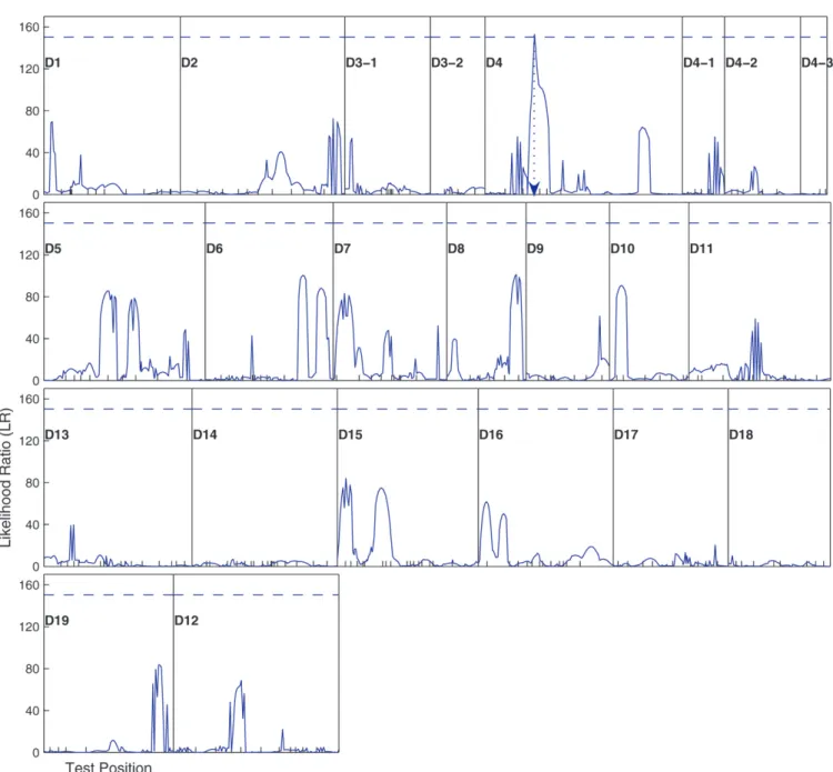
Results: The mapping model with an algorithm

The two subsequent hypotheses (12 and 15) were made to test whether this QTL triggers an effect on root length growth and the developmental instability of the trait, respectively. The testing results suggest that the QTL has a significant additive effect on the root length (Table 1), explaining 19.9% of the total phenotypic variance for the trait. In addition, this QTL also displays a significant effect on the developmental instability of root length, with the nugget parameters being different between the two QTL genotypes (0.802 and 0.094; Table 1). Developmental instability explains different propor-tions of the residual variance for two different QTL

ge-notypes, respectively, as calculated by Equation 16, with such a proportion being larger for the larger genotype (29.2%) than for the smaller genotype (5.9%).

Monte Carlo simulation: We performed simulation

studies to investigate the statistical properties of the model for mapping developmental instability QTL. We mimicked the poplar example by simulating the back-cross of a low sample size (n¼75). A linkage group of length 200 cM is constructed with 10 evenly distanced markers for this backcross. To investigate the influence of sample size on parameter estimation, we performed further simulation studies by increasing sample size to Figure1.—The profiles of the log-likelihood ratios between the full and reduced (no QTL) model for root length growth across

200 and 500. Each progeny from this backcross is planted with a square plot of four copies. Assume that a QTL located at 48 cM from the first marker at the left of the linkage group affects a normally distributed trait. With the given additive genetic effect of the QTL, along with the parameters that specify the spatial and non-spatial structure of the covariance matrix (Equation 5; Table 2), the phenotypic values of the backcross are simulated under different heritability levels (h2 _¼0.1 and 0.4). The spatial correlation is modeled by the AR model (Equation 6).

The simulated data are subjected to statistical analyses by the mapping model proposed. For a small sample size like the one used for the poplar example, the model provides reasonable but not excellent estimates for all the parameters (including the QTL position, QTL ef-fects on the simulated trait and its developmental insta-bility, and covariance-structuring parameters) when the heritability of the simulated trait is low (Table 2).

How-ever, as the sample size increases, the precision of pa-rameter estimation increases remarkably. As expected, these estimates are more accurate and more precise with a high heritability. The model appears to have high power for the detection of significant effects on devel-opmental instability, even for a low sample size and a low heritability level (Table 2).

DISCUSSION

Because developmental systems are inherently ‘‘noisy’’ and frequently subject to random fluctuations, consid-erable variation can be observed in the rates of develop-ment and morphology even among genetically identical individuals under the most uniform experimental con-ditions (McAdams and Arkin 1997). This so-called developmental noise or instability has been thought to be related to the fitness and evolution of the organism (Møllerand Swaddle1997). The study of the genetic

TABLE 2

The MLEs of the QTL position and effect and covariance-structuring parameters under the assumption of the genetic control of developmental instability derived from 100 simulation replicates

n h2

Position

(at 48 cM) m¼10 a¼1 g1¼0.4 g2¼0.8 r¼0.9 s2 _Power

0.1 75 49.48 10.013 0.928 0.337 0.767 0.870 4.634 81

(17.105) (0.170) (0.523) (0.224) (0.161) (0.129) (0.496)

0.1 200 48.16 10.005 0.951 0.361 0.789 0.879 4.612 100

(8.283) (0.120) (0.232) (0.150) (0.099) (0.089) (0.270)

0.1 500 47.52 10.004 0.992 0.387 0.794 0.894 4.631 100

(4.807) (0.062) (0.141) (0.107) (0.055) (0.063) (0.138)

0.4 75 47.08 10.010 1.002 0.326 0.773 0.869 0.754 100

(7.821) (0.073) (0.168) (0.209) (0.147) (0.121) (0.088)

0.4 200 48.38 9.997 0.989 0.374 0.803 0.894 0.763 100

(4.230) (0.048) (0.086) (0.150) (0.083) (0.093) (0.050)

0.4 500 47.78 10.001 1.001 0.386 0.795 0.896 0.771 100

(1.694) (0.029) (0.059) (0.106) (0.053) (0.068) (0.032)

The location of the QTL is described by the map distance (in centimorgans) from the first marker of the linkage group (100 cM long). The hypothesizeds2_{-value is 0.771 forh}2_{¼0.4 and 4.628 forh}2_{¼0.1. The square} roots of the mean squared errors of the MLEs are given in parentheses.

TABLE 1

The results of QTL mapping for rooting capacity and its developmental instability in a pseudotest backcross design of poplar

Marker interval AG/CGA-395d–CA/CCG-680d

ˆ

m sˆ2

c aˆ g1ˆ g0ˆ rˆ sˆ

2

MLE 1.683 0.101 0.552 0.802 0.094 0.934 0.568

LR 152.9

LRT 34.2

LRD 66.5

control of developmental instability has been the sub-ject of great interest in evolutionary and developmental biology (Klingenbergand Nijhout1999; Leamyand Klingenberg2005) and agricultural genetics (Wu1997). Traditional quantitative genetic approaches have been used to estimate the genetic variability and heritability of developmental instability measured as FA for bilateral traits. Specific QTL have been identified for FA in mice with molecular genetic linkage maps (Leamyet al. 2002). In this article, we have framed a general design to esti-mate QTL that affect developmental instability for those traits whose developmental instability cannot be mea-sured in terms of FA. We have derived a statistical model and a computational procedure for testing and estimat-ing the effect of QTL on developmental instability with the data collected from a field trial.

The idea behind our model is the incorporation of the spatial autocorrelation model into the QTL map-ping framework. We have implemented a common form of spatial autocorrelation (Cressie1991) that involves both spatial and nonspatial,i.e., local or ‘‘nugget,’’ com-ponents (Isaaks and Srivastava1989). Thus, rather than estimating all elements contained within the co-variance matrix, our model estimates a few key param-eters that model the structure of the covariance matrix. Spatial components result from some predictable mi-croenvironments within a plot, whereas nonspatial com-ponents result from local unpredictable perturbations. Thus, the proportion of nonspatial relative to spatial variances can be regarded as the degree of developmen-tal instability. We derived the EM algorithm to estimate the parameters that structure the covariance matrix. The derived algorithm is robust, as seen from results through simulation studies, in that the model provides reasonable estimates of genotypic effects and spatial pa-rameters over a range of space including different sam-ple sizes and heritability levels.

The new model has been employed to identify a QTL that affects rooting capacity and its developmental in-stability from cuttings of poplar trees in a controlled water culture laid in a square plot with three blocks. We have detected a significant QTL on a linkage group constructed by AFLP markers in an interspecific hybrid population of two poplar species (Yinet al. 2002). On the basis of previous quantitative and molecular genetic studies, rooting capacity is found to be under strong genetic control in woody plants (Wang et al. 1988; Wullschleger et al. 2005). Several QTL for fine or coarse root biomass traits have been mapped on specific chromosomal locations for hybrid poplars between P. trichocarpa3P. deltoides(Wullschlegeret al. 2005). A smaller number of the root QTL detected in this study may be due to a small sample size and/or possible C-effects, a common phenomenon in vegetative prop-agation (Stelzeret al. 1998), that describe variation in trait performance among different ramets from dif-ferent tree positions. A structuring model for

approxi-mating the dependence of ramets can be proposed to remove C-effects that may have confounded the esti-mates of the genetic parameters in the poplar example. As a first conceptual exploration of its kind, our map-ping model was formulated in terms of interval mapmap-ping and it should be powerful to detect unlinked QTL for a quantitative trait. Its capacity to separate multiple linked QTL can be improved through the combination of in-terval mapping and partial regression analysis on all the markers except for the two that flank the QTL. This so-called composite interval mapping (Zeng 1994) that has proven to increase the resolution of QTL mapping can be readily integrated with our mapping model to more precisely identify positions and effects of QTL that control the developmental instability of a quantitative trait. Another immediate issue is to incorporate the effects of QTL3environment interactions on developmental instability when the trial is conducted under multiple different sites. Such a multisite trial is needed to avoid the inflated estimate of the genetic control of develop-mental instability. Our developdevelop-mental model and its extensions will prove their value to draw a detailed pic-ture of the developmental instability of complex phe-notypes for a variety of organisms in plants and animals.

We thank two anonymous reviewers for their constructive comments on this manuscript. This work is partially supported by grants (09-95671 and 30671704) from the National Natural Science Foundation of China and from the National Science Foundation (0540745).

LITERATURE CITED

Badyaev, A. V., K. R. Foresmanand M. V. Fernandes, 2000 Stress

and developmental stability: vegetation removal causes increased fluctuating asymmetry in shrews. Ecology81:336–345. Churchill_{, G. A., and R. W. D}oerge_{, 1994 Empirical threshold}

values for quantitative trait mapping. Genetics138:963–971. Clarke_{, G. M., 1998 Developmental stability and fitness: the}

evi-dence is not quite so clear. Am. Nat.152:762–766.

Cressie, N. A. C., 1991 _{Statistics for Spatial Data}. John Wiley & Sons,

New York.

Dempster, A. P., N. M. Lairdand D. B. Rubin, 1977 Maximum

like-lihood from incomplete data via EM algorithm. J. R. Stat. Soc. Ser. B39:1–38.

Fuller_{, R. C., and D. H}oule_{, 2003 Inheritance of developmental}

instability, pp. 157–186 inDevelopmental Instability. Causes and Con-sequences, edited by M. Polak_{. Oxford University Press, New York.}

Graham, J. H., D. Fletcher, J. Tigueand M. McDonald, 2000 Growth

and developmental stability ofDrosophila melanogasterin low fre-quency magnetic fields. Bioelectromagnetics21:465–472. Grattapaglia, D., and R. R. Sederoff, 1994 Genetic linkage maps

ofEucalyptus grandis and Eucalyptus urophylla using a pseudo-testcross: mapping strategy and RAPD markers. Genetics 137:

1121–1137.

Isaaks, E. H., and R. M. Srivastava, 1989 Applied Geostatistics. Oxford

University Press, New York.

Klingenberg, C. P., 2004 Dominance, nonlinear developmental

map-ping and developmental stability, pp. 37–51 inThe Biology of Genetic Dominance, edited by R. A. Veitia. Landes Bioscience, Austin, TX.

Klingenberg, C. P., and H. F. Nijhout, 1999 Genetics of

fluctuat-ing asymmetry: a developmental model of developmental insta-bility. Evolution53:358–375.

Lander_{, E. S., and D. B}otstein_{, 1989 Mapping Mendelian factors}

underlying quantitative traits using RFLP linkage maps. Genetics

121:185–199.

Leamy, L., 1997 Is developmental stability heritable? J. Evol. Biol.

Leamy, L. J., and C. P. Klingenberg, 2005 The genetics and evolution

of fluctuating asymmetry. Annu. Rev. Ecol. Evol. Syst.36:1–21. Leamy, L. J., E. J. Routmanand J. M. Cheverud, 1998 Quantitative

trait loci for fluctuating asymmetry of discrete skeletal characters in mice. Heredity80:509–518.

Leamy_{, L. J., E. J. R}outman_{and J. M. C}heverud_{, 2002 An epistatic}

genetic basis for fluctuating asymmetry of mandible size in mice. Evolution56:642–653.

Lynch_{, M., and B. W}alsh_{, 1998 Genetics and Analysis of Quantitative}

Traits. Sinauer, Sunderland, MA.

Markow_{, T. A., and G. M. C}larke_{, 1997 Meta-analysis of the}

heri-tability of developmental sheri-tability: a giant step backward. J. Evol. Biol.10:31–37.

McAdams, H. H., and A. Arkin, 1997 Stochastic mechanisms in

gene expression. Proc. Natl. Acad. Sci. USA94:814–819. Møller, A. P., and J. P. Swaddle, 1997 Asymmetry, Developmental

Stability and Evolution. Oxford University Press, Oxford. Møller, A. P., and R. Thornhill, 1997a Developmental stability is

heritable. J. Evol. Biol.10:69–76.

Møller_{, A. P., and R. T}hornhill_{, 1997b A meta-analysis of the}

her-itability of developmental stability. J. Evol. Biol.10:1–16. Palmer_{, A. R., 1994 Fluctuating asymmetry analyses: a primer,}

pp. 335–364 inDevelopmental Instability: Its Origins and Evolutionary Implications, edited by T. A. Markow_{. Kluwer, Dordrecht, The}

Netherlands/Norwell, MA.

Palmer_{, A. R., 2000 Waltzing with asymmetry: Is fluctuating}

asym-metry a powerful new tool for biologists or just an alluring new dance step? BioScience46:518–532.

Pankakoski_{, E., I. K}oivisto _{and H. H}yvarinen_{, 1992 Reduced}

developmental stability as an indicator of heavy metal pollution in the common shrew,Sorex araneus. Acta Zool. Fenn.191:137–144. Pelabon, C., T. F. Hansen, M. L. Carlsonand W. S. Armbruster,

2004 Variational and genetic properties of developmental sta-bility inDalechampia scandens. Evolution58:504–514.

Pertoldi_{, C., T. N. K}ristensen_{, D. H. A}ndersen_{and V. L}oeschcke_,

2006 Developmental instability as an estimator of genetic stress. Heredity96:122–127.

Polak, M., 2003 _{Developmental Instability. Causes and Consequences}.

Oxford University Press, New York.

Scheiner, S. M., R. L. Caplanand R. F. Lyman, 1991 The genetics

of phenotypic plasticity. III. Genetic correlations and fluctuating asymmetries. J. Evol. Biol.4:51–68.

Souza_{, G. M., J. O. F. V}iana_{and R. F. O}liveira_{, 2005 Asymmetrical}

leaves induced by water deficit show asymmetric photosynthesis in common bean. Braz. J. Plant Physiol.17:223–227.

Stelzer_{, H. E, G. S. F}oster_{, D. V. S}haw_{and J. B. M}c_Rae_{, 1998}

Ten-year growth comparison between rooted cuttings and seedlings of loblolly pine. Can. J. For. Res.28:69–73.

Waddington, C. H., 1940 Organizers and Genes. Cambridge

Univer-sity Press, Cambridge, UK.

Waddington, C. H., 1957 The Strategy of the Genes. Macmillan, New York.

Wang_{, M. X., M. R. H}uang_{, S. X. L}u_{, X. Z. X}u_{, N. X}u _{et al.,}

1988 Study of new clones of the Aigeiros poplars. III. Genetic variation of rooting characters. J. Nanjing For. Univ.12(1): 1–11. Whitlock, M. C., and K. Fowler, 1997 The instability of studies of

instability. J. Evol. Biol.10:63–67.

Wu_{, R. L., 1997 Genetic control of macro- and microenvironmental}

sensitivities inPopulus. Theor. Appl. Genet.94:104–114. Wu_{, R. L., C. X. M}a_{, M. C}hang_{, R. C. L}ittell_{, S. S. W}u_{et al., 2002 A}

logistic mixture model for detecting major genes governing growth trajectories. Genet. Res.79:235–245.

Wullschleger, S. D., T. M. Yin, S. P. DiFazio1, T. J. Tschaplinski,

L. E. Gunter_{et al., 2005 Phenotypic variation in growth and}

biomass distribution for two advanced-generation pedigrees of hybrid poplar (Populusspp.). Can. J. For. Res.35:1779–1789. Yin_{, T. M., X. Y. Z}hang_{, M. R. H}uang_{, M. X. W}ang_{, Q. Z}huge_{et al.,}

2002 The molecular linkage maps of the Populus genome. Genome45:541–555.

Zakharov, V. M., 1992 Population phenogenetics: analysis of

develop-mental stability in natural populations. Acta Zool. Fenn.191:7–30. Zeng, Z.-B., 1994 Precision mapping of quantitative trait loci. Genetics

136:1457–1468.

Communicating editor: M. W. Feldman

APPENDIX

In what follows, we derive the formulas for obtaining the MLEs of all the unknown parameters (V), except for the QTL position, when the experimental design used has a square plot. The formulas for other designs of a plot can be derived in a similar way. The log-likelihood equations for estimating the MLEs ofVfor a square plot whose spatial correlation matrix is modeled by the AR(1) are derived as

uh ¼

1 R

Pn i¼1Phjiyi

Pn i¼1Phji

;

s29_¼ s2

nðR1Þ Xn

i¼1

X1

h¼0

P_hjiðyiuhÞSh1ðyiuhÞT

;

g_h9¼1 1

a_h; r9¼fð1=dÞ;

where9denotes a subsequent iteration in the M step, and

ah¼

Ah

Rn

Xn

i¼1

P_hjiðyiuhÞ

@S_h1

@a_h ðyiuhÞ

T

;

f¼ Bh

Rn

Xn

i¼1

X1

h¼0

P_kjiðy_iuhÞ

@S1

h

@f ðyiuhÞ

T

;

Ah¼

a2

h ahf

ffiffi

2

p

a2

h4f212ahf

ffiffi

2

p

1f2pffiffi2

2a_hf2_1a

hf2

ffiffi

2

p

1f3pffiffi2_4f21pffiffi2 ;

Bh¼

f2 _a3

h14ahf2a2hf

ffiffi

2

p

1a_hf2pffiffi2_1f3pffiffi2_4f21pffiffi2

2a_hf2₁pffiffiffi_2a

hf2

ffiffi

2

p

Considering a square plot, the residual variance matrix, denoted bySh, for QTL genotypehis modeled by

Sh ¼ ð1ghÞs2

1 rd _rpffiffi2d _rd

rd 1 rd r ffiffi2

p

d

rpffiffi2d _rd _{1 r}d

rd r ffiffi2 p

d _rd ₁

2 6 6 6 6 4 3 7 7 7 7 51ghs

2_I

¼s

2

a_h

a_h f f ffiffi2

p f

f a_h f fpffiffi2

f ffiffi2 p

f ah f

f f ffiffi2 p

f a_h

2 6 6 6 6 4 3 7 7 7 7 5;

whereah ¼1=ð1ghÞandf¼rd. The determinant and inverse of the matrix are derived;i.e.,

jShj ¼

s2 a_h

4

a_h1f ffiffi2 p

12f

a_h1f ffiffi2 p

2f

a_hf ffiffi2 p

2

;

S_h1¼

a_hfpffiffi2

s6

a3_hjShj

3

a2_h1f ffiffi2 p

ah2f2 ðf

ffiffi

2

p

ahÞf 2f2f2

ffiffi

2

p

f ffiffi2 p

ah ðahf

ffiffi

2

p

Þf

ða_hfpffiffi2_{Þf a}2

h1f

ffiffi

2

p

a_h2f2 _ða

hf

ffiffi

2

p

Þf 2f2_f2pffiffi2_fpffiffi2_a

h

2f2f2 ffiffi2 p

f ffiffi2 p

a_h ða_hf ffiffi2

p

Þf a2_h1f ffiffi2 p

a_h2f2 ða_hf ffiffi2

p

Þf

ðahf

ffiffi

2

p

Þf 2f2f2 ffiffi2 p

f ffiffi2 p

ah ðahf

ffiffi

2

p

Þf a2_h1f ffiffi2 p

ah2f2

2 6 6 6 6 6 4 3 7 7 7 7 7 5 : We have

@S1

h

@a_h ¼

1

s2

a1 a2 a3 a2 a2 a1 a2 a3 a3 a2 a1 a2 a2 a3 a2 a1

2 6 6 6 4 3 7 7 7 5;

@S_h1

@f ¼

1

s2

b1 b2 b3 b2 b2 b1 b2 b3 b3 b2 b1 b2 b2 b3 b2 b1

2 6 6 6 4 3 7 7 7 5; where

a1¼2½ð2f

2_1f2pffiffi2_Þa3

h1ð2f

3pffiffi2_5f21pffiffi2_Þa2

h1ðf

4pffiffi2_4f212pffiffi2_Þa

hf213

ffiffi 2

p

14f41pffiffi2

½a3

h1f

ffiffi 2

p

a2

h ðf

2pffiffi2_14f2_Þa

hf3

ffiffi 2

p

14f21pffiffi22 ;

a2¼ fða

2

hf

2pffiffi2_14f2_Þ

ða2

h12f

ffiffi 2

p

ah1f2

ffiffi 2

p 4f2_Þ2;

a3¼½f

ffiffi 2

p

a4

h1ð2f

2pffiffi2

4f2_Þa3

h1ð2f

21pffiffi2₁

2f3pffiffi2_Þa2

h1ð2f

4pffiffi2

8f212pffiffi2_Þa

h1f5

ffiffi 2

p

6f213pffiffi2₁

8f41pffiffi2

½a3

h1f

ffiffi 2

p

a2

h ðf2

ffiffi 2

p 14f2_Þa

hf3

ffiffi 2

p

14f21pffiffi22 ;

b1¼2ah½ð

ffiffiffi

2 p

f2pffiffi2_12f2_Þa3

h1ð2

ffiffiffi

2 p

f3pffiffi2 _ð213p₂ffiffiffi_Þf21pffiffi2_Þa2

h1ð

ffiffiffi

2 p

f4pffiffi2_2ð11p₂ffiffiffi_Þf212pffiffi2_Þa

h1ð23

ffiffiffi

2 p

Þf213pffiffi2₁₄pffiffiffi_2f41pffiffi2

f½a3

h1f

ffiffi 2

p

a2

h ðf2

ffiffi 2

p 14f2_Þa

hf3

ffiffi 2

p

14f21pffiffi22 ;

b2¼ah½a

2

h12ð1

ffiffiffi

2 p

Þfpffiffi2_a

h1ð12

ffiffiffi

2 p

Þf2pffiffi2_14f2

ða2

h12f

ffiffi 2

p

ah1f2

ffiffi 2

p

4f2_Þ2 ;

b3¼ah½

ffiffiffi

2 p

fpffiffi2_a4

h1ð2

ffiffiffi

2 p

f2pffiffi2_4f2_Þa3

h1½2

ffiffiffi

2 p

f3pffiffi2_1ð42p₂ffiffiffi_Þf21pffiffi2_a2

h1½2

ffiffiffi

2 p

f4pffiffi2_1ð412p₂ffiffiffi_Þf212pffiffi2_a

h1

ffiffiffi

2 p

f5pffiffi2₁₈pffiffiffi_2f41pffiffi2 _ð412pffiffiffi_2Þf213pffiffi2

f½a3

h1f

ffiffi 2

p

a2

h ðf

2pffiffi2_14f2_Þa

hf3

ffiffi 2

p