R E S E A R C H
Open Access
Wall parameters estimation based on
support vector regression for through wall
radar sensing
Xi Chen
1,2and Weidong Chen
1,2*Abstract
In through wall radar sensing, the wall parameters estimation (WPE) problem has been a topic that attracts a lot of attention since the wall parameters, i.e., the permittivity and the thickness, are of crucial importance to locate the targets and to produce a well-focused image, but they are usually unknown in practice. To solve this problem, in this paper, the support vector regression (SVR), a powerful tool for regression analysis, is introduced, and its performance on WPE, provided it is used it in the regular way, is investigated. Unfortunately, it is shown that the regular use of SVR cannot afford satisfactory estimation results since the sample data used in SVR, namely the received echoes from the walls, are seriously interfered with the echoes from the targets which are located near the walls. In view of this limitation, a novel SVR-based WPE approach that consists of three stages is proposed by this paper. In the first stage, three regression functions are trained by SVR, one of which will output the estimate of the permittivity in the second stage, and the others are designed to output two instrumental variables for estimating the thickness. In the third stage, the estimate of thickness will be achieved by minimizing a predefined cost function wherein the estimated permittivity and the outputted instrumental variables are involved. The better robustness and higher estimation accuracy of the proposed approach compared to the regular use of SVR are validated by the numerical experimental results using finite-difference time-domain simulations.
Keywords: Through-wall radar sensing; Wall parameters; Parameter estimation; Support vector regression; Cost function
1 Introduction
Through-wall radar sensing (TWRS) has been a research field of great interest in recent years due to its capabil-ity of remotely surveying the contents behind an opaque wall [1–4]. Nevertheless, compared with the signal propa-gation in free space, the radar returns passing through the wall will be further attenuated and delayed. As a result, the detectability of the targets decreases, and the target images are displaced and defocused [5–7]. In order to alleviate such performance degradations, the extra atten-uation and delay due to the wall should be compensated appropriately in the post processing under the general
*Correspondence: [email protected]
1Key Laboratory of Electromagnetic Space Information, Chinese Academy of Sciences, Huangshan Road, 230027 Hefei, People’s Republic of China 2Department of Electronic Engineering and Information Science, University of Science and Technology of China, Huangshan Road, 230027 Hefei, People’s Republic of China
assumption that the wall parameters are known a priori. However, this kind of assumption is not usually available for most TWRS applications in practice. Furthermore, measuring the wall parameters using electronic measure-ment equipmeasure-ment, which needs access to both sides of the wall, is not feasible in most scenarios [8, 9].
To estimate the wall parameters, some methods have been developed and they can be roughly classified into three main categories. The first one using multiple mea-surements with diverse array structures or at different standoff distances is complicated and hard to implement in reality [10, 11]. The second one refers to the autofocus-ing techniques, which use iterative optimization schemes and thus are computationally expensive and time consum-ing [12, 13]. The last one searchconsum-ing the parameters by maximizing the correlation between the simulated radar return derived from a pre-established parametric model, and the real radar return may have unexpected errors
since the model may not exactly coincide with the actual environment [14].
Differing from the common methods above, this paper provides a new idea that brings the support vector regres-sion (SVR) into the wall parameter estimation (WPE) problem. As an extended version of support vector machine (SVM), SVR is formulated for the case of regres-sion while SVM is usually used for classification and recognition. Originally, SVM is introduced to identify and classify the targets from radar images and high-resolution range profiles [15–17], and then applied into more appli-cations, e.g., ground-penetrating radar (GPR) and ocean clutter suppression [18–20]. Recently, SVR has also been involved in radar areas to solve regression problems, such as prediction of the vehicle travel time [21] and parameter estimation in GPR [22–24]. Inspired by these successful applications, this paper brings SVR into TWRS to esti-mate the wall parameters and uses it in the regular way, which can be noted as the regular SVR method.
Nevertheless, applying the regular SVR method in WPE is not enough. The estimation results show that the regu-lar SVR method cannot satisfy the requirements of WPE in accuracy and robustness, which we think is mainly because of two reasons. The first reason is that the radar returns used as training data are collected in a controlled laboratory environment and thus only contain the echoes coming from the walls, whereas in practice the received radar returns, i.e., test data may contain target echoes as well as wall echoes. The difference between the training and the test data is so significant that the regression func-tions established by the training data cannot work well for the test data, leading to the estimation performance deterioration. The second reason is that the regular SVR method training an independent regression function for each parameter, and estimating the parameter separately by its own function does not take into consideration the fact that the parameters are coupled with each other in the wall echoes. Therefore, the estimation result of one parameter is not utilized for estimating the other param-eter, which means some valuable information that should be exploited are discarded in the regular SVR method.
Considering the above problems, in this paper, a new three-stage approach combining SVR and an optimization procedure is presented. In the first stage, three regression functions are trained by SVR based on the training data, i.e., the echoes coming from different walls. One of the functions is used to estimate the permittivity in the second stage when a radar return is received from an unknown wall, while the others outputting instrumental variables are designed for estimating the thickness. Subsequently in the last stage, estimation of the thickness will be imple-mented by minimizing a predefined cost function based on the estimated permittivity and the instrumental vari-ables outputted from the other two regression functions.
In the proposed approach, SVR is expected to output the estimates of the permittivity and the instrumental variables in a short time once the regression functions are established. Then, an optimization procedure is employed to estimate the wall thickness robustly and accurately. By introducing the instrumental variables and the opti-mization procedure, this approach avoids the perfor-mance degradation caused by the presence of the targets and improves the estimation accuracy. The numerical experimental results using finite-difference time-domain (FDTD) simulations validate the effectiveness of the pro-posed approach.
This paper is organized as follows. Section 2 gives the TWRS signal model and a brief review of SVR. The reg-ular SVR method used in WPE is presented in Section 3. In Section 4, the proposed SVR-based WPE approach is detailed. The simulation results of the proposed approach and the regular method are shown and compared in Section 5. Conclusions are drawn in Section 6.
2 Essential backgrounds
In this section, we give a brief description of the through-wall radar returns which are used as the sample data in SVR and a short review of the SVR to show how it works.
2.1 TWRS signal model
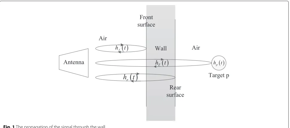
Consider that a region of interest behind a single-layered homogeneous wall is illuminated by a radar system at a certain standoff distance, in which the transmitted signal can be a short pulse with large bandwidth. Since the wall is usually formed of lossy mediums, the wall transmissivity is a function of signal frequency, thus the received radar return cannot be simplified as the superposition of mul-tiple time-shifted and scaled transmitted signalss(t)[25]. As shown in Fig. 1, due to the presence of the wall, the first two echoes in the received return are the reflections from the front and the rear side of the wall and are denoted asyf(t) andyr(t) respectively. Then the received radar
return can be written as [26]
z(t)=yf (t)+yr(t)+
front and the rear interface respectively.hT(t)is the
two-way transmission response of the wall, andhp(t)denotes
Fig. 1The propagation of the signal through the wall
Assuming that the incident angle, the polarization mode, and the standoff distance are all fixed, under this situation,hf (t) can be considered to be only related to the permittivity of the wall since the wall can be viewed as a dielectric slab and, its permittivity can be considered constant within the bandwidth of the signal [27].
As for hr(t) and hT(t), they are associated with
not only the permittivity, but also the wall thickness and the conductivity of the wall. The conductivity refers to the static electric conductivity of the wall and represents the ohmic loss. The imaginary part of the permittivity refers to the AC electric conductivity and represents the polar-ization loss. Since these two parameters are usually small and mainly affect the attenuation of the signal [28], they will not be estimated in this paper. Therefore, the wall parameters that we are focused on are the real part of the permittivity and the thickness.
2.2 The principle of SVR
Suppose that we are given training data
(x1,y1),. . .,(xl,yl)
⊂Rn×R,
where eachxirepresents an input feature vector and has a corresponding target valueyifori=1,. . .,l, wherel
rep-resents the size of the training data set. The basic idea of SVR is to find a functionf (x)that has at mostεdeviation from the actually obtained target values for all the train-ing samples by mapptrain-ing the traintrain-ing data from the input feature space into a higher dimensional space, and mean-while has the capability to approximate future values as accurately as possible [29, 30]. The linear function of SVR takes the formf(x) = ω,x +bwithω ∈ Rn, b ∈ R, where·, ·denotes the dot product inRn.
In standardε-SVR, the value ofωandbcan be deter-mined as the solution of the following convex optimiza-tion problem
whereC > 0 is a regularization constant,ε is the tube radius, andξiandξi∗are the slack variables [31]. The
vec-torωcan be written in terms of data points by solving the dual problem as
whereαiandαi∗are Lagrange multipliers.
For the variableb, it can be computed by applying the Karush-Kuhn-Tucker (KKT) conditions as
b=yi− ω,xi −ε, forαi∈(0,C) b=yi− ω,xi +ε, forαi∗∈(0,C)
(5)
training data fromRnto a higher dimensional space. Thus
where K(xi,x) is the kernel function which enables the inner product in high dimensional space to be performed using low dimensional space data without knowing the transformation. Therefore, SVR can be run readily as long as the kernel function, the penaltyC, and the radius εare chosen appropriately [32].
3 The regular SVR method in WPE
As stated above, through putting the feature vector into the regression function, we can estimate its target value once the regression function is established by SVR. There-fore, the radar returns from diverse walls with different parameters can be collected as the training data, and one can train a regression function for each of the wall param-eters. Then, when we confront a new wall, its parameters can be estimated by taking its radar return into those corresponding regression functions.
Assuming that we have obtained a certain amount of radar returns from different walls, before the train-ing phase, a procedure called feature extraction, which extracts the useful information from the data or trans-forms the data into an appropriate format, should be done to produce the feature vectors. The extracted fea-ture vectors are deemed to be the better representations of the sample data and thus they are more suitable for the regression problem.
The feature vectorvof the radar return extracted by the regular SVR method is produced as follows. The tempo-ral radar returnz(t)can be transformed into frequency domain through
˜
zf=FT {z(t)} (7)
where FT {·} represents the Fourier transform of the associated temporal signal. For N discrete frequencies within the bandwidth, the transformed signalz˜fcan be written in a vector form as
z=z˜f1 ˜zf2 · · · ˜zfN T. (8)
The correlation matrix is defined as=EzzH, where E[·] is the expectation operator, and the superscript ·H indicates the conjugate transpose. In practice, the correla-tion matrixis estimated fromMindependent snapshots of the data vectorz
ˆ
The feature vector is then extracted from the correla-tion matrix [24]. Since the correlacorrela-tion matrix is Hermitian, only the upper triangular half of the matrix is used, and the elements in there are reorganized to form the feature vectorvas follows:
vector will be normalized before using SVR. In this paper, the feature vectors are all normalized with a scale between 0 to 1.
In the regular way, the regression function is trained by SVR for each of the wall parameters independently. Thus there are two training data sets that need to be prepared for the two wall parameters. Let
Bεr = {(v1,εr1),. . .,(vi,εri),. . .,(vl,εrl)}, (11)
wherevidenotes the feature vector of theithtraining
sam-ple and the permittivity εri is the corresponding target
value. Similarly, Let
Bd= {(v1,d1),. . .,(vi,di),. . .,(vl,dl)}. (12)
where di used as target value is the thickness in theith
sample, andlrepresents the number of the total training samples.
Following the instruction about SVR described above, taking the training data sets,Bεr andBd, into SVR
indi-vidually, two regression functions will be obtained. This procedure is termed the training phase in machine learn-ing. Then when a radar return from an unknown wall is received, we put its feature vector into the two regres-sion functions to obtain the estimates of the permittivity and the thickness of the wall, respectively, and this step is called the test phase. For this application, it also can be termed as an estimation phase.
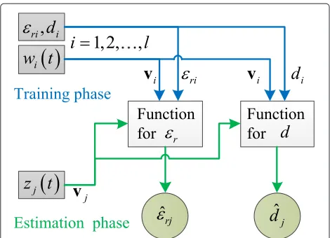
The schematic diagram of the regular SVR method is depicted in Fig. 2.
Fig. 2Diagram of the regular SVR method
4.1 The first stage
It has been pointed out that the samples in training data set may be different from those in the test data set. In this situation, the regular SVR method introduced above can-not provide acceptable estimation results. Therefore, SVR ought to be used in a new way.
Suppose that the training data are given as
{wi(t),εi,di},i=1, 2,. . .,l,
where wi(t) is the radar return from the ith wall with
known parameters(εri,di)and can be written as
wi(t)=yfi(t)+yri(t)+ni(t). (13)
These radar returns are usually collected in a laboratory in advance and do not contain target echoes. During the collection, the incident angle, polarization mode and the standoff distance are all set to be consistent.
Different from the regular SVR method, in order to meet the requirement of our approach, the feature extraction procedure is changed. LetRi(τ)be the cross correlation
function ofwi(t)and the transmitted signals(t)
Ri(τ)=
wi(t+τ)s(t)dt (14)
In training data, since obviously the echoes from the front and the rear sides of the wall are dominant in the received signal, there is no doubt that the two highest peaks inRi(τ)are derived from these two echoes, where
the highest peak represents the echo from the front side while the second highest represents the echo from the rear side. Then, the magnitudes and time delays of these two peaks are extracted and denoted as(β1i,τ1i)and(β2i,τ2i),
respectively.
As stated above, the echo from the front surface is only related to the permittivity of the wall. Therefore, for esti-mating the permittivity, we construct the training data
setBf withvfibeing the feature vectors andεribeing the
target values, where
Based on this training data set, the regression function of the permittivity is trained by SVR and noted as
εr=g
vf
(17)
Then we select the parameters of the wall as another feature vector, that is
vsi=[εri,di]T. (18)
These feature vectors are used to constitute two other training data sets, which are listed as
Bβ2 = {(vs1,β21),. . .,(vsi,β2i),. . .,(vsl,β2l)}. (19)
Bτ2 = {(vs1,τ21),. . .,(vsi,τ2i),. . .,(vsl,τ2l)}. (20) These two sets are used to train the other two regression functions, which are noted as
β2=u(vs) (21)
τ2=v(vs), (22)
respectively. The instrumental variables outputted from these functions will be used to estimate the thickness of the wall later. For now, three regression functions have been trained and established.
4.2 The second stage
For thejth wall that need to be estimated, the received radar return from it is denoted aszj(t), which may contain
the target’s echoes furthermore, that is
zj(t)=yfj(t)+yrj(t)+ P
p=1
ypj(t)+nj(t) (23)
and its cross correlation function with the transmitted signal is given by
Rj(τ)=
zj(t+τ)s(t)dt (24)
InRj, the highest peak still represents the echo from the
time delay of the second highest peak inRjare invalid and
will not be extracted. Letβ1j,τ1j
denote the magnitude and the time delay of the highest peak, which are the only features we extract from Rj(τ). We noticed that only β1 and τ1 can be extracted from both the training and the test data. That is why we select them to constitute the feature vectorvf.
Taking the feature vectorvfj into the functiong(·), we
This is the estimate of the permittivity of thejthwall.
4.3 The third stage
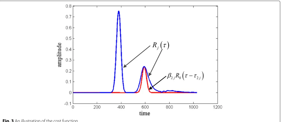
The task of the third stage is to estimate the thickness of the wall. Let us define a cost function at first, which is written as
CF(vs)= R(τ)−β2·R0(τ−τ2)1
= R(τ)−u(vs)·R0(τ−v(vs))1
(26)
where R0(τ) is the normalized autocorrelation function of s(t), ·1 denotes theL1 norm which is the integral of the absolute values of a function. In this equation, the other two regression functionsu(vs)andv(vs)are used to
provide the estimates ofβ2andτ2, respectively.
The motivation of creating this function is to measure the difference between the real echo from the wall rear side and a scaled and shifted transmitted signal, which can be expressed by Fig. 3. If the difference is small, it means that the instrumental variablesβ2andτ2are esti-mated accurately by the regression functions which are associated with the wall parameters, and it further implies that at this moment thst the wall parameters used in the
regression functions approximate to the true wall param-eters. Therefore, the cost function will be a good indicator to the status of the estimation.
For thejthwall, since its estimated permittivity has been
obtained,εˆrj, we define
wheredrepresents the thickness that has not been deter-mined. Substitutingvsj˜ forvsin Eq. (26), we have
CFvsj˜ =Rj(τ)−u
The estimate of the thickness is achieved by minimizing this cost function. Sinceεˆrjis known before, which implies
that the cost function only has one variable, the estimate of the thickness can be expressed as follows,
ˆ
We search the d within a search range and select dˆj
which minimizes the cost function as the estimate of the thickness ofjthwall.
The flow diagram of the proposed approach is depicted in Fig. 4.
Fig. 4Flow diagram of the proposed approach
5 Simulation results
5.1 Description of the simulation
The proposed approach and the regular method are both applied on the data that are generated using FDTD simu-lations. The settings in the simulation are listed as follows:
1. The transmitted radar signal is a Gaussian short-pulse with 1-GHz-frequency bandwidth. The carrier frequency is 1.5 GHz.
2. The transmitting and receiving antennas are placed near each other and both against the wall with a standoff distance of 1 m.
3. Vertical polarization is adopted, and the incident angle is set to zero.
4. The conductivity of the wall is set at 0.01, and the imaginary part of the permittivity of the wall is neglected [33].
5. The SVR part is accomplished using the LIBSVM soft-ware package [34], in whichε-SVR is adopted to perform the regression analysis. By comparing the performances of multiple kernel functions using cross validation on train-ing set, radial basis function (RBF) is selected as the kernel function used in this simulation. The standard form of the RBF Kernel isK(x,y)=exp
−γx−y2
.
6. The parameters (C andγ) that are needed inε-SVR are estimated by the well-knownk-fold cross validation in this simulation, withk = 4. Ink-fold cross-validation, the training data is randomly partitioned intok equally sized subsets. Then inithvalidationi = (1, 2,. . .k), the regression function with the parameters (Ch,γo) is built
usingk −1 subsets as training set. hand oare the hth and theothelements of the parametersCandγ. The per-formance is measured by the mean square error (MSE) on the output from theithsubset that is used as the test
set. The procedure is repeatedktimes, and the average of MSE is calculated. Through searchingCandγ on a user-defined grid, the pair of parameters which provides the best average MSE will be chosen out [35].
5.2 Primary results 1. Training data:
2. Test data (no target):
For the test data, the set of permittivities and the thick-nesses of the walls are composed of 11 equispaced samples within the ranges of [4.5–14.5] and [7.0–27.0 cm], respec-tively. Thus for the test phase, there are also 121 samples in test set. For thejthtest sample, the permittivity and thick-ness of the corresponding wall are denoted asεrj anddj,
respectively.
3. Test data (target withR= 10 cm,Dyj=dj):
In order to test the robustness of the proposed approach when targets exist behind the wall, we generate another test data set, in which the data are collected with the pres-ence of a metal cylinder behind the wall. The cylinder with radius of 10 cm is placed away from the wall with a dis-tanceDyjthat is equal to the current wall thicknessdjin
each sample. Here,Dyjis defined as the distance between
the target’s front surface and the wall’s rear surface in the jthtest sample.
For the proposed SVR method, the training phase and the estimation procedure are carried out in sequence as described above. The pairs of parameters for the three regression functions are obtained by thek−foldmethod, and they are (C = 1180, γ = 3.05× 10⁻⁵) for func-tion g(·), (C = 7130,γ = 0.0068) for u(·), and (C = 65536, γ = 0.0013) for v(·). The search range of d is from 5 to 30 cm with step size of 1 cm through-out the simulation. The simulation results show that such a precision of 1 cm is a good tradeoff between the estimation performance and the computational complexity.
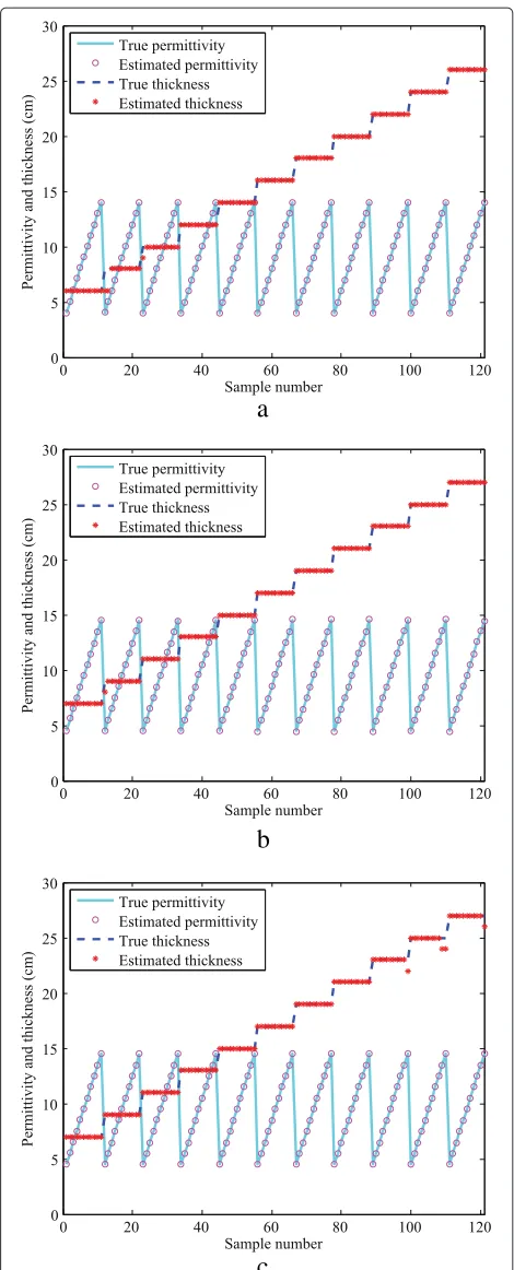
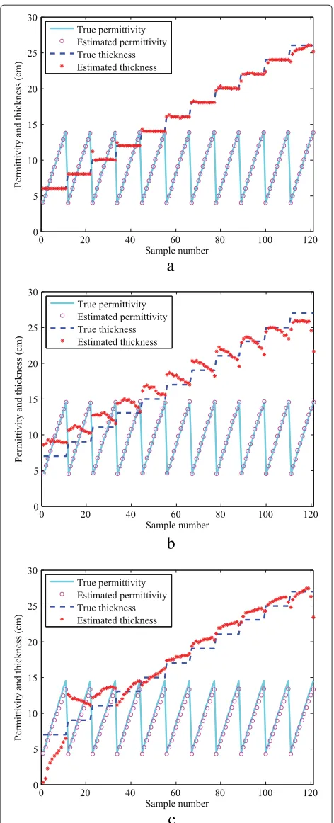
At each run, the proposed approach estimates the per-mittivity and the thickness of the wall for the current test sample. The estimation results of the proposed approach for the samples in training set, the test set without tar-get and the test set with tartar-get, are shown in Fig. 5a, b, c, respectively. In these figures as well as the following illus-trations, the solid lines represent the true permittivities while the circle markers represent the estimated permit-tivities; meanwhile, the dashed lines represent the true thicknesses while the star markers represent the estimated thicknesses.
It is seen that the proposed approach is able to pro-vide the estimates of wall parameters which approximate to the true values, even with the presence of the tar-get. We notice that when the target exists, the estimated thicknesses of those samples which are with large per-mittivities and thickness deviate from their true values a little. This is because when the wall has large permittiv-ity and thickness, the echo from the rear side of the wall will be attenuated and distorted seriously, which means that the echo will have a small amplitude and a long span of time, and thus tends to be more affected by the target echo.
a
b
c
Fig. 5Simulation results obtained by the proposed approach.
For the purpose of comparison, we apply the regular SVR method on those data sets. The pairs of parame-ters for the two regression functions are (C = 3.03,γ = 9.76× 10⁻⁴) for the regression function of permittivity and (C=73.5,γ =0.0118) for the function of thickness. The estimation results are shown in Fig. 6. We see that in Fig. 6a, the estimated results are acceptable, but in Fig. 6b, the test results are not as good as that on the training set. In Fig. 6c, the performance of the regular SVR method deteriorates rapidly since the presence of the target makes the test data different from the training data dramatically.
5.3 Further results
In order to inspect the effect of the presence of the target carefully, more test sets are generated in different scenar-ios and used to measure the performance of the proposed approach.
It is obvious that the closer the target is to the wall, the more seriously the wall echoes will be interfered with the target echo. Hence, we change the distance between the target and the wall in descending order to see the variation of the estimation result. Three test data sets are gener-ated under the situations in which the size of the target is fixed but the the distanceDyjis set to be 1) three times
the current wall thickness for each sample in the first data set; 2) twice the current wall thickness for each sample in the second data set; and 3) 1 cm in the third data set, respectively.
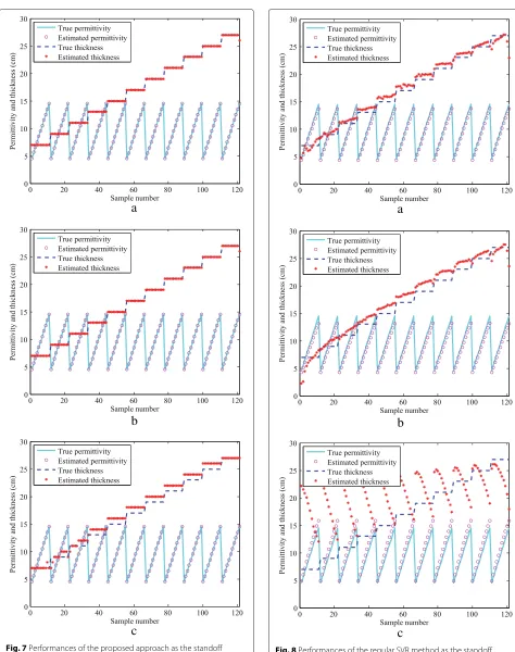
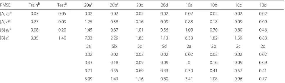
The simulation results based upon these data sets are shown in Fig. 7. As we expected, the estimation results are improved as the target moves far away from the wall. It is seen that in Fig. 7a, b, the estimation results are quite accurate. In Fig. 7c, since the target is very close to the wall, some estimated values of the thickness are larger than the true values. But the errors are relatively small and can be tolerated. In comparison, the estimation results of the regular SVR method is shown in Fig. 8. Similarly, the trend of the performances from Fig. 8a–c also conform to our analysis. However, the performances of the reg-ular SVR method are poorer than that of the proposed approach, especially when the target stands very close to the wall, such as in Fig. 8c. The estimated values of the thickness in it are almost totally wrong.
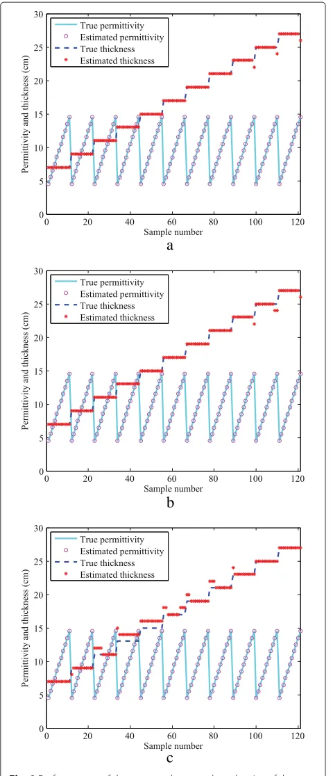
Next, the size of the target is changed in increasing order since it is predictable that a stronger echo from a bigger target will have more serious interference on the echo from the wall. Therefore, three more test data sets are generated under three different scenarios, wherein the distance Dyj is fixed, but the radius of the target is set
to be 1) 2 cm for the first data set; 2) 5 cm for the sec-ond data set, and 3) 20 cm for the third data set. The estimated results from these data sets provided by the pro-posed approach are shown in Fig. 9, which are consistent with our expectation. In Fig. 9c, the estimation errors of
a
b
c
Fig. 6Simulation results obtained by the regular SVR method.
a
b
c
Fig. 7Performances of the proposed approach as the standoff distance changes.aTest data (R=10 cm,Dyj=3×dj);btest data
(R=10 cm,Dyj=2×dj);ctest data (R=10 cm,Dyj=1 cm)
a
b
c
Fig. 8Performances of the regular SVR method as the standoff distance changes.aTest data (R=10 cm,Dyj=3×dj);btest data
a
b
c
Fig. 9Performances of the proposed approach as the size of the target changes.aTest data (R=2 cm,Dyj=dj);btest data (R=5 cm,
Dyj=dj);ctest data (R=20 cm,Dyj=dj)
the thickness are larger than those in Fig. 9a, b, but it is still acceptable. The results obtained by the regular SVR method are given in Fig. 10 for contrast. The performance
a
b
c
Fig. 10Performances of the regular SVR method as the size of the target changes.aTest data (R=2 cm,Dyj=dj);bTest data (R=5 cm,
Dyj=dj);cTest data (R=20 cm,Dyj=dj)
Table 1RMSEs of the estimates
0.02 0.02 0.02 0.02 0.02 0.02 0.02 0.02
0.33 0.18 0.09 0.09 0 0.16 0.09 0.09
0.71 0.55 0.69 0.43 0.30 0.41 0.57 0.41
5.09 1.43 1.16 0.80 3.41 1.08 0.96 0.77
a[A] represents the new proposed approach. [B] represents the regular SVR method. Permittivity and thickness are denoted asε
randd, respectively
b“Train” refers to the training data. “Test” refers to the test data (with no target)
c“20a” represents the test data in which the number “20” indicates that the radius of the target is 20 cm and the letter “a” refers to the distance between the target and the
wall. Here, “a”=1 cm “b”=1×dj. “c”=2×dj. “d”=3×dj
The root-mean-square errors (RMSEs) of the estimated results that can be used to evaluate the performances of the estimation methods in detail are given in Table 1. In addition to the data sets used before, some more data sets are generated and tested, and their estimation results are listed in the table. These simulation results confirm again that the proposed approach can provide satisfactory estimation performance for WPE and prove that the pro-posed approach is superior than the regular SVR method in robustness, accuracy and efficiency.
6 Conclusion
In this paper, SVR is introduced into WPE for the first time. But unlike the typical regression problem, the test data in WPE, i.e., the received radar returns from the walls, are interfered with the target echoes heavily. Against this difficulty, a new approach combining SVR and an optimization procedure is proposed, in which the permittivity is estimated by SVR firstly, and then the thick-ness is achieved by minimizing the cost function based on the estimated permittivity and the instrumental variables provided by SVR also. The numerical experiment results show that the proposed approach can provide accurate estimates of the wall parameters in diverse contexts and outperforms the regular SVR method. In addition, the proposed method has higher computational efficiency since the input feature vectors are in a lower dimen-sion. The training samples needed by this approach can be achieved in advance, thus it is feasible to apply the proposed approach in practice.
Competing interests
The authors declare that they have no competing interests.
Acknowledgements
The work in this paper is supported in part by the General Programs of National Natural Science Foundation of China under Grant No. 61172155 and under Grant No. 61331020.
Received: 25 November 2014 Accepted: 25 June 2015
References
1. F Ahmad, MG Amin, SA Kassam, Synthetic aperture beamformer for imaging through a dielectric wall. Aerosp. Electron. Syst. IEEE Trans.41(1), 271–283 (2005)
2. B Chen, T Jin, B Lu, Z Zhou, Building interior layout reconstruction from through-the-wall radar image using MST-based method. Eurasip J Adv. Signal Process.2014(1), 1–9 (2014)
3. C Clemente, A Balleri, K Woodbridge, JJ Soraghan, Developments in target micro-doppler signatures analysis: Radar imaging, ultrasound and through-the-wall radar. Eurasip J. Adv. Signal Process.2013(1), 1–18 (2013) 4. F Ahmad, MG Amin, T Dogaru, Partially sparse imaging of stationary
indoor scenes. Eurasip J. Adv. Signal Process.2014(1), 1–15 (2014) 5. M Dehmollaian, M Thiel, K Sarabandi, Through-the-wall imaging using
differential SAR. Geoscience Remote Sensing IEEE Trans.47(5), 1289–1296 (2009)
6. T Dogaru, C Le, SAR images of rooms and buildings based on FDTD computer models. Geoscience Remote Sensing IEEE Trans.47(5), 1388–1401 (2009)
7. Y-Z Hu, T-J Li, Z-O Zhou, Use of the location inverse solution to reduce ghost images. Eurasip J. Adv. Signal Process.2010, 1–12 (2010) 8. M Dehmollaian, K Sarabandi, Refocusing through building walls using
synthetic aperture radar. Geoscience Remote Sensing IEEE Trans.46(6), 1589–1599 (2008)
9. R Solimene, FS Prisco, R Pierri, Three-dimensional through-wall imaging under ambiguous wall parameters. Geoscience Remote Sensing IEEE Trans.47(5), 1310–1317 (2009)
10. W Genyuan, MG Amin, Imaging through unknown walls using different standoff distances. Signal Process. IEEE Trans.54(10), 4015–4025 (2006) 11. P Protiva, J Mrkvica, J MacHac, Estimation of wall parameters from
time-delay-only through-wall radar measurements. IEEE Trans. Antennas Propagation.59(11), 4268–4278 (2011)
12. F Ahmad, MG Amin, G Mandapati, Autofocusing of through-the-wall radar imagery under unknown wall characteristics. Image Process. IEEE Trans.16(7), 1785–1795 (2007)
13. X Chen, W Chen, inAntennas and Propagation Society International Symposium (APSURSI), IEEE. A simple method for image autofocusing in through-wall radar imaging (IEEE Piscataway, New Jersey, 2013), pp. 530–531
14. X Li, X Huang, T Jin, Estimation of wall parameters by exploiting correlation of echoes in time domain. Electron. Lett.46(23), 1563–1565 (2010) 15. S Fukuda, H Hirosawa, inGeoscience and Remote Sensing Symposium,
16. Z Qun, JC Principe, Support vector machines for SAR automatic target recognition. Aerospace Electron. Syst. IEEE Trans.37(2), 643–654 (2001) 17. S Kent, NG Kasapoglu, M Kartal, inRadar Conference. RADAR ’08. IEEE. Radar
target classification based on support vector machines and high resolution range profiles (IEEE Piscataway, New Jersey, 2008), pp. 1–6 18. E Pasolli, F Melgani, M Donelli, Automatic analysis of GPR images: A
pattern-recognition approach. Geoscience Remote Sensing IEEE Trans.
47(7), 2206–2217 (2009)
19. T Yajuan, L Xiapu, Y Zijie, inMachine Learning for Signal Processing. Proceedings of the 14th IEEE Signal Processing Society Workshop. Ocean clutter suppression using one-class SVM (IEEE Piscataway, New Jersey, 2004), pp. 559–568
20. K Youngwook, L Hao, Human activity classification based on micro-doppler signatures using a support vector machine. Geoscience Remote Sensing IEEE Trans.47(5), 1328–1337 (2009)
21. W Chun-Hsin, H Jan-Ming, DT Lee, Travel-time prediction with support vector regression. Int. Transport. Syst. IEEE Trans.5(4), 276–281 (2004) 22. D Singh, inGeoscience and Remote Sensing Symposium, IGARSS ’07. IEEE
International. An efficient electromagnetic approach to train the SVM for depth estimation of shallow buried objects with microwave remote sensing data (IEEE Piscataway, New Jersey, 2007), pp. 4961–4964 23. CL Bastard, V Baltazart, X Derobert, W Yide, inGround Penetrating Radar
(GPR), 14th International Conference On. Support vector regression method applied to thin pavement thickness estimation by GPR (IEEE Piscataway, New Jersey, 2012), pp. 349–353
24. CL Bastard, W Yide, V Baltazart, X Derobert, Time delay and permittivity estimation by ground-penetrating radar with support vector regression. Geoscience Remote Sensing Lett. IEEE.11(4), 873–877 (2014) 25. LM Frazier, inEnabling Technologies for Law Enforcement and Security.
Radar surveillance through solid materials (International Society for Optics and Photonics Bellingham, Washington USA, 1997), pp. 139–146 26. TB Gibson, DC Jenn, Prediction and measurement of wall insertion loss.
Antennas Propagation IEEE Trans.47(1), 55–57 (1999)
27. JD Jackson,Classical Electrodynamics, 3rd Edition. (Wiley, New York, 1999) 28. MG Amin,Through-the-Wall Radar Imaging. (CRC Press, Boca Raton,
Florida, 2010)
29. V Vapnik,The Nature of Statistical Learning Theory. (Springer, New York, 1995)
30. H Drucker, CJ Burges, L Kaufman, A Smola, V Vapnik, Support vector regression machines. Adv. Neural Inf. Process. Syst.9, 155–161 (1997) 31. A Smola, B Schölkopf, A tutorial on support vector regression. Stat.
Comput.14(3), 199–222 (2004)
32. V Cherkassky, Y Ma, Practical selection of svm parameters and noise estimation for svm regression. Neural Netw.17(1), 113–126 (2004) 33. A Muqaibel, A Safaai-Jazi, A Bayram, AM Attiya, SM Riad, Ultrawideband
through-the-wall propagation. Microwaves Antennas Propagation IEEE Proc.152(6), 581–588 (2005)
34. C-C Chang, C-J Lin, LIBSVM: A library for support vector machines. ACM Trans. Intell. Syst. Technol.2(3), 1–27 (2011)
35. B Schölkopf, AJ Smola, RC Williamson, PL Bartlett, New support vector algorithms. Neural Comput.12(5), 1207–1245 (2000)
Submit your manuscript to a
journal and benefi t from:
7Convenient online submission 7Rigorous peer review
7Immediate publication on acceptance 7Open access: articles freely available online 7High visibility within the fi eld
7Retaining the copyright to your article