Learning Parsimonious Classification Rules from
Gene Expression Data Using Bayesian Networks with
Local Structure
Jonathan Lyle Lustgarten1,†, Jeya Balaji Balasubramanian2,†,*, Shyam Visweswaran2,3and Vanathi Gopalakrishnan2,3
1 Red Bank Veterinary Hospital / 2051 Briggs Rd, Mt Laurel, NJ 08054, USA; [email protected] 2 Intelligent Systems Program, University of Pittsburgh / 5113 Sennott Square, 210 South Bouquet Street,
Pittsburgh, PA 15260, USA; [email protected] (S.V.); [email protected] (V.G.)
3 Department of Biomedical Informatics, University of Pittsburgh / 5607 Baum Boulevard, Pittsburgh,
PA 15206, USA
* Correspondence: [email protected]; Tel.: +1-412-648-9415 † These authors contributed equally to this work.
Abstract: The comprehensibility of good predictive models learned from high-dimensional gene expression data is attractive because it can lead to biomarker discovery. Several good classifiers provide comparable predictive performance but differ in their abilities to summarize the observed data. We extend a Bayesian Rule Learning (BRL-GSS) algorithm, previously shown to be a significantly better predictor than other classical approaches in this domain. It searches a space of Bayesian networks using a decision tree representation of its parameters with global constraints, and infers a set of IF-THEN rules. The number of parameters and therefore the number of rules are combinatorial to the number of predictor variables in the model. We relax these global constraints to a more generalizable local structure (BRL-LSS). BRL-LSS entails more parsimonious set of rules because it does not have to generate all combinatorial rules. The search space of local structures is much richer than the space of global structures. We design the BRL-LSS with the same worst-case time-complexity as BRL-GSS while exploring a richer and more complex model space. We measure predictive performance using Area Under the ROC curve (AUC) and Accuracy. We measure model parsimony performance by noting the average number of rules and variables needed to describe the observed data. We evaluate the predictive and parsimony performance of BRL-GSS, BRL-LSS and the state-of-the-art C4.5 decision tree algorithm, across 10-fold cross-validation using ten microarray gene-expression diagnostic datasets. In these experiments, we observe that BRL-LSS is similar to BRL-GSS in terms of predictive performance, while generating a much more parsimonious set of rules to explain the same observed data. BRL-LSS also needs fewer variables than C4.5 to explain the data with similar predictive performance. We also conduct a feasibility study to demonstrate the general applicability of our BRL methods on the newer RNA sequencing gene-expression data.
Keywords:rule based models; gene expression data; bayesian networks; parsimony
1. Introduction
Predictive modeling from gene expression data is an important biomedical research task that involves the search for discriminative biomarkers of disease states from a high-dimensional space. Comprehensible models are necessary in order to easily extract the predictive biomarkers from learned classifiers. The number of markers is in the order of several thousand measurements made from much smaller numbers of bio-specimens, often leading to several models that are equally good at the predictive task but differ in their abilities to summarize the observed data.
This BRL algorithm was shown to perform on par or better than three state-of-the-art rule classifiers (Conjunctive Rule Learner[8], RIPPER[9], C4.5[10]) using 24 biomedical datasets. Therein, BRL was shown to outperform even C4.5, which was the best among the other methods. BRL used a global search of the space of possible constrained Bayesian network structures to infer a set of classification rules containing a posterior probability representing their validity. These rules are readily comprehensible and contain biomarkers and their cut-off values that discriminate the class variable.
In this paper, we relax some of the constraints from the BRL search space of global structures by introducing the more generalized local structure search that we call BRL-LSS (Bayesian Rule Learning- Local Structure Search). Henceforth, we refer to the global structure search as BRL-GSS (Bayesian Rule Learning- Global Structure Search) to distinguish it from BRL-LSS. We hypothesize that the more general local structure would lead to more parsimonious rule sets that enhance the comprehensibility of the rule model while maintaining the classification performance.
In this work, we develop an algorithm to perform this local structure search, the BRL-LSS, and evaluate it for parsimony and classification performance using more recently extracted gene expression data from public repositories. We hypothesize that the more generalized representation obtained from the local structure search results in a more parsimonious set of rules that describes the observed data as well as the global structure. Parsimony in the rule set representation contributes towards model comprehensibility by presenting a more concise summary of the observed data. In the Materials and Methods section of this paper, we introduce the BRL algorithm followed by a description of the global and local structure search. We then describe our experimental design to test our hypothesis and observe the results in the subsequent sections.
2. Results and Discussion
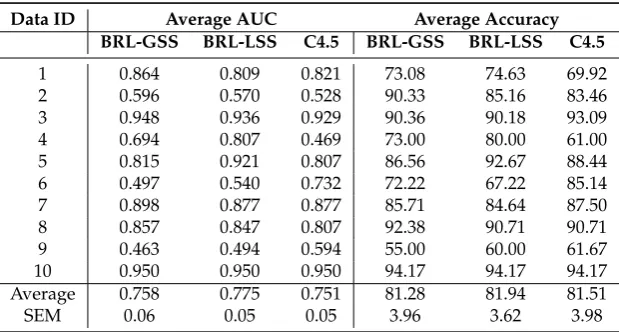
Table 1 shows the summary of the predictive performance of the tested classifiers averaged across the 10 folds of the cross-validation study. For each of the 10 datasets, we report the AUC and the Accuracy. We average the results across the 10 datasets in the bottom of the table. We also provide the standard error of the mean.
Table 1. Predictive performance using the Average and Standard Error of Mean (SEM) of Accuracy and AUC
Data ID Average AUC Average Accuracy
BRL-GSS BRL-LSS C4.5 BRL-GSS BRL-LSS C4.5
1 0.864 0.809 0.821 73.08 74.63 69.92
2 0.596 0.570 0.528 90.33 85.16 83.46
3 0.948 0.936 0.929 90.36 90.18 93.09
4 0.694 0.807 0.469 73.00 80.00 61.00
5 0.815 0.921 0.807 86.56 92.67 88.44
6 0.497 0.540 0.732 72.22 67.22 85.14
7 0.898 0.877 0.877 85.71 84.64 87.50
8 0.857 0.847 0.807 92.38 90.71 90.71
9 0.463 0.494 0.594 55.00 60.00 61.67
10 0.950 0.950 0.950 94.17 94.17 94.17
Average 0.758 0.775 0.751 81.28 81.94 81.51
SEM 0.06 0.05 0.05 3.96 3.62 3.98
In terms of predictive performance each of BRL-GSS, BRL-LSS, and C4.5 appear to be comparable. There seems to be a fractional gain in performance by BRL-LSS with an average AUC of 0.775.
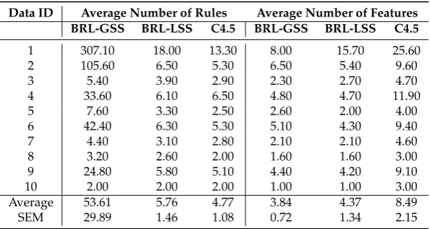
the rule base and the number of variables used. We provide the average and standard error of mean at the bottom of the table.
Table 2. Model Parsimony using the Average and Standard Error of Mean (SEM) of the Number of Rules and Features
Data ID Average Number of Rules Average Number of Features BRL-GSS BRL-LSS C4.5 BRL-GSS BRL-LSS C4.5
1 307.10 18.00 13.30 8.00 15.70 25.60
2 105.60 6.50 5.30 6.50 5.40 9.60
3 5.40 3.90 2.90 2.30 2.70 4.70
4 33.60 6.10 6.50 4.80 4.70 11.90
5 7.60 3.30 2.50 2.60 2.00 4.00
6 42.40 6.30 5.30 5.10 4.30 9.40
7 4.40 3.10 2.80 2.10 2.10 4.60
8 3.20 2.60 2.00 1.60 1.60 3.00
9 24.80 5.80 5.10 4.40 4.20 9.10
10 2.00 2.00 2.00 1.00 1.00 3.00
Average 53.61 5.76 4.77 3.84 4.37 8.49
SEM 29.89 1.46 1.08 0.72 1.34 2.15
The results show that BRL-LSS makes a notably more parsimonious than BRL-GSS. It has fewer average number of rules, 5.76, when compared to BRL-GSS, which needs an average of 53.61 rules to obtain similar performance. The number of rules in BRL-LSS is almost comparable to the state-of-the-art classifier, C4.5, with an average of 4.77 rules. BRL-LSS needs fractionally more number of variables to meet the predictive performance of BRL-GSS. It uses an average of 4.37 variables, while BRL-GSS needs fractionally fewer variables at an average of 3.84. However, C4.5 needed almost twice as many variables (average of 8.49) to obtain the same performance as BRL-LSS.
To summarize, in terms of classification tasks where model parsimony is important (eg. Biomarker discovery) BRL-LSS can be preferred since it selects fewer variables than C4.5, needs fewer rules than BRL-GSS, while having very similar predictive power as the two.
2.1. Case Study
In this sub-section, we analyze the RNA-Seq dataset (KIRC) as described in section 2.2.2. We run BRL-GSS, BRL-LSS, and C4.5 on the KIRC dataset to learn predictive models over 10-fold cross-validation. We observe that the task of differentiating the tumor gene expression from matched normal samples is an easy task for the three algorithms. Each of the tested classifiers were evaluated using the predictive performance metrics (AUC and Accuracy) and the model parsimony metrics (average number of rules and variables used). BRL-LSS emerged as the best predictor with AUC = 0.984 (Accuracy = 99.17%), BRL-GSS as the next best with AUC = 0.975 (Accuracy = 98.69%), and C4.5 achieved an AUC = 0.961 (Accuracy = 98.35%).
We evaluate model parsimony by the average number of rules and variables appearing in models across 10-fold cross-validation. BRL-GSS on average required 10 rules and 2.4 variables. BRL-LSS required fewer rules on average: 7.7 rules with more variables (2.9). C4.5 required the least number of rules (4.3 on average), but needed the largest number of variables on average (7.2 variables) to model the data.
With high performing models, there can be several models that can perform more or less equally well. So, there can be different rule sets learned with BRL (and C4.5) composed of other variables that can match the performance achieved by the greedy best-first search algorithm. We now observe the results we obtained from the greedy best-first algorithms: BRL-GSS and BRL-LSS. The models were learned on the entire KIRC training dataset.
1. IF ((−∞<AQP2≤7.1) AND (−4.9≤C1orf116≤4.0)) THEN (Class =Tumor) Posterior Odds = 476.0, Posterior Probability = 0.998, TP = 475, FP = 0
2. IF ((−∞<AQP2≤7.1) AND (4.6≤C1orf116<∞)) THEN (Class =Tumor) Posterior Odds = 51.0, Posterior Probability = 0.981, TP = 50, FP = 0
3. IF ((7.1≤AQP2≤9.3) AND (−4.9≤C1orf116≤4.0)) THEN (Class =Tumor) Posterior Odds = 9.0, Posterior Probability = 0.9, TP = 8, FP = 0
4. IF ((9.3≤AQP2<∞) AND (−∞<C1orf116≤ −4.9)) THEN (Class =Tumor) Posterior Odds = 1.0, Posterior Probability = 0.5, TP = 0, FP = 0
5. IF ((7.1≤AQP2≤9.3) AND (−∞<C1orf116−4.9)) THEN (Class =Tumor) Posterior Odds = 1.0, Posterior Probability = 0.5, TP = 0, FP = 0
6. IF ((9.3≤AQP2<∞) AND (−4.9≤C1orf116≤4.0)) THEN (Class =Tumor) Posterior Odds = 1.0, Posterior Probability = 0.5, TP = 0, FP = 0
7. IF ((9.3≤AQP2<∞) AND (4.0≤C1orf116≤4.6)) THEN (Class =Tumor) Posterior Odds = 1.0, Posterior Probability = 0.5, TP = 0, FP = 0
8. IF ((−∞<AQP2≤7.1) AND (4.0≤C1orf116≤4.6)) THEN (Class =Tumor) Posterior Odds = 1.0, Posterior Probability = 0.5, TP = 0, FP = 0
9. IF ((7.1≤AQP2≤9.3) AND (4.0≤C1orf116≤4.6)) THEN (Class =Tumor) Posterior Odds = 1.0, Posterior Probability = 0.5, TP = 0, FP = 0
10. IF ((9.3≤AQP2<∞) AND (4.6≤C1orf116<∞)) THEN (Class =Normal) Posterior Odds = 70.0, Posterior Probability = 0.986, TP = 69, FP = 0
11. IF ((−∞<AQP2≤7.1) AND (−∞<C1orf116≤ −4.9)) THEN (Class =Normal) Posterior Odds = 2.0, Posterior Probability = 0.667, TP = 1, FP = 0
12. IF ((7.1≤AQP2≤9.3) AND (4.6≤C1orf116<∞)) THEN (Class =Normal) Posterior Odds = 1.5, Posterior Probability = 0.6, TP = 2, FP = 1
Figure 1.Rule set learned by BRL-GSS on the entire KIRC training data.
takes four discrete values. As expected, this generates twelve rules (four times three). Each rule also shows the number of true positives (TP) and false positives (FP) as computed by the rule on the training dataset. The posterior probability is computed by the smoothed expression–((TP+(TP1)+(+1FP)+1)). The posterior odds are the odds of the rule assigning the predicted class against all other classes–
(TP+1)
(FP+1). We notice that rules 3 through 9 have no evidence assigned from the training dataset. BRL produces rule models that are mutually exclusive and exhaustive. This means that for a given test instance, BRL explains the instance using utmost and at least one rule. The consequence is having rules with no evidence in the training dataset. This was the primary motivation for the development of BRL-LSS that limits the creation of these branches by merging them.
1. IF ((−∞<AIF1L≤9.2) AND (−4.9≤C1orf116≤4.0)) THEN (Class =Tumor) Posterior Odds = 484.0, Posterior Probability = 0.998, TP = 483, FP = 0
2. IF ((−∞<AIF1L≤9.2) AND (4.6≤C1orf116<∞)) THEN (Class =Tumor) Posterior Odds = 45.0, Posterior Probability = 0.978, TP = 44, FP = 0
3. IF ((9.2≤AIF1L<∞) AND (−∞<AMPH≤0.6)) THEN (Class =Tumor) Posterior Odds = 8.0, Posterior Probability = 0.889, TP = 7, FP = 0
4. IF ((−∞<AIF1L≤9.2) AND (4.0≤C1orf116≤4.6)) THEN (Class =Tumor) Posterior Odds = 1.0, Posterior Probability = 0.5, TP = 0, FP = 0
5. IF ((9.2≤AIF1L<∞) AND (1.6≤AMPH<∞)) THEN (Class =Normal) Posterior Odds = 60.0, Posterior Probability = 0.984, TP = 59, FP = 0
6. IF ((9.2≤AIF1L<∞) AND (0.6≤AMPH≤1.6)) THEN (Class =Normal) Posterior Odds = 13.0, Posterior Probability = 0.929, TP = 12, FP = 0
7. IF ((−∞<AIF1L<9.2) AND (−∞<C1orf116≤ −4.9)) THEN (Class =Normal) Posterior Odds = 2.0, Posterior Probability = 0.667, TP = 1, FP = 0
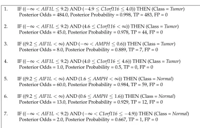
Figure 2.Rule set learned by BRL-LSS on the entire KIRC training data.
rules(two times three times four) that is largely composed of rules with no evidence in the training dataset. Using BRL-LSS, we manage to maintain the property of the rule set being mutually exclusive and exhaustive while achieving parsimony. The BRL-LSS rule set only requires 7 rules to describe the training data, while needing 3 variables to do so. We still end up with rules with no evidence (rule 4) but they are much fewer.
The purpose of this case study was to demonstrate the application of BRL-GSS and BRL-LSS in data from RNA-Seq technology. A complete data analysis of the KIRC dataset would involve further exploratory data analysis and examination of multiple rule sets to explain different hypothesis. Such thorough analysis of this dataset is beyond the scope of this paper.
3. Materials and Methods
3.1. Bayesian Rule Learning
A classifier is learned from gene expression data to explain disease states from historical data. The variable of interest that is predicted is called the target variable(or simply thetarget), and the variables used for prediction are called thepredictor variables(or simplyfeatures).
Rule-based classifiers are a class of easily comprehensible supervised machine learning models that explain the distribution of the target, in the observed data, using a set of IF-THEN rules described using predictor variables. The ’IF’ part of the rule specifies a condition, also known as the rule antecedent, which if met, fires the ’THEN’ part of the rule, known as therule consequent. The rule consequent makes a decision on the class label, given the value assignments of the predictor variables met by the rule antecedent. A set of rules is called arule base, which is a type of knowledge base. The C4.5 algorithm learns a decision tree, where each path in the decision tree (from root of the tree to each leaf) can be interpreted as a rule. Here the variables selected in the path compose the rule antecedents as a conjunctions of predictive variable and value assignment to those variables. We infer a rule consequent based on the distribution of instances over the target that match this rule antecedent.
parameters [11]. The graphical structure consists of a directed acyclic graph. Here, the nodes represent variables and variables are related to each other by directed arcs that do not form any directed cycles. When there is a directed arc from node Ato node B, nodeBis said to be the child node, and nodeAis said to be theparent node. A probability distribution is associated with each node, X, in the graphical structure given the state of its parent nodes,P(X|Pa(X)), wherePa(X)represents the different discrete value assignments of the parents of nodeX. This probability distribution is generally called a conditional probability distribution (CPD). For discrete-valued random variables, the CPD can be represented in form of a table called conditional probability table (CPT). Furthermore, any CPT can be represented as a rule base. Here, we consider only the CPT for the target variable. Each possible value assignments of the parents represent a different rule in the rule base. The evidence in form of the distribution of instances, for each target value, in the training data helps infer the rule consequent. The resulting rule base consists of rules that are mutually exclusive and exhaustive. In other words, at least one rule from the rule base matches a given instance and only one rule matches that instance.
We learn a BN from a training dataset using a heuristic search of the decision tree that results from the CPT described above. We evaluate how likely our learned BN generated the observed data using the Bayesian score (the K2 metric [12]). We demonstrated this process in our previous work [7]. Decision trees are popular compact representations of the CPT of a node in a BN. Most of BN literature is dedicated to learning global independence constraints in the domain. The global constraints only capture the dependent and independent variables that are parents to the node in the graphical representation. The number of parameters needed to describe the CPT is the number of joint assignments for the different parent variables of the node. The size of this CPT grows combinatorially to the number of parents of the node. As an example, let us consider a node representing a disease state. Let there be 10 genes (henceforth when we mention gene as a variable we are referring to its expression) that lead to the change of disease state. Let each gene take two discrete values (UP: up-regulated, DOWN: down-regulated). This would require 210=1024 parameters to be represented by the CPT. Consequently our rule base has 1024 rules, one for each value assignment of the parent variables. Biomedical research, especially gene expression data rarely have enough training data to provide sufficient evidence to make class inference from the 1024 rules in our example scenario. It is therefore important to come up with a more efficient representation of the CPT.
3.1.1. Bayesian Rule Learning- Global Structure Search (BRL-GSS)
We constrained our model to only those models with variables being a direct parent of the target variable. BRL uses breadth-first marker propagation (BFMP) for this algorithm, which provides significant speed up since database look-up is an expensive operation [13]. BFMP [13] permits bi-directional look-up using vectors of pointers by linking a sample to its respective variable-values, and the variable value to those samples that have it. It enables efficient generation of counts of matches for all possible specializations of a rule using these pointers.
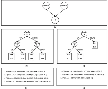
Figure 3. Bayesian Rule Learning: (a) Bayesian Network for targetDand predictor variables Gene Aand geneB. (b)BRL-GSSCPT represented as a decision tree withglobalconstraints. (c)BRL-GSS Decision tree represented as a BRL rule base. (d)BRL-LSSCPT represented as a decision tree with localconstraints. (e)BRL-LSSDecision tree represented as a BRL rule base.
Figure3c depicts a decision tree represented as a rule base. The rule antecedent (IF part) contains a conjunction of predictor variable assignments as shown in the path of the decision tree. The rule consequent is the conditional probability distribution over the target values (in square brackets) followed by the the distribution of the instances from the training data for each target value that match the rule antecedent. In rule 1, we see the evidence to be (50, 5) where there are 50 instances in the training dataset that matches the rule antecedent that have valueD=true. There are only 5 instances that matches the rule antecedent that have valueD= f alse. They are then smoothed with a factorα, set to 1 as a default. This simplifies the posterior odds to the ratio of(TP+α)/(FP+α), where TP is the number of true positives for the rule (where both the antecedent and consequent match with the test instance) and FP is the number of false positives (antecedent matches, but consequent does not match the test instance).
During prediction the class is determined by simply the higher conditional probability. In our example, sinceD=truehas a probability of 0.89, the prediction for a test case that matches this rule antecedent isD=true. If there is a tie, by default the value of the majority class is the prediction.
BRL1000version of the algorithm and rename it to BRL-GSS to be consistent with nomenclature for the local structure search algorithm we present in the next section. The worst-case time-complexity of BRL-GSS, for a dataset withnvariables andminstances, where each variableihasridiscrete values andr =maxri, isO(n2mr). If we constrain the maximum number of discrete values that a variable can take on (for example, assume all variables are binary-valued), then the time-complexity reduces toO(n2m).
3.1.2. Bayesian Rule Learning- Local Structure Search (BRL-LSS)
We adapted the method developed by [14] which can be used for developing an entire global network based on local structure. In Figure 3a, we see the same BN with two parents as the one we saw in BRL-GSS. Figure3d, shows the local decision tree structure. In Figure3, we saw that the distribution of the target, when Gene A = DOW N is the same regardless of the value of Gene B. To be precise,P(D|GeneA=DOW N,GeneB=UP) =P(D|GeneA= DOW N,GeneB=DOW N) = [0.34, 0.66]. The more general representation in Figure3d, merges the two redundant leaves to provide a single leaf. As a result Figure3e, reduces the number of rules to 3 down from 4. So, Figure3e is said to be a more parsimonious representation of the data when compared to Figure3c.
Next, we describe our algorithmic implementation to learn local decision trees as seen in Figure 3d. At a high level, our algorithm initializes a model with a single variable (gene) node as the root. For each unique variable in the dataset, there can be a unique root at the decision tree. A leaf in the initial model represents a specific value assignment of the root variable. By observing the classes of instances in the dataset that match this variable value assignment, we infer the likely class of an instance that would match this variable value assignment. To evaluate the overall model, we use the Bayesian Score to evaluate the likelihood that this model generated the observed data. The algorithm then iteratively explores further specialized models by adding other variables as nodes to one of the leaves of the decision tree. The model is then re-evaluated using the Bayesian Score. The model space here is huge atO(n!). Our algorithm adds some greedy constraints to bring the space down. In the following paragraphs, we specify how we constrain the search.
Algorithm1is the pseudocode of the local structure search module in the BRL. This algorithm takes as input, the dataDand two parametersmaxConjandbeamWidthsimilar to BRL-GSS. We also used the heuristic of maximum number of parents (maxConj) to prevent overspecialization as well as to reduce the running time (default is set to 8 variables per path). ThebeamWidthparameter is the size of the priority queue (beam) that limits the number of BNs that the search algorithm stores in memory at a given step of the search. This beam sorts the BNs in reducing order of their Bayesian score. Line 2 initializes this beam withsingleton models. These BNs have a single child and a single parent. The child is fixed to be the target. The parent is set iteratively to all the predictor variables in the training dataD. During the search, this initial parent variable is set as the root node of the tree. A variable node is split in two ways— 1) Binary split and 2) Complete split. In binary split the variable is split into two values. If the variable has more than two discrete values (say|v|), the binary split creates(|v2|)different combinations of local decision trees. The complete split generates|v|different paths, one for each discrete value of the variable.
Lines 18 through 21 check if the specialization process led to an improvement (better Bayesian score) to the model it started with. If the score improves, the new model is queued for further specialization in the subsequent iterations of the search algorithm.
Finally, in line 23 the best model seen during the search so far is returned by the search algorithm. This best-first search algorithm uses a beam to search through a space of local structured CPTs of BNs. As described in Figure3e, BRL interprets this decision tree as a rule base.
Algorithm 1:BAYESIANLOCALSTRUCTURESEARCH
Input : Data (D), maximum number of unique variables in one model (maxConj), number of models in search memory (beamWidth).
Output: A Priority Queue f inalwithbeamWidthmodels with the highest Bayesian Scores saved during the search.
1 Initialize a Priority Queuef inalwith capacitybeamWidth;
/* Create a Priority Queue of beamWidth Bayesian networks, each with
one child (target variable) and one parent variable with each
predictor variable in D. */
2 modelsToDevelop←Initialize-Models(D,beamWidth); 3 whilemodelsToDevelop6=∅do
4 Initialize a Priority Queuetemp;
5 foreachModel Mcurr∈modelsToDevelopdo 6 AddMcurrto f inal;
7 if|Mcurr.parents|<maxConjANDMcurr.unexplored6=∅then 8 foreachVariable v∈Mcurr.unexploreddo
9 Mvbest←Mcurr;
10 foreachLeaf f ∈ Mvbest.leavesdo
11 ifv∈/ f.paththen
/* Splits variable v to the number of discrete
values it takes. */
12 Mtemp←Complete-Split(Mvbest,f,v);
13 ifMtemp.score> Mvbest.scorethen
14 Mvbest←Mtemp;
/* Splits variable v as a binary variable, by |v|
choose 2 different splits and returning the one
with the best Bayesian Score. */
15 Mtemp←Binary-Split(Mbestv ,f,v);
16 ifMtemp.score> Mvbest.scorethen
17 Mvbest←Mtemp;
18 ifMvbest.score>Mcurr.scorethen
19 Mvbest.explored←Mbestv .explored+v; 20 Mvbest.unexplored←Mvbest.unexplored−v;
21 AddMbestv totemp;
22 modelsToDevelop←temp 23 return f inal;
can take, the complexity reduces toO(n2m). As a result, with BRL-LSS we now explore a much richer space of models with the same time-complexity as BRL-GSS.
3.2. Experimental Design
For each biomedical dataset, we split the data into train and test set using cross-validation split. BRL-GSS and BRL-LSS require discrete data so, the training dataset is discretized. After learning the discretization scheme for each of the features from the training data, we apply the discretization scheme on those features in the test dataset. Finally, we learn a rule model from our different algorithms on the training data. We use this model to predict on the test data and we evaluate our performance. The detailed description on the cross-validation design, discretization method, classification algorithms, and performance metrics used for evaluation is described below.
3.2.1. Classification Algorithms
We test three algorithms in the modeling step of the experimental design framework, to generate our rule models— 1) TheBRL-GSS, which was the significantly best model from our previous study [7] comparing other state-of-the-art rule models; 2)BRL-LSS, which is our proposed method in this paper with a promise on model parsimony; and finally 3) We have shown previously [7] that C4.5 outperforms other readily available rule learners, and therefore for the purposes of comparison in this paper, we consider C4.5 as state-of-the-art. Decision trees can be translated into a rule base by inferring a rule from each path in the decision tree. C4.5[10] is the most popular decision tree based method. It was an extension to an earlier ID3 algorithm.
Both the BRL methods take in two parameters—maxConj, maximum number of features used in the Bayesian Network model, andbeamWidth, maximum number of models stored in the search memory. For both BRL-GSS and BRL-LSS, we setmaxConj =8, andbeamWidth=1000. These were arbitrary choices that we use as defaults for the BRL models. The C4.5 also uses its default parameters as set by Weka.
3.2.2. Dataset
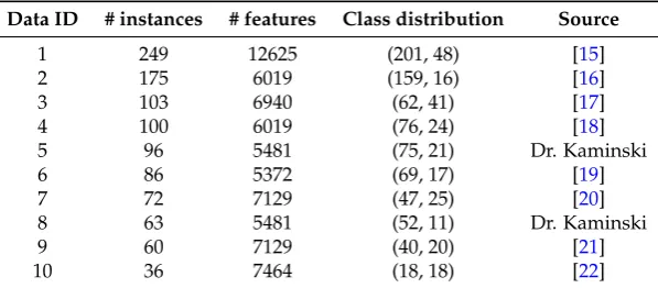
We run our experiments on 10 binary class, high-throughput, biomedical data. Each of the 10 datasets chosen here represent a cancer diagnostic problem of distinguishing cancer patients from normal patients using their gene expression profile. The gene expression data is generated from high-throughput microarray technology. Table3shows the dataset dimensions and sources for the 10 datasets.
Table 3.The 10 datasets used in our experiments (sorted by the number of instances). The columns indicate the data ID number, number of instances, number of features, the class label distribution among the instances, and the source of the data.
Data ID # instances # features Class distribution Source
1 249 12625 (201, 48) [15]
2 175 6019 (159, 16) [16]
3 103 6940 (62, 41) [17]
4 100 6019 (76, 24) [18]
5 96 5481 (75, 21) Dr. Kaminski
6 86 5372 (69, 17) [19]
7 72 7129 (47, 25) [20]
8 63 5481 (52, 11) Dr. Kaminski
9 60 7129 (40, 20) [21]
10 36 7464 (18, 18) [22]
(RNA-Seq) technology for gene expression. We obtain Illumina HiSeq 2000, RNA-Seq Version 2, normalized, gene expression data of patients with Kidney Renal Clear Cell Carcinoma (KIRC), processed using the RNA-Seq Expectation Maximization (RSEM) pipeline from The Cancer Genome Atlas (TCGA)[23]. The samples are primary nephrectomy specimens obtained from patients with histologically confirmed clear cell renal cell carcinoma and the specimens conform to the requirements for genomic study by TCGA. We develop a model to differentiate the gene expression in tumor samples from matched normal samples (normal samples from patient with the tumor). This KIRC dataset has 606 samples (534 tumor, 72 normal) and 20531 mapped genes.
We pre-process the KIRC dataset by removing genes with sparse expression (more than 50% of the samples have value 0). We are left with 17694 genes. As recommended in RNA-Seq analysis literature [24], we use Limma’s voom transformation[25] to remove heteroscedasticity from RNA-Seq count data and to be unaffected by outliers in the data. In this case study described in the results section 3.1, we demonstrate the feasibility of our rule learning methods in analyzing RNA-Seq data.
As described in the experimental design framework, our datasets need to be discretized for applying our algorithms. All the biomedical datasets in Table3contain continuous measurements of the markers. Each training fold of data is discretized using the efficient Bayesian discretization method (EBD) [26] with a default parameter, λ = 0.5, which controls the expected number of cut-points for each variable in the dataset.
3.2.3. Evaluation
For each of the 10 datasets, we performed a 10-fold stratified cross-validation for sampling from a dataset. We measure each performance metric (described below) for each fold in the cross-validation and then average that metric across the 10 folds to get an estimate of that performance metric.
We measure 4 performance metrics. We use 2 metrics to evaluate the classifier predictive performance, and another 2 to evaluate model parsimony. The first metric for classifier predictive performance is theArea Under the Receiver Operator Characteristics Curve(AUC). It indicates the class discrimination ability of the algorithm for each dataset. It ranges from 0.0 to 1.0. Higher value indicates a better predictive classifier. The second metric for classifier performance isAccuracy, given as a percentage. Again higher value indicates a better predictor.
The first parsimony metric is theNumber of Rules. All the algorithms tested have rule bases that are mutually exclusive and exhaustive. This means that each instance in the dataset is covered by at least one rule, and exactly one rule. A small number of rules in the rule base indicates greater coverage by individual rules. The coverage of a rule is the fraction of the instances in the training data that satisfies the antecedent of the rule. A large number of rules indicates that each rule have small coverage, and as a result lesser evidence. A small number here is attractive because a parsimonious model with few rules to describe all the observed data indicates generalized rules with stronger evidence per rule. The second parsimony metric is theNumber of Variables. Typically in a biomarker discover task that involves a high-dimensional gene expression data, we would like fewer variables to describe the observed data. This is because the validation of those markers is time consuming and expensive. Having fewer variables to verify is appealing in this domain. So, we prefer fewer number of variables that gives us the best predictor.
4. Future Work
An important problem in genomics is the classification of a SNP as either neutral or deleterious. Deleterious SNPs can disrupt functional sites in a protein and can cause several disorders. SNPdryad[28] is one such classifier that uses only orthologous protein sequences to derive features (Sequence Conservation Profile) that assist in this classification task. In addition to the Sequence Conservation Profile, they use other features like the physiochemical property of amino acids, the functional annotation of the region with the SNP, number of sequences in the multiple sequence alignment, and the number of distinct amino acids for the classification task. They compare 10 different classifiers for the task and report excellent predictive performance using Random Forests. However, they do not explore any classifier that offers readily interpretable descriptive statistics. We propose to explore this problem using the BRL system, since it readily offers descriptive statistics in form of rule sets. It would be interesting to learn which features lead to deleterious non-synonymous human SNPs.
Another problem of interest is thein silicoevaluation of target sites for the CRISPR/Cas9 system. CCTop[29] is an experimentally validated tool that is used to select and evaluate targeting site for the CRISPR/Cas9 system. CCTop evaluates target sites in a genome by using a score derived from the likelihood of the stability of the heteroduplex (formed from the single guide RNA and the DNA) and the proximity of an exon to the target. BRL system can be used to learn rules that indicate a good target site for the CRISPR/Cas9 system. The classifiers in the BRL system are composed of rules, each with a posterior probability indicating the uncertainty in the validity of the rule. This probability score can be used to rank the target sites. In addition, it would be interesting to explore other candidate variables to improve the performance of the rule sets.
5. Conclusions
In this paper, we presented extensions to the BRL-GSS by relaxing the constraints on the decision tree representation using local structures of the conditional probability table of the learned Bayesian network. This led to the creation of BRL-LSS that explores a richer and more complex model space while maintaining the worst-case time-complexity with BRL-GSS. BRL-LSS is now incorporated as part of the BRL system, which is provided in the Supplementary materials. This system can be used for predictive modeling of any quantitative datasets, even though it has been developed primarily for the analysis of biomedical data. The advantages of this system over state-of-the-art machine learning classifiers include: 1) comprehensibility and ease in extracting discriminative variables/ biomarkers from interpretable rules, and 2) parsimonious models with comparable predictive performance, and 3) the ability to handle discretization of high-dimensional biomedical datasets using simple command line parameters integrated into the BRL system. We hope that BRL system will find applications in other challenging domains especially the ones with high-dimensional data.
Acknowledgments: We wish to thank all our anonymous reviewers for helping significantly improve our manuscript. An important contribution from our anonymous reviewers includes providing us with specific directions for our research summarized in the Future Work section of this manuscript. Research reported in this publication was supported by the National Library of Medicine of the National Institutes of Health under award numbers T15LM007059 and R01LM012095, and by the National Institute of General Medical Sciences of the National Institutes of Health under award number R01GM100387. The content is solely the responsibility of the authors and does not necessarily represent the official views of the National Institutes of Health.
Author Contributions: J.L.L and J.B.B developed the BRL system and tested the ideas in this paper. S.V and V.G conceived of the study and guided the development of the algorithms and experiments for this paper. J.B.B produced the draft of the paper and circulated it to all authors. All authors read, revised, and approved the final version for submission.
References
1. Bigbee, W.L.; Gopalakrishnan, V.; Weissfeld, J.L.; Wilson, D.O.; Dacic, S.; Lokshin, A.E.; Siegfried, J.M. A multiplexed serum biomarker immunoassay panel discriminates clinical lung cancer patients from high-risk individuals found to be cancer-free by CT screening.Journal of Thoracic Oncology2012,7, 698–708. 2. Ganchev, P.; Malehorn, D.; Bigbee, W.L.; Gopalakrishnan, V. Transfer learning of classification rules for biomarker discovery and verification from molecular profiling studies. Journal of biomedical informatics 2011,44, S17–S23.
3. Gopalakrishnan, V.; Ganchev, P.; Ranganathan, S.; Bowser, R. Rule learning for disease-specific biomarker discovery from clinical proteomic mass spectra. International Workshop on Data Mining for Biomedical Applications. Springer, 2006, pp. 93–105.
4. Ranganathan, S.; Williams, E.; Ganchev, P.; Gopalakrishnan, V.; Lacomis, D.; Urbinelli, L.; Newhall, K.; Cudkowicz, M.E.; Brown, R.H.; Bowser, R. Proteomic profiling of cerebrospinal fluid identifies biomarkers for amyotrophic lateral sclerosis. Journal of neurochemistry2005,95, 1461–1471.
5. Ryberg, H.; An, J.; Darko, S.; Lustgarten, J.L.; Jaffa, M.; Gopalakrishnan, V.; Lacomis, D.; Cudkowicz, M.; Bowser, R. Discovery and verification of amyotrophic lateral sclerosis biomarkers by proteomics. Muscle & nerve2010,42, 104–111.
6. Gopalakrishnan, V.; Williams, E.; Ranganathan, S.; Bowser, R.; Cudkowic, M.E.; Novelli, M.; Lattazi, W.; Gambotto, A.; Day, B.W. Proteomic data mining challenges in identification of disease-specific biomarkers from variable resolution mass spectra. Proceedings of SIAM Bioinformatics Workshop. FL: Lake Buena Vista, 2004, Vol. 10.
7. Gopalakrishnan, V.; Lustgarten, J.L.; Visweswaran, S.; Cooper, G.F. Bayesian rule learning for biomedical data mining.Bioinformatics2010,26, 668–675.
8. Fürnkranz, J.; Widmer, G. Incremental reduced error pruning. Proceedings of the 11th International Conference on Machine Learning (ML-94), 1994, pp. 70–77.
9. Cohen, W.W. Fast effective rule induction. Proceedings of the twelfth international conference on machine learning, 1995, pp. 115–123.
10. Quinlan, J.R.C4. 5: programs for machine learning; Elsevier, 2014. 11. Neapolitan, R.E.; others. Learning bayesian networks2004.
12. Cooper, G.F.; Herskovits, E. A Bayesian method for the induction of probabilistic networks from data. Machine learning1992,9, 309–347.
13. Aronis, J.M.; Provost, F.J. Increasing the Efficiency of Data Mining Algorithms with Breadth-First Marker Propagation. KDD, 1997, pp. 119–122.
14. Friedman, N.; Goldszmidt, M. Learning Bayesian networks with local structure. InLearning in graphical models; Springer, 1998; pp. 421–459.
15. Yeoh, E.J.; Ross, M.E.; Shurtleff, S.A.; Williams, W.K.; Patel, D.; Mahfouz, R.; Behm, F.G.; Raimondi, S.C.; Relling, M.V.; Patel, A.; others. Classification, subtype discovery, and prediction of outcome in pediatric acute lymphoblastic leukemia by gene expression profiling. Cancer cell2002,1, 133–143.
16. Gravendeel, L.A.; Kouwenhoven, M.C.; Gevaert, O.; de Rooi, J.J.; Stubbs, A.P.; Duijm, J.E.; Daemen, A.; Bleeker, F.E.; Bralten, L.B.; Kloosterhof, N.K.; others. Intrinsic gene expression profiles of gliomas are a better predictor of survival than histology.Cancer research2009,69, 9065–9072.
17. Lapointe, J.; Li, C.; Higgins, J.P.; Van De Rijn, M.; Bair, E.; Montgomery, K.; Ferrari, M.; Egevad, L.; Rayford, W.; Bergerheim, U.; others. Gene expression profiling identifies clinically relevant subtypes of prostate cancer.Proceedings of the National Academy of Sciences of the United States of America2004,101, 811–816. 18. Phillips, H.S.; Kharbanda, S.; Chen, R.; Forrest, W.F.; Soriano, R.H.; Wu, T.D.; Misra, A.; Nigro, J.M.;
Colman, H.; Soroceanu, L.; others. Molecular subclasses of high-grade glioma predict prognosis, delineate a pattern of disease progression, and resemble stages in neurogenesis. Cancer cell2006,9, 157–173. 19. Beer, D.G.; Kardia, S.L.; Huang, C.C.; Giordano, T.J.; Levin, A.M.; Misek, D.E.; Lin, L.; Chen, G.;
Gharib, T.G.; Thomas, D.G.; others. Gene-expression profiles predict survival of patients with lung adenocarcinoma. Nature medicine2002,8, 816–824.
21. Iizuka, N.; Oka, M.; Yamada-Okabe, H.; Nishida, M.; Maeda, Y.; Mori, N.; Takao, T.; Tamesa, T.; Tangoku, A.; Tabuchi, H.; others. Oligonucleotide microarray for prediction of early intrahepatic recurrence of hepatocellular carcinoma after curative resection. The lancet2003,361, 923–929.
22. Hedenfalk, I.; Duggan, D.; Chen, Y.; Radmacher, M.; Bittner, M.; Simon, R.; Meltzer, P.; Gusterson, B.; Esteller, M.; Raffeld, M.; others. Gene-expression profiles in hereditary breast cancer. New England Journal of Medicine2001,344, 539–548.
23. Network, C.G.A.R.; others. Comprehensive molecular characterization of clear cell renal cell carcinoma. Nature2013,499, 43–49.
24. Soneson, C.; Delorenzi, M. A comparison of methods for differential expression analysis of RNA-seq data. BMC bioinformatics2013,14, 1.
25. Law, C.W.; Chen, Y.; Shi, W.; Smyth, G.K. Voom: precision weights unlock linear model analysis tools for RNA-seq read counts.Genome biology2014,15, 1.
26. Lustgarten, J.L.; Visweswaran, S.; Gopalakrishnan, V.; Cooper, G.F. Application of an efficient Bayesian discretization method to biomedical data. BMC bioinformatics2011,12, 1.
27. Balasubramanian, J.B.; Visweswaran, S.; Cooper, G.F.; Gopalakrishnan, V. Selective Model Averaging with Bayesian Rule Learning for Predictive Biomedicine.AMIA Summits on Translational Science Proceedings2014, 2014, 17.
28. Wong, K.C.; Zhang, Z. SNPdryad: predicting deleterious non-synonymous human SNPs using only orthologous protein sequences. Bioinformatics2014,30, 1112–1119.
29. Stemmer, M.; Thumberger, T.; del Sol Keyer, M.; Wittbrodt, J.; Mateo, J.L. CCTop: an intuitive, flexible and reliable CRISPR/Cas9 target prediction tool. PloS one2015,10, e0124633.
c