Comparative Study of Various Approximations to the Covariance Matrix in Template Attacks

(1)

to the Covariance Matrix in Template Attacks

Mathias Wagner, Yongbo Hu, Chen Zhang, Yeyang Zheng

NXP Semiconductors

Abstract. Template attacks have been shown to be among the strongest attacks when it comes to side–channel attacks. An essential ingredient there is to calculate the inverse of a covariance matrix. In this paper we make a comparative study of the effectiveness of some 24 different variants of template attacks based on different approximations of this covariance matrix. As an example, we have chosen a recent smart card where the plain text, cipher text, as well as the key leak strongly. Some of the more commonly chosen approximations to the covariance matrix turn out to be not very effective, whilst others are.

1 Introduction

Side–channel attacks have by now a very long history [1–3], and also the par-ticular variant of template attacks [5–9] has been studied for quite some years. A critical piece in all these analysis is the calculation of a covariance matrix, and possibly approximations to it. The majority of the work published so far either uses the original definition, a simple average over all covariances, or some linearization thereof.

(2)

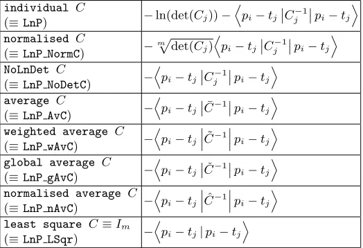
Table 1. Non–linear, non–differential template attack variants with generic names. Variablestjandpirefer to the templates / profiles created in the profiling respectively the Exploitation Phase, and m is the number of Points of Interest (POI). Averages over the entire respective data sets are denoted as ¯tand ¯p, respectively. The various averages of the covariance matrix, like ¯C, ˜C, and ˆC are defined in Eqs. (4–6).

individual C

(≡LnP) −ln(det(Cj))−

D

pi−tjC

−1

j pi−tj

E

normalised C

(≡LnP NormC) −

mp

det(Cj)Dpi−tj C

−1

j pi−tj

E

NoLnDet C

(≡LnP NoDetC) −

D

pi−tjC

−1

j pi−tj

E

average C

(≡LnP AvC) −

D

pi−tjC¯

−1 pi−tj

E

weighted average C

(≡LnP wAvC) −

D pi−tj

˜

C−1 pi−tj

E

global average C

(≡LnP gAvC) −

D

pi−tjCˇ−1 pi−tj

E

normalised average C

(≡LnP nAvC) −

D pi−tj

ˆ

C−1 pi−tj

E

least square C≡Im

(≡LnP LSqr) −

D

pi−tj|pi−tjE

In this paper we will address an improvement over what is currently state of the art for template attacks with regards to the evaluation and use of the covariance matrix.

In Sec. 2 we will discuss various approximations to the probability density function of the multivariate normal distribution typically used in template at-tacks. It will be seen that it is worthwhile evaluating all these approximations, since they can yield widely different results, depending on the situation, but every time consistently so. Since the attacker can study the strengths of these approximations in the Profiling Phase, we have to assume that the attacker will pick the strongest one for the actual attack.

Following a recent finding [10], in Sec. 3 these approximations are applied to the analysis of the DES hardware coprocessor of a recent smart card, where leakage is found for plain text, cipher text, as well as key in the form of P[i]⊕

P[i+ 4], whereP[i] refers to thei–th byte of the plain text, andC[i]⊕C[i+ 4], as well asK[i]⊕K[i+ 4],i= 0...3.

2 Approximations to the Probability Function

The starting point is the standard definition of the template–matching proba-bilityPij, which except for constant terms that neither depend on the template

(3)

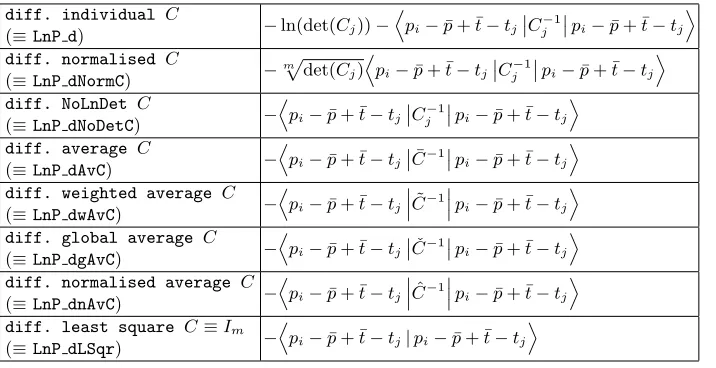
Table 2.Differential non–linear template attack variants.

diff. individual C

(≡LnP d) −ln(det(Cj))−

D

pi−p¯+ ¯t−tj C

−1

j

pi−p¯+ ¯t−tj E

diff. normalised C

(≡LnP dNormC) −

mp

det(Cj)Dpi−p¯+ ¯t−tjC

−1

j

diff. NoLnDet C

(≡LnP dNoDetC) −

D

pi−p¯+ ¯t−tjC

−1

j

diff. average C

(≡LnP dAvC) −

D

pi−p¯+ ¯t−tjC¯−1

diff. weighted average C

(≡LnP dwAvC) −

D

pi−p¯+ ¯t−tj

˜

C−1

diff. global average C

(≡LnP dgAvC) −

D

pi−p¯+ ¯t−tjCˇ

−1

diff. normalised average C

(≡LnP dnAvC) −

D

pi−p¯+ ¯t−tj

ˆ

C−1

diff. least square C≡Im

(≡LnP dLSqr) −

D

pi−p¯+ ¯t−tj|pi−p¯+ ¯t−tj E

and Ket,|.i, vector notation [11] — ln (Pij)≈ −ln(det(Cj))−

D

pi−tj C_j−1

pi−tj

E

(1) for its logarithm. Herepiis theith pattern of the Exploitation Phase, obtained by taking the mean over all traces found in class i during exploitation, whilst

{tj, Cj−1}denote thejth template (mean and inverse covariance) of the Profiling Phase. The ranking of each pattern i is derived by calculating ln (Pij) for all templatesj and then ordering this list for the largest value.

Using Eq. (1) as a starting point, various approximations to it can be derived. First, one often finds that the ln(det(Cj)) term is actually more a nuisance than a help — possibly because in “reality” the determinant of the covariance might not depend on the template j at all, and all we see here are numerical and statistical errors due to the discreetness and finite size ofC. Then the maximal value of ln(Pij) is trivially obtained in the limitpi →ti, so by way of pattern matching, and not due to some fancy structure ofC_j−1. In such a case it may be better to simply drop this term,

ln (Pij)≈ − D

pi−tj C_j−1

pi−tj

E

, (2)

or, alternatively, one can renormalise all the covariancesCj such that their de-terminants are all the same. This latter approach leads to

ln (Pij)≈ −m q

det(Cj) D

pi−tj C_j−1

pi−tj

E

, (3)

wheremis the number of Points of Interest (POI).

(4)

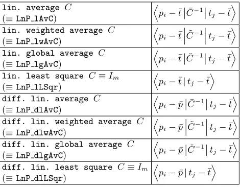
Table 3.Linear (differential) template attack variants.

lin. average C

(≡LnP lAvC)

D pi−¯_t

C¯−1 tj−¯t

E

lin. weighted average C

(≡LnP lwAvC)

D pi−¯t

˜

C−1 tj−¯t

E

lin. global average C

(≡LnP lgAvC)

D pi−¯_t

Cˇ−1 tj−¯t

E

lin. least square C≡Im

(≡LnP lLSqr)

D

pi−¯t|tj−¯tE

diff. lin. average C

(≡LnP dlAvC)

D

pi−p¯C¯

−1 tj−¯t

E

diff. lin. weighted average C

(≡LnP dlwAvC)

D pi−p¯

˜

C−1 tj−¯t

E

diff. lin. global average C

(≡LnP dlgAvC)

D

pi−p¯Cˇ

−1 tj−¯t

E

diff. lin. least square C≡Im

(≡LnP dlLSqr)

D

pi−p¯|tj−¯tE

averaging, two of which should converge in the limit of many traces taken. The standard average ¯C is simply given by

¯

C= 1

M

X

j

Cj , (4)

whereM is the number of templates, whilst ˜C is a weighted average, ˜

C= 1

M0

X

j

njCj , (5)

where as weights the number of traces nj pertinent to template j have been used, andM0=P

jnj. Clearly, these two definitions are identical whennj does not depend on j, or at least very nearly so, which is often the case for large data sets created with random data. However, when the target is not the value itself, but rather the Hamming weight, then this is not normally the case, as the Hamming weight distribution is highly uneven. Small and very large Hamming weights are much less frequently seen than average Hamming weights.

Yet another way to arrive at a normalised average covariance ˆC is to ex-pand on the idea underlying Eq. (3), and renormalise all covariancesCjprior to averaging such that all have the same determinant,

ˆ

C= 1

M

X

j

−mq_det(_C

j)Cj . (6)

(5)

But the most aggressive level of approximation is to assumeC≡Im, leading to

ln (Pij)≈ − D

pi−tj|pi−tj E

, (7)

which for obvious reasons is also referred to as the least–square approximation. If this variant is any good, then clearly it is the trivial mechanism of pattern matching, pj →tj for large nj, which is the dominant effect, and not a fancy structure ofC_j−1.

Finally, when we assumeCto be the same across all templates, anyway, then with a few more approximations it is possible to linearise all these expressions, where for instance Eq. (1) then becomes

ln (Pij)≈ D

pi−¯t C−1

tj−¯t

E

, (8)

where ¯t= (1/M0)P

jnjtj, andC being defined by either Eq. (4), or Eq. (5), or again by simply settingC≡Im. Please heed the opposite sign in this equation. On a finer point, it should be noted that the calculation of ¯tis done during the Profiling Phase, which in practice can introduce an unwanted offset into the differencepi−¯tneeded in the term multiplied toC−1 from the left in Eq. (8), with a negative impact on the accuracy of the resulting matching probability. It may thus be better to replace ¯t by the weighted average over all profiles, ¯

p= (1/N0₎P

in0ipi, obtained during the Exploitation Phase. This approximation tends to yield very poor results when the patterns are based on very few traces only. In such a situation the original linearisation is generally better, since the templates have been based on more traces, usually.

This trick of replacing ¯tby ¯pcan also be applied to all the non–linear variants of ln(P), by simply inserting the difference ¯p−¯_t_{on both sides of the bilinear form.} These variants of ln(P) may perform better when the traces in the Exploitation Phase have a systematic offset compared to those of the Profiling Phase.

All these approximations give a grand total of 24 different definitions for ln (Pij) — one original, one without the ln(det(Cj)) term, one with renormalised

Cj, four with different definitions of an averageC, one least–square variant, then eight variants of these first eight, where ¯p−_t¯_{got inserted on both sides, and} another eight different linearisations of some of the average variants of above. Tables 1, 2 and 3 provide an overview, including the naming convention used in all subsequent plots. The strength of these template attack variants may be vastly different and thus one should always inspect all of them, since the attacker can do so during the Profiling Phase and determine which one works best.

(6)

-50 0 50

EM Amplitude

100 80

60 40

20 0

x103

SingleTrace

Input Input

DES1 DES2

DES3

DES4

Output Output

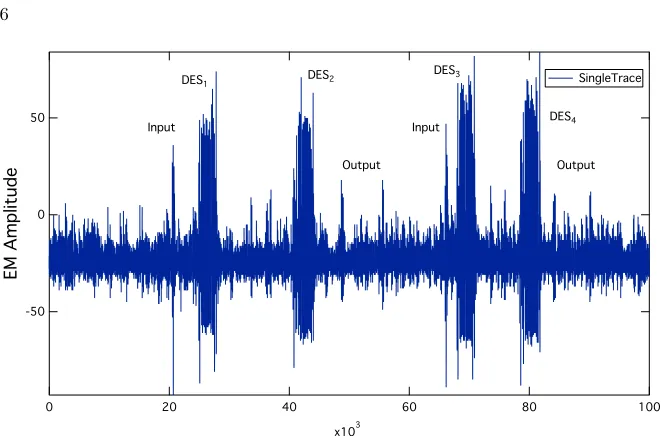
Fig. 1. A typical single EM trace of the TOE showing 4 calls to the DES hardware engine. It was obtained by placing a commercial Langer EM probe on top of what had previously been identified as a DES coprocessor hard macro in the chip layout. Sampling rate: 5 GS/s.

any two patternsiandi0 were to point to the same templatejas the most likely matching candidate. Consequently, a way needs to be found to eliminate pattern– template matchings that are not compatible with each other, and weeding out such inconsistencies should improve the ranking lists considerably. When all patterns relate to each other via a bijective xor mapping such that lnPi,i⊕j is the correct matching for patterni, then the joint probability distribution is given by the sum over all [13],

ln ˆPj = X

i

nilnPi,i⊕j , (9)

where the sum runs over all patternsi. When the template attack is successful,j

will point to the unknown common secretK. Another way of looking at Eq. (9) is to regard it as the product over all probabilities compatible with a particular valuej for the unknown common secret.

3 Results for a Contemporary Smart Card

(7)

-80 -60 -40 -20 0 20 40 60 80

EM Amplitude

12 10

8 6

4 2

0

x103

Average

DES1 DES2 DES3 DES4

Fig. 2.Average trace with all four DES blocks aligned.

10

8

6

4

2

Standard Deviation

12 10

8 6

4 2

0

x103

StdDev_Plain

DES1 DES2 DES3 DES4

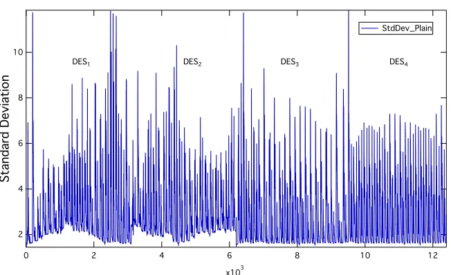
Fig. 3. Standard deviation with all four DES blocks aligned. The first DES block is the most difficult to align and far from perfect yet.

elastic alignment filter based on segment–wise parametrizing the internal clock / time asT =a+bt+ct2₊_dt3₊_et4₊_{f t}5_{, where}_t _{corresponds to the} exter-nal clock / time, and then finding the best set of coefficients (a, b, c, d, e, f) for each DES segment of each trace.1Starting with a little over 7M raw traces with

1

(8)

random plain text and random key, this procedure yielded just over 5M aligned traces, with their average trace given in Fig. 2, and its standard deviation shown in Fig. 3. Likely, the multiple calls to the DES hardware engine are due to coun-termeasures against fault attacks. We do not need to know whether these DES calls are “forward” or “backward” calculations — it does not matter, anyway, for launching a template attack, as long as they are static and do not change from one call to another. However, subsequent analysis reveals that these are forward – backward – forward – backward DES calls. Interestingly, they do not have precisely the same run–time behaviour, and also their standard deviations are slightly different as per Fig. 3. The last two DES blocks are much easier to align. Other than this alignment, no further preprocessing has been performed for calculating the templates later on.

The same procedure was then also applied to a further set of 2M raw traces, yielding 1.5M aligned traces in the end, where again the plain text was chosen randomly, but this time the key was kept fixed. This second set of traces will be used for the Exploitation Phase.

Fig. 4 shows strong leakage of the plain text, cipher text, as well as the key in the form of P[i]⊕P[i+ 4], C[i]⊕C[i+ 4], and K[i]⊕K[i+ 4], where

i = 0...3, and i refers to the i–th byte. This leakage is most likely due to the internal architecture of this DES hardware engine, where data are moved into the frontend of the coprocessor in portions of 32 bits, and then put into place inside the coprocessor in the next clock cycle. Without any blinding countermeasures this will lead to a Hamming distance leakage of the left half of the plain text with its right half, and similarly for cipher text and key. The timing of leakage seen in the trace indicates that except for the very first DES call, where the plain text does not seem to leak at all, plain text and key are handled in parallel, whilst the cipher text is naturally being handled at a later point in time. Because of this larger algorithmic noise, attacking the plain text and the key should be somewhat harder than attacking the cipher text. Naturally, at most half of the plain text, cipher text, and key bits are possible to recover with this attack.

In Figs. (5–6) we show the results of a template attack in Exploitation Phase using templates generated with 5M traces as input and 576 points of interest (POI), chosen based on aχ2 _analysis2 _{— and this for all 24 approximations to}

as a reference trace and then for each trace perform a least–square search for each of the 4 DES blocks separately to get a rough alignment of those 4 DES blocks. Secondly, the internal clock does not appear to be very stable. In the most simple approximation we assume the internal clock frequency to vary smoothly over time and model this with a polynomial fit. Since polynomial fits only work well over rather short time intervals, it then becomes necessary to split each DES block into a couple of time segments and apply the polynomial fit to each of them separately, using continuity equations as needed. Again, for each trace and each time segment, the best set of coefficients is determined using a least–square algorithm.

2 _{With canonical meanings of all variables, the definition of the}_χ2 _{function is given}

asχ2(t) = 1

n

1

mHW−1 PmHW

iHW=0niHW

(µi_HW(t)−µ(t))2

(9)

50

0

-50

Average

12 10

8 6

4 2

0

x103

0.20

0.15

0.10

0.05

0.00

-0.05

-0.10

-0.15

32-bit Correlation

C[i] ⊕ C[i+4]

P[i] ⊕ P[i+4] Average

-80 -60 -40 -20 0 20 40 60 80

Average

12 10

8 6

4 2

0

x103

0.15

0.10

0.05

0.00

-0.05

-0.10

32-bit Correlation

K[i] ⊕ K[i+4] Average

Fig. 4.Top: The 32–bit correlations ofP[i]⊕P[i+ 4] andC[i]⊕C[i+ 4],i= 0...3, show strong peaks up to≈20%. Bottom: The 32–bit correlation ofK[i]⊕K[i+ 4],i= 0...3, shows also strong peaks but to a large extent at the same positions and similar strength asP[i]⊕P[i+ 4].

Eq. (1) as discussed in Sec. 2. Plotted is the average ranking as a function of the number of traces ˜nused. Here the average is always taken over all possible 256 values of the patterns. To be more precise, e.g., ˜n = 1024 in Fig. 5, top part, means thatC[0]⊕C[4] is kept fixed for 1024 traces, whilst C[i]⊕C[i+ 4],

(10)

2 4 8 16 32 64 128

Ranking

1 2 4 8 16 32 64 128 256 512 1024 2048 4096

LnP

LnP_NormC LnP_NoDetC LnP_AvC LnP_wAvC LnP_gAvC LnP_nAvC

LnP_LSqr Exploitation C[0] ⊕ C[4]

LnP_lAvC LnP_lwAvC LnP_lgAvC LnP_lLSqr LnP_dlAvC LnP_dlwAvC LnP_dlgAvC LnP_dlLSqr

LnP_d LnP_dNormC LnP_dNoDetC LnP_dAvC LnP_dwAvC LnP_dgAvC LnP_dnAvC LnP_dLSqr

2 4 8 16 32 64 128

Ranking

1 2 4 8 16 32 64 128 256 512 1024 2048 4096

LnP

Fig. 5. Average rankings in Exploitation Phase for C[i]⊕C[i+ 4], i = 0...1, as a function of the number of traces used.

all 256 values ofC[0]⊕C[4]. In the end, an average is taken over all those 256 ranking results.

(11)

2 4 8 16 32 64 128

Ranking

1 2 4 8 16 32 64 128 256 512 1024 2048 4096

LnP

1 2 4 8 16 32 64 128

Ranking

1 2 4 8 16 32 64 128 256 512 1024 2048 4096

LnP

Fig. 6. Average rankings in Exploitation Phase for C[i]⊕C[i+ 4], i = 2...3, as a function of the number of traces used.

inversion, followed by a treatment for reducing the effect of constant offsets between Profiling and Exploitation Phase. Close runners up are LnP dNormC and LnP dNoDetC. In contrast, the original definition Eq. (1), i.e. LnP, is not effective at all.

(12)

4 8 16 32 64 128

Ranking

1 2 4 8 16 32 64 128 256 512 1024 2048 4096

LnP

LnP_NormC LnP_NoDetC LnP_AvC LnP_wAvC LnP_gAvC LnP_nAvC LnP_LSqr

Exploitation P[0] ⊕ P[4] LnP_lAvC

LnP_lwAvC LnP_lgAvC LnP_lLSqr LnP_dlAvC LnP_dlwAvC LnP_dlgAvC LnP_dlLSqr

4 8 16 32 64 128

Ranking

1 2 4 8 16 32 64 128 256 512 1024 2048 4096

LnP

LnP_LSqr Exploitation P[1] ⊕ P[5]

Fig. 7. Average rankings in Exploitation Phase for P[i]⊕P[i+ 4], i = 0...1, as a function of the number of traces used.

smaller) and, secondly, because the plain text leakage happens at the same time as the key leakage, which is a smart design choice.

(13)

8 16 32 64 128

Ranking

1 2 4 8 16 32 64 128 256 512 1024 2048 4096

LnP

8 16 32 64 128

Ranking

1 2 4 8 16 32 64 128 256 512 1024 2048 4096

LnP

Fig. 8. Average rankings in Exploitation Phase for P[i]⊕P[i+ 4], i = 2...3, as a function of the number of traces used.

text input of the second DES call is interrelated via a simple⊕, and thus Eq. (9) applies.

(14)

DES DES DES

DESi

DES

MAC

K1 K1 K1

K1 K2 P1

……

P2 Pk

IV

C1 C2

Fig. 9.ISO9797-1 MAC: IV, P1, P2 are all known and can be freely chosen. The attack according to [12] consists of a first step in which a side–channel attack in performed on the input of the second DES, which can be mapped back to the cipher text of the first DES, C1, and knowing IV and P1 a final brute–force attack is required to obtain the secret key K1 of the first DES.

Tables 4 and 5 show the results based on Eq. (9) and a chosen–plain–text attack. Here, ˜n = 256 means that each of the 256 possible pattern values has been selected precisely once for a given target byte, whilst ˜n= 1024 means each pattern value has been selected precisely four times.

For all four targetsP[i]⊕P[i+ 4],i= 0...3, the two approximations perform-ing consistently best areLnP lLSqrandLnP dlLSqr, which require between 256 and 2048 traces to achieve top rankings. It should be noted that although all the plain text bytes need to be chosen independently for each trace and each target byte anew, at least the choices for the first256 traces can be the same for all four target (⊕) bytes. Hence, those 256 traces can be reused and do not have to be counted four times when working out the total number of traces required to perform this attack.

(15)

10-7 10-6 10-5 10-4

28-bit

χ

2

12 10

8 6

4 2

0

x103

10-8 10-7 10-6 10-5 10-4 10-3

4 x 7-bit

χ

2

28-bit χ2 7-bit χ

2_{: K[0]}

⊕ K[4]

7-bit χ2: K[1] ⊕ K[5]

7-bit χ2: K[2] ⊕ K[6] 7-bit χ2: K[3] ⊕ K[7]

Fig. 10.χ2 _{leakage for} _K_[_i_]_⊕_K_[_i_{+ 4],} _i_{= 0}_..._{3, individually, as well as aggregated} over all 28 bits.

Next, we investigate the leakage of the key more closely. In Fig. 10 we have plotted theχ2_{leakage for each 7-bit target}_K_[_i_]_⊕_K_[_i_+4],_i_{= 0}_..._{3, separately, as} well as theχ2 _{leakage aggregated over all 28 bits. Four regions leak particularly,} but there are some smaller peaks also seen inbetween, where, e.g., K[0]⊕K[4] leaks, but none of the other three does.

Figs. 11 and 12 show the rankings obtained for K[i]⊕K[i+ 4], i = 0...3, for a fixed but randomly chosen key, using 1696 POI that had been derived from a χ2 analysis of Fig. 10. The fact that the key is fixed and only the plain text is randomly chosen does have a detrimental effect on the strength of the attack. Only some of the 24 approximations to Eq. (1) seem to converge to better ranking values, but none achieves top rank 1. For instance, LnP dstays fairly constant at rankings 5, 15, 36, and 16, respectively. On the other hand, the approximations LnP lAvC, LnP lwAvC, andLnP lgAvC start out somewhat poorly, but then converge to values≈11...32. This means a little over 2 bits leak per 7 bits, or some 8 – 10 bits of the 56–bit key, and this for as little as a few hundred traces (or even a single trace3_{in the case of}_{LnP d}_).

Presumably, this lack of convergence has to do with the fact that the tem-plates chosen are smaller than the number of fixed bits (i.e., bits that are kept constant for all traces) that leak at the same time, and thus can “interfere” with each other (cross–talk). For instance, whilst according to Fig. 4 the leakage correlation amplitudes for plain text, cipher text as well as key are all of simi-lar amplitude, the plain and cipher text turn out to be much more vulnerable

(16)

2 4 8 16 32 64

Ranking

20 22 24 26 28 210 212 214 216 218 220

LnP LnP_NormC LnP_NoDetC LnP_AvC LnP_wAvC LnP_gAvC LnP_nAvC LnP_LSqr

Exploitation K[0] ⊕ K[4] LnP_lAvC

LnP_lwAvC LnP_lgAvC LnP_lLSqr LnP_dlAvC LnP_dlwAvC LnP_dlgAvC LnP_dlLSqr LnP_d

LnP_dNormC LnP_dNoDetC LnP_dAvC LnP_dwAvC LnP_dgAvC LnP_dnAvC LnP_dLSqr

2 4 8 16 32 64

Ranking

20 22 24 26 28 210 212 214 216 218 220

Exploitation K[1] ⊕ K[5]

Fig. 11. Average rankings in Exploitation Phase for K[i]⊕K[i+ 4], i = 0...1, as a function of the number of traces used.

(17)

For instance, one could attack the Hamming weight of the entire 28–bit vector4_, or use larger template sizes, e.g., 14 bits per template. In any case, since the key is attacked directly, these results are straight–forwardly applicable to TDES without the need to invoke meet–in–the–middle attacks and the like.

4 8 16 32 64 128

Ranking

20 22 24 26 28 210 212 214 216 218 220

4 8 16 32 64

Ranking

20 22 24 26 28 210 212 214 216 218 220

Fig. 12. Average rankings in Exploitation Phase for K[i]⊕K[i+ 4], i = 2...3, as a function of the number of traces used.

(18)

It is, of course, possible to combine this leakage of the key with the leakage of the plain and cipher text to create an even stronger attack on ISO9797-1 MAC, since it would help to reduce the remaining brute–force attack on the key by performing the brute–force attack on the ranked lists.

4 Conclusions

In conclusion we have shown that it is worth spending some effort on analysing a variety of approximations to the standard probability density function of the multivariate normal distribution, Eq. (1), when applying this to template at-tacks. Some approximations yield substantially and consistently so better results than others. Generally, approximations based on averaged covariance matrices seem to perform consistently better, and measures to reduce the effects of con-stant offsets between templates and patterns are also beneficial. In any case, the attacker can always study during the Profiling Phase which approximation is likely to yield the best results in the Exploitation Phase.

As an example, we have studied the attack on the ISO9797-1 MAC, applied to a fairly recent smart card, which exhibits leakage of plain text, cipher text, as well as the secret key itself during a DES calculation. Only some 4K traces are required to perform the attack, and this does not yet include the possibility of making trade-offs between the number of measurement traces taken on the one hand, and the remaining brute–force effort required on the other hand.

The analysis of the key leakage requires more work. Preliminary results in-dicate leakage of about 6 – 10 bits per DES, and thus 18 – 30 bits per TDES.

For this particular platform the issue becomes even more severe as it is using a DES hardware coprocessor built in what is called a hard–macro design tech-nology, meaning that it is a design block with fixed geometry all the way down to the gate level. This hard macro is thus visible in the layout, and it is used in many other products in precisely the same shape over and over again. Hence, once a weakness such as this one has been found in one family member, it can be found in all other family members as well. Worse still, one has to assume that templates generated for one family member will be applicable for all other family members as well.

References

1. Kocher, P.C., Jaffe, J., Jun, B.: Differential power analysis. In: Wiener, M.J. (ed.) Advances in Cryptology - CRYPTO ’99, 19th Annual International Cryp-tology Conference, Santa Barbara, California, USA, August 15-19, 1999, Proceed-ings. Lecture Notes in Computer Science, vol. 1666, pp. 388–397. Springer (1999), http://dx.doi.org/10.1007/3-540-48405-1 25

(19)

3. Gierlichs, B., Batina, L., Preneel, B., Verbauwhede, I.: Revisiting higher-order DPA attacks:. In: Pieprzyk, J. (ed.) Topics in Cryptology - CT-RSA 2010, The Cryptographers’ Track at the RSA Conference 2010, San Francisco, CA, USA, March 1-5, 2010. Proceedings. Lecture Notes in Computer Science, vol. 5985, pp. 221–234. Springer (2010), http://dx.doi.org/10.1007/978-3-642-11925-5 16 4. Xiao, L., Heys, H.M.: A simple power analysis attack against the key

sched-ule of the camellia block cipher. Inf. Process. Lett. 95(3), 409–412 (2005), http://dx.doi.org/10.1016/j.ipl.2005.03.013

5. Chari, S., Rao, J.R., Rohatgi, P.: Template attacks. In: Jr., B.S.K., Ko¸c, C¸ .K., Paar, C. (eds.) Cryptographic Hardware and Embedded Systems - CHES 2002, 4th International Workshop, Redwood Shores, CA, USA, August 13-15, 2002, Revised Papers. Lecture Notes in Computer Science, vol. 2523, pp. 13–28. Springer (2002), http://dx.doi.org/10.1007/3-540-36400-5 3

6. Archambeau, C., Peeters, E., Standaert, F., Quisquater, J.: Template attacks in principal subspaces. In: Goubin, L., Matsui, M. (eds.) Cryptographic Hardware and Embedded Systems - CHES 2006, 8th International Workshop, Yokohama, Japan, October 10-13, 2006, Proceedings. Lecture Notes in Computer Science, vol. 4249, pp. 1–14. Springer (2006), http://dx.doi.org/10.1007/11894063 1

7. Medwed, M., Oswald, E.: Template attacks on ECDSA. In: Chung, K., Sohn, K., Yung, M. (eds.) Information Security Applications, 9th International Work-shop, WISA 2008, Jeju Island, Korea, September 23-25, 2008, Revised Selected Papers. Lecture Notes in Computer Science, vol. 5379, pp. 14–27. Springer (2008), http://dx.doi.org/10.1007/978-3-642-00306-6 2

8. Fouque, P., Leurent, G., R´eal, D., Valette, F.: Practical electromagnetic template attack on HMAC. In: Clavier, C., Gaj, K. (eds.) Cryptographic Hardware and Em-bedded Systems - CHES 2009, 11th International Workshop, Lausanne, Switzer-land, September 6-9, 2009, Proceedings. Lecture Notes in Computer Science, vol. 5747, pp. 66–80. Springer (2009), http://dx.doi.org/10.1007/978-3-642-04138-9 6 9. Choudary, O., Kuhn, M. G., Efficient Template Attacks in Smart Card Research

and Advanced Applications. Springer International Publishing, 2013:253-270 10. Hu, Y.B., Zhang, C., Zheng, Y.Y., Wagner, M.: Ciphertext and Plaintext Leakage

Reveals the Entire TDES Key. Cryptology ePrint Archive, Report 2016/1143, 2016 11. http://en.wikipedia.org/wiki/Bra-ket notation

12. Feix, B., Thiebeauld, H.: Defeating ISO9797-1 MAC algo 3 by combining side-channel and brute force techniques. Cryptology ePrint Archive, Report 2014/702, 2014

(20)

Table 4.Rankings forP[0]⊕P[4] andP[1]⊕P[5] based on Eq. (9).

˜

n LnP LnP NormC LnP NoDetC LnP AvC LnP wAvC LnP gAvC LnP nAvC LnP LSqr

256 101 108 101 1 1 1 1 5

512 3 3 3 1 1 1 1 1

1024 1 1 1 1 1 1 1 1

2048 1 1 1 1 1 1 1 1

4096 2 2 2 1 1 1 1 1

8192 1 1 1 1 1 1 1 1

16384 1 1 1 1 1 1 1 1

˜

n LnP d LnP dNormC LnP dNoDetC LnP dAvC LnP dwAvC LnP dgAvC LnP dnAvC LnP dLSqr

256 100 106 100 1 1 1 1 5

512 3 3 3 1 1 1 1 1

1024 1 1 1 1 1 1 1 1

2048 1 1 1 1 1 1 1 1

4096 2 2 2 1 1 1 1 1

8192 1 1 1 1 1 1 1 1

16384 1 1 1 1 1 1 1 1

˜

n LnP lAvC LnP lwAvC LnP lgAvC LnP lLSqr LnP dlAvC LnP dlwAvC LnP dlgAvC LnP dlLSqr

256 1 1 1 5 1 1 1 5

512 1 1 1 1 1 1 1 1

1024 1 1 1 1 1 1 1 1

2048 1 1 1 1 1 1 1 1

4096 1 1 1 1 1 1 1 1

˜

256 196 188 196 3 3 3 3 7

512 79 76 79 1 1 1 1 5

1024 23 22 23 1 1 1 1 1

2048 17 17 17 1 1 1 1 1

4096 1 1 1 1 1 1 1 1

8192 1 1 1 1 1 1 1 1

16384 1 1 1 1 1 1 1 1

˜

256 195 182 195 3 3 3 3 7

512 67 62 67 1 1 1 1 5

1024 21 20 21 1 1 1 1 1

2048 15 15 15 1 1 1 1 1

4096 1 1 1 1 1 1 1 1

8192 1 1 1 1 1 1 1 1

16384 1 1 1 1 1 1 1 1

˜

256 3 3 3 7 3 3 3 7

512 1 1 1 5 1 1 1 5

1024 1 1 1 1 1 1 1 1

2048 1 1 1 1 1 1 1 1

(21)

Table 5.Rankings forP[2]⊕P[6] andP[3]⊕P[7] based on Eq. (9).

˜

256 34 36 34 2 2 2 2 51

512 12 10 12 1 1 1 1 4

1024 4 4 4 1 1 1 1 2

2048 1 1 1 1 1 1 1 1

4096 72 73 72 1 1 1 1 1

8192 6 6 6 1 1 1 1 1

16384 1 1 1 1 1 1 1 1

˜

256 38 37 38 2 2 2 2 51

512 10 10 10 1 1 1 1 4

1024 4 4 4 1 1 1 1 2

2048 1 1 1 1 1 1 1 1

4096 63 63 63 1 1 1 1 1

8192 3 3 3 1 1 1 1 1

16384 1 1 1 1 1 1 1 1

˜

256 2 2 2 51 2 2 2 51

512 1 1 1 4 1 1 1 4

1024 1 1 1 2 1 1 1 2

2048 1 1 1 1 1 1 1 1

4096 1 1 1 1 1 1 1 1

˜

256 129 121 129 5 5 5 5 1

512 21 15 21 1 1 1 1 1

1024 1 1 1 3 3 3 3 1

2048 2 2 2 2 2 2 2 1

4096 1 1 1 1 1 1 1 1

8192 4 4 4 1 1 1 1 1

16384 1 1 1 1 1 1 1 1

˜

256 134 130 134 5 5 5 5 1

512 29 26 29 1 1 1 1 1

1024 1 1 1 3 3 3 3 1

2048 2 2 2 2 2 2 2 1

4096 1 1 1 1 1 1 1 1

8192 3 3 3 1 1 1 1 1

16384 1 1 1 1 1 1 1 1

˜

256 5 5 5 1 5 5 5 1

512 1 1 1 1 1 1 1 1

1024 3 3 3 1 3 3 3 1

2048 2 2 2 1 2 2 2 1