Implementing Pairings at the 192-bit Security
Level
Diego F. Aranha1, Laura Fuentes-Casta˜neda2, Edward Knapp3, Alfred Menezes3, and Francisco Rodr´ıguez-Henr´ıquez2
1 Department of Computer Science, University of Bras´ılia
2 CINVESTAV-IPN, Computer Science Department
[email protected], [email protected]
3 Department of Combinatorics & Optimization, University of Waterloo
[email protected], [email protected]
Abstract. We implement asymmetric pairings derived from Kachisa-Schaefer-Scott (KSS), Barreto-Naehrig (BN), and Barreto-Lynn-Scott (BLS) elliptic curves at the 192-bit security level. Somewhat surprisingly, we find pairings derived from BLS curves with embedding degree 12 to be the fastest for our serial as well as our parallel implementations. Our serial implementations provide a factor-3 speedup over the previous state-of-the-art, demonstrating that pairing computation at the 192-bit security level is not as expensive as previously thought. We also present a general framework for deriving a Weil-type pairing that is well-suited for computing a single pairing on a multi-processor machine.
1
Introduction
Since the advent of pairing-based cryptography, researchers have been devising methods for constructing and efficiently implementing bilinear pairings. Initial work [5,12] was focused on implementing pairings at (roughly) the 80-bit se-curity level. Koblitz and Menezes [19] highlighted the performance drawbacks of pairings at very high security levels. The subsequent discovery of Barreto-Naehrig (BN) elliptic curves [7], ideally suited for implementing pairings at the 128-bit security level, spurred a lot of research culminating in the implemen-tation of Aranha et al. [2] that achieved speeds of under 2 million cycles for a 128-bit pairing computation on a single core of Phenom II, Core i5 and Opteron machines.
choice of pairing to implement a particular protocol can depend on a variety of factors including the number and complexity of non-pairing operations in the protocol, the number of pairing computations that are required, and the appli-cability of several optimizations including fixed-argument pairings and products of pairings [27].
In this paper, we focus on fast implementations of a single pairing at the 192-bit security level. We chose the 192-bit level because it is the higher security level (the other is 128-bit) for public-key operations in the National Security Agency’s Suite B Cryptography standard [23]. Moreover, as mentioned by Scott [28], the optimum choice of pairing-friendly curve for the 192-bit security level from the many available candidates [10] is not straightforward.
We examine a family of embedding degreek= 12 elliptic curves, henceforth calledBLS12 curves, first proposed by Barreto, Lynn and Scott [6] (see also [8]). Unlike BN curves, the BLS12 curves are not ideal for the 128-bit security level since the group order #E(Fp) is not prime. Nevertheless, our careful estimates
and implementation results demonstrate that they outperform KSS, BN and BLS24 curves at the 192-bit security level. We also present a general framework for deriving analogues of theβ Weil pairing, first presented in [3] for BN curves. This pairing is well-suited for computing a single pairing on a multi-processor machine since it avoids the relatively-costly final exponentiation that cannot be effectively parallelized and is present in all Tate-type pairings.
The remainder of the paper is organized as follows. The salient parameters of KSS, BN, BLS12 and BLS24 curves are presented in§2. In§3, we review Ver-cauteren’s notion of an optimal pairing and present theβWeil pairing. The cost of the BLS12, KSS, BN and BLS24 pairings are estimated in§4,§5,§6 and§7, respectively. Finally,§8 compares the estimated speeds of the four pairings and reports on our implementation. Our results show a significant performance im-provement over the previous state-of-the-art for serial pairing implementation of the optimal ate pairing at the 192-bit security level, and an increased scalability of theβ Weil pairing in relation to the optimal ate pairing.
2
Pairing-friendly elliptic curves
Letpbe a prime, and letEbe an elliptic curve defined over the finite fieldFp. Let
rbe a prime withr|#E(Fp) and gcd(r, p) = 1. Thecofactor isρ= logp/logr.
Theembedding degree kis the smallest positive integer withr|(pk−1). We will
assume thatkis even, whencek >1 andE[r]⊆E(Fpk).
Letπ : (x, y) 7→ (xp, yp) be the p-th power Frobenius endomorphism. The
trace of the Frobenius is t =p+ 1−#E(Fp). Let G1 = {P ∈ E[r] : π(P) = P}=E(Fp)[r];G1is the 1-eigenspace ofπacting onE[r]. Letdbe the order of the automorphism group of E, and suppose that d|k. Lete=k/dandq=pe.
Then there is a unique degree-dtwist ˜E of E overFq with r|# ˜E(Fq) [16]; let
Ψ : ˜E →E be the associated twisting isomorphism. Let ˜Q∈E(˜ Fq) be a point
study in this paper are non-degenerate bilinear maps fromG1×G2 to GT and
are called Type 3 pairings in the literature [13].
Table 1 summarizes the salient parameters of the KSS [17], BN [7], BLS12 [6] and BLS24 [6] families of elliptic curves. All these curves are parameterized by a positive integerz, are defined by an equation of the formY2=X3+b, and have a twist of order d= 6. Table 2 lists the important parameters of the particular KSS, BN, BLS12 and BLS24 curves that are suitable for implementing pairing-based protocols at the 192-bit security level. The requirements for this security level are that the bitlength of rbe at least 384 (in order to resist Pollard’s rho attack [25] on the discrete logarithm problem inG1), and that the bitlength of pk should be at least 7680 (in order to resist the number field sieve attack [26]
on the discrete logarithm problem inF∗pk).
KSS curves: k= 18, ρ≈4/3
p(z) = (z8+ 5z7+ 7z6+ 37z5+ 188z4+ 259z3+ 343z2+ 1763z+ 2401)/21 r(z) = (z6+ 37z3+ 343)/343, t(z) = (z4+ 16z+ 7)/7
BN curves: k= 12, ρ≈1 p(z) = 36z4+ 36z3+ 24z2+ 6z+ 1
r(z) = 36z4+ 36z3+ 18z2+ 6z+ 1, t(z) = 6z2+ 1
BLS12 curves: k= 12, ρ≈1.5
p(z) = (z−1)2(z4−z2+ 1)/3 +z, r(z) =z4−z2+ 1, t(z) =z+ 1
BLS24 curves: k= 24, ρ≈1.25
p(z) = (z−1)2(z8−z4+ 1)/3 +z, r(z) =z8−z4+ 1, t(z) =z+ 1
Table 1. Important parameters for the KSS, BN, BLS12 and BLS24 families.
Curve b k z ⌈log2p⌉ ⌈log2r⌉ ρ ⌈log2q⌉ ⌈log2p k⌉ KSS 2 18 −264−251+ 246+ 212 508 376 1.35 1523 9137
BN 5 12 2158−2128−268+ 1 638 638 1 1275 7647 BLS12 4 12 −2107+ 2105+ 293+ 25 638 427 1.49 1276 7656 BLS24 4 24 −248+ 245+ 231−27 477 383 1.25 1914 11482
Table 2.Important parameters for the chosen KSS, BN, BLS12, BLS24 curves.
3
Optimal pairings
LetR∈E(Fpk) and letsbe a non-negative integer. AMiller function fs,R [22]
oflengthsis a function inFpk(E) with divisor (fs,R) =s(R)−(sR)−(s−1)(∞).
functions are minimally defined; that is, ifR∈E(Fpℓ), thenfs,Ris selected from
the function fieldFpℓ(E).
The optimal ate pairing.Vercauteren’s optimal pairing framework [30] allows one to compute a pairing using Miller functions each of length approximately (1/φ(k)) logr.
For a pointR∈E[r] and polynomialh=∑hixi∈Z[x] such thath(s)≡0
(mod r), define theextended Miller functionfs,h,Rto be the normalized rational
function with divisor
deg∑h
i=0
hi[(siR)−(∞)].
Thelengthof the extended Miller functionfs,h,Ris the maximum of the absolute
values of the hi’s. Observing thatfs,h1,R·fs,h2,R=fs,h1+h2,Rand the
polyno-mials h(x) =r,h(x) =xi−pi satisfy the congruence condition withs=p, we desire elements in the following lattice which have small coefficients:
[
r(z) 0 v Iφ(k)−1
]
,
wherevis the column vector withi-th entry−p(z)i. This leads to the following
result of Vercauteren’s.
Theorem 1 ([30]). There exists h such that |hi| ≤ r1/φ(k) and (P, Q) 7→
fp,h,Q(P)(p
k−1)/r
is a pairing.
For parameterized curves, the function fp,h,Q where |hi| ≤ r1/φ(k) can be
computed as a product of Miller functions each having length approximately (1/φ(k)) logr. Optimal ate pairings for KSS [30], BN [30], BLS12 [16] and BLS24 [16] curves are given in Table 3. In the table,ℓS,T denotes the line through points
S andT.
Curve Optimal ate pairing: (P, Q)7→ h(x)
KSS (fz,Q·f3p,Q·ℓz[Q],[3p]Q(P)
)(p18−1)/r
z+ 3x−x4
BN (f6z+2,Q·ℓ[6z+2]Q,[p]Q·ℓ[6z+2+p]Q,[−p2]Q(P)
)(p12−1)/r
6z+ 2 +x−x2+x3
BLS12 (fz,Q(P))(p12−1)/r z−x BLS24 (fz,Q(P))(p24−1)/r z−x
Table 3.Optimal ate pairings.
The β Weil pairing. Set k =ed, where d is the order of the automorphism group of E. Define wsandws,h as
ws(P, Q) = (
fs,Q(P)
fs,P(Q)
)pk/2−1
and ws,h(P, Q) = (
fs,h,Q(P)
fs,h,P(Q)
)pk/2−1
Hess [15] gave a framework for computing optimal Weil pairings, building on the methods of Vercauteren as expressed in Theorem 1.
Theorem 2 (Theorem 1 in [15]). There exists h such that |hi| ≤ r1/2 and
wpe,his a pairing.
The pairing wpe,h with |hi| ≤ r1/2 can be computed using two extended Miller functions of length approximately 12logr. We present a framework for constructing Weil-type pairings, called β pairings, which can be computed us-ing 2eextended Miller functions each of length approximately (1/φ(k)) logr. In particular, we prove that for a polynomial h for whichh(p) ≡0 (modr), the following is a pairing:
β:G1×G2→GT : (P, Q)7→ e∏−1
i=0
wp,h([pi]P, Q)p
e−1−i
. (2)
To establish that (2) is a pairing, we require a few technical lemmas, building on the work of Hess and Vercauteren. Lemma 1 gives a pairing which is the product of Weil pairings consisting of Miller functions having ate-like lengths.
Lemma 1. For all positive integerss, the following map from G1×G2 to GT
is a pairing:
(P, Q)7→
(e−1 ∏
i=0
(
fps,[pi]Q(P) fps,[pi]P(Q)
)pe−1−i)p
k/2−1
.
Proof. It follows from Theorem 1 of [15] that the map
(P, Q)7→
(
fpe,Q(P) fpe,P(Q)
)pk/2−1
is a pairing. Using Lemma 3(ii), one can see that
fpe,P =
e∏−1
i=0
(fp,[pi]P)p e−1−i
.
Hence, the result holds fors= 1. Since
fps,P =
s∏−1
j=0
(fp,[pj]P)p s−1−j
we have that
e∏−1
i=0
(fps,[pi]P)p e−1−i
=
e∏−1
i=0
s∏−1
j=0
(fp,[pi][pj]P)p s−1−j
pe−1−i
=
s∏−1
j=0
(e−1 ∏
i=0
(fp,[pi]([pj]P))p e−1−i
)ps−1−j
=
s∏−1
j=0
(
fpe,[pj]P
)ps−1−j .
From this, we can observe that
(e−1 ∏
i=0
(
fps,[pi]Q(P) fps,[pi]P(Q)
)pe−1−i)pk/2−1 =
(s−1 ∏
i=0
(
fpe,[pi]Q(P) fpe,[pi]P(Q)
)ps−1−i)pk/2−1 . (3)
By Lemma 6 of [14], the map (P, Q)7→ fpe,Q(P) is a pairing. Thus, the right hand side of (3) is a product of pairings. □
The next lemma relates the previous pairing to the Weil pairing notation defined in (1).
Lemma 2. The following identity holds for all positive integerss:
(e−1 ∏
i=0
(
fps,[pi]Q(P) fps,[pi]P(Q)
)pe−1−i)pk/2−1 =
e−1
∏
i=0
wps([pi]P, Q)p e−1−i
.
Proof. By Lemma 6 of [14], the map (P, Q)7→fps,Q(P) is a pairing and so
(e−1 ∏
i=0
(
fps,[pi]Q(P)
fps,[pi]P(Q)
)pe−1−i)pk/2−1 =
(e−1 ∏
i=0
(
fps,Q([pi]P) fps,[pi]P(Q)
)pe−1−i)pk/2−1
=
e∏−1
i=0
wps([pi]P, Q)p e−1−i
. □
Finally, using the pairing relation from Lemma 2, we can obtain a pairing composed of Miller functions each with Vercauteren-style bound on the length.
Theorem 3. There exists h such that |hi| ≤ r1/φ(k) and the following is a
pairing:
β:G1×G2→GT : (P, Q)7→ e∏−1
i=0
wp,h([pi]P, Q)p
Proof. Leth(x) =∑ci=0hixi be given by Vercauteren’s theorem and leth(p) =
rm. Since
fr,Pm =fp,h,P· c ∏
j=0 fhj
pj,P,
we have that
wr(P, Q)m=wp,h(P, Q)· c ∏
j=0
wpj(P, Q)hj.
Hence
e∏−1
i=0
wp,h([pi]P, Q)p
e−1−i =
e∏−1
i=0
wr([pi]P, Q)m· c ∏
j=0
wpj([pi]P, Q)−hj
pe−1−i
=
e∏−1
i=0
wr([pi]P, Q)mp
e−1−i
· c ∏
j=0
(e−1 ∏
i=0
wpj([pi]P, Q)p e−1−i
)−hj ,
which by Lemmas 1 and 2 is a product of pairings. □
Using Theorem 3 and the polynomialshfrom Table 3, we found that the β Weil pairings for BN, BLS12, KSS and BLS24 curves can be defined as follows:
KSS : (P, Q)7→
[(
fp,h,P(Q)
fp,h,Q(P) )p2(
fp,h,[p]P(Q)
fp,h,Q([p]P) )p
fp,h,[p2]P(Q)
fp,h,Q([p2]P)
](p9−1)(p3+1) ,
(4)
BN : (P, Q)7→
[(
fp,h,P(Q)
fp,h,Q(P) )p
fp,h,[p]P(Q)
fp,h,Q([p]P)
](p6−1)(p2+1)
, (5)
BLS12 : (P, Q)7→
[(
fz,P(Q)
fz,Q(P) )p f
z,[p]P(Q)
fz,Q([p]P)
](p6−1)(p2+1)
, (6)
BLS24 : (P, Q)7→
f
p3 z,P(Q)·f
p2
z,[p]P(Q)·f p
z,[p2]P(Q)·fz,[p3]P(Q)
fz,Qp3 (P)·fz,Qp2 ([p]P)·fz,Qp ([p2]P)·f
z,Q([p3]P)
(p12−1)(p4+1)
.
(7) For all fourβ Weil pairings, computing [p]P has approximately the same cost as computing [z]P.
Lemma 3. Let a and b be non-negative integers, and let R ∈ E(Fqk). Then (i) fa+b,R = fa,R·fb,R ·ℓ[a]R,[b]R/v[a+b]R, where vP denotes the vertical line
through P; and (ii) fab,R =fb,Ra ·fa,[b]R.
The method of Aranha et al. [4] for parallelizing the computation of a Miller functionfs,Ris the following. We first writes= 2ws1+s0withs0<2w. Applying Lemma 3, we obtain
fs,R =f2
w
s1,R·f2w,[s1]R·fs0,R·ℓ[2ws1]R,[s0]R/v[s]R. (8)
Ifs0is small, then the Miller functionfs0,Rcan be computed relatively cheaply.
Thus the computation of fs,R can be parallelized by computing f2
w
s1,R on one
processor andf2w,[s
1]Ron a second processor. The parameterwshould be
care-fully selected in order to balance the time of the two function computations. The relevant criteria for selecting w include the Hamming weight ofs1 (which determines the number of additions in the Miller loop for the first function), and the cost of thew-fold squaring in the first function relative to the cost of computings1Rin the second function. This idea can be extended tocprocessors by writings= 2wc−1s
c−1+· · ·+ 2w1s1+s0.
Remark 1. (unsuitability of composite-order BN curves) Consider a BN curve at the 192-bit security level. For such a curve, we desire a (sparse) BN parameter z of approximately 160 bits. From the optimal pairing framework, we choose a suitable vector [2z, z+ 1,−z, z] corresponding to the following pairing (with the final exponentiation omitted):
(P, Q)7→f2z,Q·fzp+1,Q·f−p 2 z,Q ·f
p3
z,Q·ℓ[−zp2]Q,[zp3]Q·ℓ[p(z+1)]Q,[−zp2+zp3]Q(P).
Computation of the lines is relatively inexpensive. However, at first, it ap-pears one must evaluate multiple Miller functions. Fortunately, for parameterized curves, one can (usually) rearrange terms such that the computational bottle-neck isfz,Qwith only a few lines comprising the remaining computation. In the
above case, we obtain
(P, Q)7→fz,Q2+p−p2+p3·ℓ[z]Q,[z]Q·ℓ[zp]Q,[p]Q·ℓ[−zp2]Q,[zp3]Q·ℓ[p(z+1)]Q,[−zp2+zp3]Q(P).
At the 192-bit security level, we require thatrhave a prime divisor of at least 384 bits. We can easily chooserto be (a 640-bit) prime. However, given that the optimal pairing framework gives a maximum Miller length of around (logn)/4 for BN curves where n is a large prime divisor of r, we should be tempted to chooserwith a 384-bit prime divisor. The fact that the coordinates of the vector [2z, z+1,−z, z] have small coefficients when written in basezallowed us to write the pairings as a power offz,Qmultiplied by a few lines. However, for composite
than the Tate pairing. The possibility of choosing a vector whose elements are part of a short addition chain may still exist but the vectors produced by the LLL algorithm [21] do not appear to maintain such structure. Thus, composite-order BN curves would appear to yield inferior performance compared to prime-order BN curves.
4
BLS12 pairings
In this section, we consider the BLS12 curve Y2 = X3+ 4 defined with the parameter selection z=−2107+ 2105+ 293+ 25 which yields a 638-bit primep and a 427-bit primer.
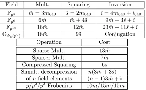
Extension field arithmetic for pairings with k=12. A tower extension forFp12 can be constructed as follows:
Fp2 =Fp[u]/(u2−β), whereβ ∈Fp, Fp6 =Fp2[v]/(v3−ξ), whereξ∈Fp2, and Fp12 =Fp6[w]/(w2−γ), whereγ∈Fp6.
For our choice of parameters, we have the optimal β =−1,ξ =u+ 1, γ =v. Table 4 gives the computational costs of the tower extension field arithmetic for curves with k = 12 in terms of a 640-bit multiplication (m640) and inversion (i640) inFp, withpa 638-bit prime.1The cost of additions is ignored because of
their lower overall performance impact due to the larger field size in comparison with [2,24]. Moreover, ˜m, ˜s, ˜ıdenote the cost of multiplication, squaring and inversion inFp2 respectively.2GΦ
6(p2)denotes the order-Φ6(p
2) subgroup ofF∗
p12,
whereΦk denotes thek-th cyclotomic polynomial.
Miller loop. For the parameter selection z = −2107+ 2105+ 293+ 25, the Miller loop computation offz,Q requires 107 point doublings and associated line
evaluations, 3 point additions with line evaluations, 109 sparse multiplications, and 106 squarings in Fp12. The computational costs of these operations can
be found in [2, Table 1]. We obtain a BLS12 Miller loop cost of 107(3 ˜m+ 6˜s+ 4m640)+3(11 ˜m+2˜s+4m640)+109(13 ˜m)+106(12 ˜m) = 3043 ˜m+648˜s+440m640= 10865m640.
Final exponentiation.The final exponentiation consists of raising the Miller loop resultf ∈Fpk to thee= (pk−1)/r-th power. This task can be broken into two parts since
e= (pk−1)/r= [(pk−1)/Φk(p)]·[Φk(p)/r].
Computing f(pk−1)/Φk(p) is considered easy, costing only a few multiplications, inversions, and inexpensive p-th powerings in Fpk. Raising to the power d = 1 In the case of software implementation, this selection of the size ofpfacilitates the
usage oflazy reductiontechniques as recommended in [2,24]. 2
Field Mult. Squaring Inversion
Fp2 m˜ = 3m640 s˜= 2m640 ˜ı= 4m640+i640
Fp6 6 ˜m m˜ + 4˜s 9 ˜m+ 3˜s+ ˜ı
Fp12 18 ˜m 12 ˜m 23 ˜m+ 11˜s+ ˜ı GΦ6(p2) 18 ˜m 9˜s Conjugation
Operation Cost
Sparse Mult. 13 ˜m Sparser Mult. 7 ˜m Compressed Squaring 6˜s Simult. decompression n(3 ˜m+ 3˜s)+
ofnfield elements (n−1)3 ˜m+ ˜ı p/p2/p3-Frobenius 10m/15m/15m
Table 4. Costs of arithmetic operations in a tower extension fieldFp12.
Φk(p)/r is a more challenging task. Observing that p-th powering is much less
expensive than multiplication, Scott et al. [29] give a systematic method for reducing the expense of exponentiating byd. In the case of BLS12 curves, it can be shown that the exponent d can be written as d= λ0+λ1p+λ2p2+λ3p3 whereλ0=z5−2z4+ 2z2−z+ 3,λ1=z4−2z3+ 2z−1,λ2=z3−2z2+z, and λ3 =z2−2z+ 1. The exponentiation fd can be computed using the following addition-subtraction chain:
f →f−2→fz→f2z→fz−2→fz2−2z→fz3−2z2 →fz4−2z3
→fz4−2z3+2z→fz5−2z4+2z2,
which requires 5 exponentiations byz, 2 multiplications inFp12, and 2 cyclotomic
squarings. This allowsfd to be computed as
fd=fz5−2z4+2z2·(fz−2)−1·f·(fz4−2z3+2z·f−1)p·(fz3−2z2·fz)p2·(fz2−2z·f)p3,
which requires an additional 8 multiplications in Fp12 and 3 Frobenius maps.
This implies that the hard part of the final exponentiation requires 2 cyclotomic squarings, 5 exponentiations by z, 10 multiplications in Fp12, and 3 Frobenius
maps.
In total, the cost of computing the final exponentiation is 1 inversion in
Fp12, 2 cyclotomic squarings, 12 multiplications in Fp12, 4 Frobenius maps, and
5 exponentiations byz. It can be shown that exponentiation by our choice of the z parameter requires 107 compressed squarings, simultaneous decompression of 4 field elements, and 3 multiplications inFp12 when Karabina’s exponentiation
Optimal pairing cost.From the above, we conclude that the estimated cost of the optimal ate pairing for our chosen BLS12 curve is 10865m640+ 8464m640+ 6i640= 19329m640+ 6i640.
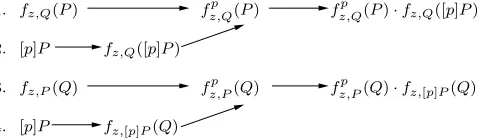
Parallelization. Figure 1 illustrates the execution path for theβ Weil pairing (6) when the four Miller functions are computed in parallel using 4 processors. As with the optimal ate pairing, Lemma 3 was repeatedly applied to each Miller function in theβWeil pairing in order to obtain a parallel implementation using 8 processors.
fz,Q(P)
[p]P
fz,P(Q)
[p]P
1.
2.
3.
4.
fz,Qp (P)
fz,Pp (Q)
fz,Q([p]P)
fz,[p]P(Q)
fz,Qp (P)·fz,Q([p]P)
fz,Pp (Q)·fz,[p]P(Q)
Fig. 1.Execution path for computing theβ Weil pairing for BLS12 curves on 4 processors.
5
KSS pairings
In this section, we consider the KSS curveY2=X3+ 2 defined with the param-eter selectionz=−264−261+ 246+ 212.
Extension field arithmetic for pairings with k=18. An element in Fp18
can be represented using the following towering scheme:
Fp3 =Fp[u]/(u3+ 2), Fp6 =Fp3[v]/(v2−u), Fp18 =Fp6[w]/(w3−v).
Table 5 gives the computational costs of the tower extensions field arithmetic for curves with k= 18, wherem512, i512 denote the cost of multiplication and inversion in Fp, with p a 512-bit prime. Moreover, ˆm, ˆs, ˆı denote the cost of
multiplication, squaring and inversion inFp3 respectively.
Computation of the optimal ate pairing. For the parameter selectionz=
−264−251+ 246+ 212, the Miller loop executes 64 point doublings with line eval-uations, 4 point additions with line evaleval-uations, 67 sparse multiplications and 63 squarings inFp18. We obtain a KSS Miller loop cost of 64(3 ˆm+ 6ˆs+ 6m512) +
4(11 ˆm+2ˆs+6m512)+67(13 ˆm)+63(11 ˆm) = 1800 ˆm+392ˆs+408m512= 13168m512. Furthermore, the final step executes 1 squaring in Fp18, one p-power
Frobe-nius, 1 multiplication inFp18, 2 point additions with line evaluation, one point
Field Mult. Squaring Inversion
Fp3 mˆ = 6m512 sˆ= 5m512 ˆı= 12m512+i512
Fp6 3 ˆm 2 ˆm 2 ˆm+ 2ˆs+ ˆı
Fp18 18 ˆm 11 ˆm 20 ˆm+ 8ˆs+ ˆı
Gφ6(Fp3) 18 ˆm 6 ˆm Conjugation
Operation Cost
Sparse Mult. 13 ˆm Sparser Mult. 7 ˆm Compressed Squaring 4 ˆm Simult. decompression n(3 ˆm+ 3ˆs)+
ofnfield elements (n−1)3 ˆm+ ˆı p-th Frobenius 15m
Table 5. Costs of arithmetic operations in a tower extension fieldFp18.
and the computation of the isomorphism ψ(Q). Thus the KSS final step cost is 11 ˆm+ 18 ˆm + 2(11 ˆm + 2ˆs+ 6m512) + 3 ˆm+ 6ˆs+ 6m512 + 20 ˆm + 28m512 = 74 ˆm+ 10ˆs+ 40m512 = 534m512. The final exponentiation executes in to-tal one inversion in Fp18, 8 cyclotomic squarings, 54 multiplications inFp18, 29
p-power Frobenius, and 7 exponentiations byz [11]. The computational cost of an exponentiation byz is 64 compressed squarings, decompression of 4 field el-ements and 3 multiplications inFp18, for a total cost of 64(6ˆs) + 4(3ˆs+ 3 ˆm) +
9 ˆm+ ˆı+ 3(18 ˆm) = 75 ˆm+ 396ˆs+ ˆı. Hence, the total cost of the final expo-nentiation is 20 ˆm+ 8ˆs+ ˆı+ 8(6 ˆm) + 54(18 ˆm) + 435m512+ 7(75 ˆm+ 396ˆs+ ˆı) = 1565 ˆm+2780ˆs+8ˆı+435m512= 23821m512+8i512Finally, the total cost of com-puting the KSS optimal ate pairing is 13168m512+534m512+23821m512+8i512= 37523m512+ 8i512.
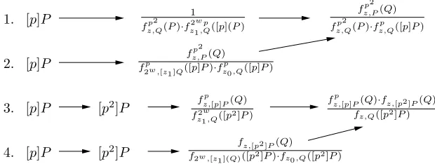
Computation of the β Weil pairing. The most expensive part of the β Weil pairing for KSS curves (4) are the six Miller functions fz,R. For parallel
implementation using 4 cores, repeated applications of Lemma 3 can be used to writez= 2wz
1+z0 such thatfz,Rcan be computed in the following way:
fz,R=f2
w
z1,R·f2w,[z1]R·fz0,R·(ℓ2w·[z1]R,[z0]R)/v[z]R.
For the KSS parameter z = −264 −251+ 246+ 212, we chose w = 36, z 1 =
−228+ 215+ 210, z
0 = 212 and split the two most expensive Miller functions fz,Qp ([p]P) andfz,Q([p2]P). Figure 2 illustrates an execution path. At the end, it
is necessary for each core to compute the additional functions (f3p,R·ℓ[z]R,[3p]R)p
i
and the exponentiation by (p9−1)·(p3+ 1).
3. [p]P [p2]P 1. [p]P
2. [p]P
4. [p]P [p2]P
1
fz,Qp2 (P)·fz2w p 1,Q([p](P)
fz,Pp2 (Q)
fz,Qp2 (P)·fz,Qp ([p]P)
fz,Pp2(Q)
fp
2w ,[z1 ]Q([p]P)·f p z0,Q([p]P)
fz,p[p]P(Q)·fz,[p2 ]P(Q)
fz,Q([p2]P)
fz,[p2 ]P(Q)
f2w ,[z1 ](Q)([p2]P)·fz0,Q([p2]P)
fz,p[p]P(Q)
f2w z1,Q([p2]P)
Fig. 2. Execution path for computing the β Weil pairing for KSS curves on 4 processors.
6
BN pairings
In this section, we consider the BN curveY2=X3+5 defined with the parameter selectionz= 2158−2128−268+ 1. The extension fields areF
p2 =Fp[u]/(u2+ 1), Fp6 =Fp2[v]/(v3−ξ) withξ=u+ 2, andFp12 =Fp6[w]/(w2−v).
Computation of the optimal ate pairing. The Miller loop executes 160 point doublings with line evaluations, 6 point additions with line evaluations, 164 sparse multiplications, 1 sparser multiplication and 159 squarings in Fp12.
We obtain a BN Miller loop cost of 160(3 ˜m+6˜s+4m640)+6(11 ˜m+2˜s+4m640)+ 164(13 ˜m) + 7 ˜m+ 159(12 ˜m) = 4593 ˜m+ 972˜s+ 664m640= 16387m640.
Furthermore, the final step executes ψ(Q), ψ2(Q), 2 point additions with line evaluation, 1 sparser multiplication and 1 multiplication in Fp12. The p-th
power Frobenius can be computed at a cost of about 5m640and thep2-th power Frobenius can be computed at a cost of about 4m640. Thus the BN final step cost is 2(11 ˜m+2˜s+4m640)+7 ˜m+18 ˜m+9m640= 47 ˜m+4˜s+17m640= 166m640. The final exponentiation executes in total 1 inversion inFp12, 3 cyclotomic squarings,
12 multiplications inFp12, 2 p-th power Frobenius, 1p2-th power Frobenius, 1
p3-th power Frobenius, and 3 exponentiations byz[11]. The computational cost of an exponentiation by z is: 158 compressed squarings, decompression of 3 field elements and 3 multiplications inFp12, for a total cost of 158(6˜s) + 3(3˜s+
3 ˜m) + 6 ˜m+ ˜ı+ 3(18 ˜m) = 69 ˜m+ 957˜s+ ˜ı. Hence, the total cost of the final exponentiation is 23 ˜m+ 11˜s+ ˜ı+ 3(9˜s) + 12(18 ˜m) + 50m640+ 3(69 ˜m+ 957˜s+ ˜ı) = 446 ˜m+ 2909˜s+ 62m640+ 4i640= 7218m640+ 4i640. Finally, the total cost of computing the BN optimal ate pairing is 16387m640+ 166m640+ 7218m640+ 4i640= 23771m640+ 4i640.
7
BLS24 pairings
In this section, we consider the BLS24 curve Y2 = X3+ 1 defined with the parameter selectionz=−248+ 245+ 231−27.
Extension field arithmetic for pairings with k=24. An element in Fp24
can be represented using the following towering scheme:
Fp2 =Fp[i]/(i2+ 1),
Fp4 =Fp2[u]/(u2−ξ), withξ=i+ 1, Fp12 =Fp4[v]/(v3−u),
Fp24 =Fp12[w]/(w2−v).
Table 6 gives the computational costs of the tower extension field arithmetic for curves with k= 24, where m480 and i480 denote the cost of multiplication and inversion in Fp, with p a 479-bit prime. Moreover, ˜m, ˜s, ˜ı denote the cost of
multiplication, squaring and inversion inFp2 respectively.
Field Mult. Squaring Inversion
Fp2 m˜ = 3m480 s˜= 2m480 ˜ı= 4m480+i480
Fp4 3 ˜m 2 ˜m 2 ˜m+ 2˜s+ ˜ı
Fp12 18 ˜m 12 ˜m 23 ˜m+ 11˜s+ ˜ı Fp24 54 ˜m 36 ˜m 83 ˜m+ 11˜s+ ˜ı Gφ6(Fp4) 54 ˜m 18 ˜m Conjugation
Operation Count Sparse Mult. 39 ˜m Sparser Mult. 21 ˜m Compressed Squaring 12 ˜m
Simult. decompression (2n−1)(9 ˜m) +n(6 ˜m) ofnfield elements +2 ˜m+ 2˜s+ ˜ı
p-th Frobenius 45m
Table 6. Costs of arithmetic operations in a tower extension fieldFp24.
Computation of the optimal ate pairing.The Miller loop executes 48 point doublings with line evaluations, 4 point additions with line evaluations, 51 sparse multiplications and 47 squarings inFp24. We obtain a BLS24 Miller loop cost of
48(21 ˜m+ 8m480) + 4(37 ˜m+ 8m480) + 51(39 ˜m) + 47(36 ˜m) = 4837 ˜m+ 416m480= 14927m480. The computation of the final exponentiation requires 1 inversion, 9 exponentiations byz, 14 multiplications inFp24, 2 cyclotomic squarings, and 8
Hence, the total cost of the final exponentiation is (83 ˜m+ 11˜s+ ˜ı) + 9(827 ˜m+ 2˜s+ ˜ı) + 14(54 ˜m) + 2(18 ˜m) + 360m480 = 8318 ˜m+ 29˜s+ 400m480+ 10i480 = 25412m480+ 10i480. Finally, the total cost of computing the BLS24 optimal ate pairing is 14927m480+ 25412m480+ 10i480= 40339m480+ 10i480.
Computation of the β Weil pairing. Since 8|ewhere e=k/d, the paral-lelization procedure for the β Weil pairing (7) on 2, 4 and 8 cores is straight-forward: with 2 cores, each core computes 4 Miller functions; with 4 cores, each core computes 2 Miller functions; and with 8 cores: each core computes 1 Miller function.
8
Comparisons
Estimates for serial implementations of the optimal ate pairings.The customary way to estimate the cost of a pairing is to count multiplications in the underlying finite fields. Notice that in the case of software implementations in modern desktop platforms, field elements a ∈ Fp can be represented with
ℓ = 1 +⌊log2(p)⌋ binary coefficientsai packed in n64 =⌈64ℓ⌉ 64-bit processor words. If Montgomery representation is used to implement field multiplication in
Fp640 andFp512 with complexityO(2n
2
64+n64), then it is reasonable to estimate that we havem640≈(210/136)·m512≈1.544·m512.
Table 7 summarizes the costs in terms of finite field multiplications for com-puting the optimal ate pairing over our choice of KSS, BN, BLS12 and BLS24 curves at the 192-bit security level.3 As can be seen, our estimates predict that the optimal ate pairing over BLS12 curves is the most efficient choice at the 192-bit security level, with KSS, BN and BLS24 curves being significantly slower. The main computational bottleneck for BLS24 curves is their very expensive final exponentiation.
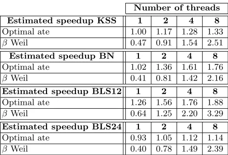
Estimates for multi-core implementations of the optimal ate and β
Weil pairings. Table 8 (see also Figure 3) shows estimated speedups for the parallel version of the optimal ate pairing using the partitions in Table 9 and all the β Weil pairing variants considered here. All speedup factors are with respect to the serial version of the KSS optimal ate pairing. It can be seen that the estimated performance for BLS12 curves when using 8 cores is of a factor-3.29 acceleration, which is the highest speedup we obtain. Perhaps the most notable observation from Table 8 is that, for eight-core implementations, the β Weil pairing becomes more efficient than the optimal ate pairing for all the four curves considered.
Curve Phase Mult. inFp Mult. inFp512
Miller Loop 13168m512 13168m512 KSS Final Step 534m512 534m512
Final Exp. 23821m512 23821m512 ML + FS + FE 37523m512 37523m512 Miller Loop 16387m640 25301m512 BN Final Step 166m640 256m512
Final Exp. 7218m640 11145m512 ML + FS + FE 23771m640 36702m512 Miller Loop 10865m640 16775m512 BLS12 Final Exp. 8464m640 13068m512 ML + FE 19329m640 29843m512 Miller Loop 14927m480 14927m512 BLS24 Final Exp. 25412m480 25412m512 ML + FE 40339m480 40339m512
Table 7. Cost estimates of the optimal ate pairing for KSS, BN, BLS12 and BLS24 curves at the 192-bit security level. Note that m480 =m512 in a 64-bit processor.
Number of threads
Estimated speedup KSS 1 2 4 8
Optimal ate 1.00 1.17 1.28 1.33 βWeil 0.47 0.91 1.54 2.51
Estimated speedup BN 1 2 4 8
Optimal ate 1.02 1.36 1.61 1.76 βWeil 0.41 0.81 1.42 2.16
Estimated speedup BLS12 1 2 4 8
Optimal ate 1.26 1.56 1.76 1.88 βWeil 0.64 1.25 2.20 3.29
Estimated speedup BLS24 1 2 4 8
Optimal ate 0.93 1.05 1.12 1.14 βWeil 0.40 0.78 1.49 2.39
1 2 3 4 5 6 7 8 0.9
1 1.1 1.2 1.3 1.4 1.5 1.6 1.7 1.8 1.9
number of cores
expected speedup
BLS12 BN KSS BLS24
Fig. 3.Expected speedups for KSS, BN, BLS12 and BLS24 optimal ate pairings at the 192-bit security level. All speedup factors are with respect to the serial version of the KSS optimal ate pairing.
Number of threads (c)
Curve 2 4 8
KSS 36 54, 39, 21 63, 58, 52, 45, 36, 26, 14 BN 86 129, 93, 50 149, 137, 122, 105, 85, 61, 33 BLS12 57 85, 61, 33 98, 90, 81, 70, 56, 40, 21 BLS24 26 38, 28, 15 44, 41, 37, 32, 26, 19, 10
Table 9.Parameterswi, 0< i < c, which define the partition of the forms=
2wc−1s
was implemented in the C programming language. The GCC 4.7.0 compiler suite was used with compilation flags for loop unrolling, inlining of small functions to reduce function call overheads, and optimization level-O3. The implementation was done on top of the RELIC cryptographic toolkit [1]. The code will eventually be incorporated into the library.
Them640≈1.544·m512 estimate used above was experimentally confirmed with carefully crafted Assembly code for multiplication and Montgomery reduc-tion. Implementing the double-precision arithmetic needed for efficient applica-tion of lazy reducapplica-tion proved to be slightly cumbersome due to the exhausapplica-tion of the 16 general-purpose registers available in the target platform (one of the regis-ters is mostly reserved for keeping track of stack memory, aggravating the effect). Naturally, this issue had a bigger performance impact on the larger 638-bit field, introducing higher penalties for reading and writing values stored into memory. By using a very efficient implementation of the Extended Euclidean Algorithm imported from the GMP4 library, we obtained inversion-to-multiplication ratios inFpof around 16, suggesting the use of the projective coordinate system instead
of the affine coordinates recommended in [28] and [20], even after considering the action of the norm map to simplify the inversion operation in extension fields. Affine coordinates were only competitive for the BLS24 curve.
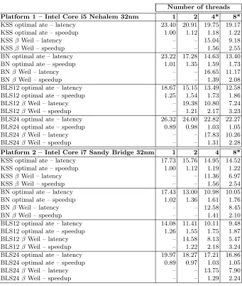
The resulting timings for the two platforms are presented in Table 10 (mea-sured with the Turbo Boost feature disabled). Timings for the parallel imple-mentation of pairings which were estimated to be slower than the reference performance of the KSS pairing are omitted. We obtained results confirming our performance estimates, i.e., the BLS12 curve is the most efficient choice for pair-ing computation at the 192-bit security level across all the considered scenarios. In particular, our fastest serial implementation on the Intel Core i5 Nehalem machine can compute a pairing in approximately 19 million cycles, more than 3 times faster than the current state-of-the-art. The previous speed record for a single pairing computation without precomputation at this security level was presented in [28, Table 2, column 4 halved] and achieves a latency of 60 million cycles on a very similar machine when a factor of 1.22 is applied to the timings to adjust for the effect of Turbo Boost.5 Additionally, theβ Weil pairing presents itself as the most efficient and scalable choice of pairing in a multiprocessor machine with more than 4 processing units.
References
1. D. F. Aranha, C. P. L. Gouvˆea, RELIC is an Efficient LIbrary for Cryptography, http://code.google.com/p/relic-toolkit/.
2. D. F. Aranha, K. Karabina, P. Longa, C. Gebotys and J. L´opez, “Faster explicit formulas for computing pairings over ordinary curves”,Advances in Cryptology – EUROCRYPT 2011, LNCS 6632 (2011), 48–68.
4
GNU Multiple Precision Arithmetic Library: http://www.gmplib.org 5
Number of threads
Platform 1 – Intel Core i5 Nehalem 32nm 1 2 4* 8*
KSS optimal ate – latency 23.40 20.91 19.75 19.17 KSS optimal ate – speedup 1.00 1.12 1.18 1.22
KSSβWeil – latency – – 15.04 9.18
KSSβWeil – speedup – – 1.56 2.55
BN optimal ate – latency 23.22 17.28 14.63 13.40 BN optimal ate – speedup 1.01 1.35 1.59 1.73
BNβWeil – latency – – 16.65 11.17
BNβWeil – speedup – – 1.39 2.08
BLS12 optimal ate – latency 18.67 15.15 13.49 12.58 BLS12 optimal ate – speedup 1.25 1.54 1.73 1.86
BLS12β Weil – latency – 19.38 10.80 7.24
BLS12β Weil – speedup – 1.21 2.17 3.23
BLS24 optimal ate – latency 26.32 24.00 22.82 22.27 BLS24 optimal ate – speedup 0.89 0.98 1.03 1.05
BLS24β Weil – latency – – 17.83 10.26
BLS24β Weil – speedup – – 1.31 2.28
Platform 2 – Intel Core i7 Sandy Bridge 32nm 1 2 4 8*
KSS optimal ate – latency 17.73 15.76 14.95 14.52 KSS optimal ate – speedup 1.00 1.12 1.19 1.22
KSSβWeil – latency – – 11.36 6.97
KSSβWeil – speedup – – 1.56 2.54
BN optimal ate – latency 17.43 13.00 10.98 10.05 BN optimal ate – speedup 1.02 1.36 1.61 1.76
BNβWeil – latency – – 12.58 8.45
BNβWeil – speedup – – 1.41 2.10
BLS12 optimal ate – latency 14.08 11.41 10.11 9.48 BLS12 optimal ate – speedup 1.26 1.55 1.75 1.87
BLS12β Weil – latency – 14.58 8.13 5.47
BLS12β Weil – speedup – 1.22 2.18 3.24
BLS24 optimal ate – latency 19.97 18.27 17.21 16.86 BLS24 optimal ate – speedup 0.89 0.97 1.03 1.05
BLS24β Weil – latency – – 13.75 7.90
BLS24β Weil – speedup – – 1.29 2.24
3. D. F. Aranha, E. Knapp, A. Menezes and F. Rodr´ıguez-Henr´ıquez. “Parallelizing the Weil and Tate pairings”, Cryptography and Coding, LNCS 7089 (2011), 275– 295.
4. D. F. Aranha, J. L´opez and D. Hankerson, “High-speed parallel software imple-mentation of the ηT pairing”,Topics in Cryptology – CT-RSA 2010, LNCS 5985 (2010), 89–105.
5. P. Barreto, H. Kim, B. Lynn and M. Scott, “Efficient algorithms for pairing-based cryptosystems”, Advances in Cryptology – CRYPTO 2002, LNCS 2442 (2002), 354–368.
6. P. Barreto, B. Lynn and M. Scott, “Constructing elliptic curves with prescribed embedding degrees”, Security in Communication Networks – SCN 2002, LNCS 2576 (2003), 257–267.
7. P. Barreto and M. Naehrig, “Pairing-friendly elliptic curves of prime order”, Se-lected Areas in Cryptography – SAC 2005, LNCS 3897 (2006), 319–331.
8. F. Brezing and A. Weng, “Elliptic curves suitable for pairing based cryptography”, Designs, Codes and Cryptography, 37 (2006), 133–141.
9. C. Costello, K. Lauter and M. Naehrig, “Attractive subfamilies of BLS curves for implementing high-security pairings”, Progress in Cryptology – INDOCRYPT 2011, LNCS 7107 (2011), 320–342.
10. D. Freeman, M. Scott and E. Teske, “A taxonomy of pairing-friendly elliptic curves”,Journal of Cryptology, 23 (2010), 224–280.
11. L. Fuentes-Casta˜neda, E. Knapp and F. Rodr´ıguez-Henr´ıquez, “Faster hashing to
G2”,Selected Areas in Cryptography – SAC 2011, LNCS 7118 (2012), 412-430. 12. S. Galbraith, K. Harrison and D. Soldera, “Implementing the Tate pairing”,
Algo-rithmic Number Theory – ANTS 2002, LNCS 2369 (2002), 324–337.
13. S. Galbraith, K. Paterson and N. Smart, “Pairings for cryptographers”, Discrete Applied Mathematics, 156 (2008), 3113–3121.
14. R. Granger, F. Hess, R. Oyono, N. Th´eriault and F. Vercauteren, “Ate pairing on hyperelliptic curves”, Advances in Cryptology – EUROCRYPT 2007, LNCS 4515 (2007), 430–447.
15. F. Hess, “Pairing lattices”, Pairing-Based Cryptography – Pairing 2008, LNCS 5209 (2008), 18–38.
16. F. Hess, N. Smart and F. Vercauteren, “The eta pairing revisited”IEEE Transac-tions on Information Theory, 52 (2006), 4595–4602.
17. E. Kachisa, E. Schaefer and M. Scott, “Constructing Brezing-Weng pairing-friendly elliptic curves using elements in the cyclotomic field”,Pairing-Based Cryptography – Pairing 2008, LNCS 5209 (2008), 126–135.
18. K. Karabina, “Squaring in cyclotomic subgroups”,Mathematics of Computation, to appear.
19. N. Koblitz and A. Menezes, “Pairing-based cryptography at high security levels”, Cryptography and Coding, LNCS 3796 (2005), 13–36.
20. K. Lauter, P. Montgomery and M. Naehrig, “An analysis of affine coordinates for pairing computation”, Pairing-Based Cryptography – Pairing 2010, LNCS 6487 (2010), 1–20.
21. A. Lenstra, H. Lenstra and L. Lovasz, “Factoring polynomials with rational coef-ficients”,Mathematische Annalen, 261 (1982) 515–534.
22. V. Miller, “The Weil pairing, and its efficient calculation’,Journal of Cryptology, 17 (2004), 235–261.
24. G. Pereira, M. Simpl´ıcio Jr., M. Naehrig and P. Barreto, “A family of implementation-friendly BN elliptic curves”,Journal of Systems and Software, 84 (2011), 1319–1326.
25. J. Pollard, “Monte Carlo methods for index computation modp”,Mathematics of Computation, 32 (1978), 918–924.
26. O. Schirokauer, “Discrete logarithms and local units”,Philosophical Transactions of the Royal Society London A, 345 (1993), 409–423.
27. M. Scott, “Computing the Tate pairing”,Topics in Cryptology — CT-RSA 2005, LNCS 3376 (2005) 300–312.
28. M. Scott, “On the efficient implementation of pairing-based protocols”, Cryptog-raphy and Coding, LNCS 7089 (2011), 296–308.
29. M. Scott, N. Benger, M. Charlemagne, L. J. Dominguez-Perez and E. J. Kachisa, “On the final exponentiation for calculating pairings on ordinary elliptic curves”, Pairing-Based Cryptography – Pairing 2009, LNCS 5671 (2009), 78–88.
![Table 1 summarizes the salient parameters of the KSS [17], BN [7], BLS12 [6]](https://thumb-us.123doks.com/thumbv2/123dok_us/7890982.1309523/3.612.148.469.432.496/table-summarizes-salient-parameters-kss-bn-bls.webp)