Volume 2007, Article ID 86484,19pages doi:10.1155/2007/86484
Research Article
Underdetermined Blind Source Separation in Echoic
Environments Using DESPRIT
Thomas Melia and Scott Rickard
Sparse Signal Processing Group, University College Dublin, Belfield, Dublin 4, Ireland
Received 1 October 2005; Revised 4 April 2006; Accepted 27 May 2006 Recommended by Andrzej Cichocki
The DUET blind source separation algorithm can demix an arbitrary number of speech signals usingM=2 anechoic mixtures of the signals. DUET however is limited in that it relies upon source signals which are mixed in an anechoic environment and which are sufficiently sparse such that it is assumed that only one source is active at a given time frequency point. The DUET-ESPRIT (DESPRIT) blind source separation algorithm extends DUET to situations whereM≥2 sparsely echoic mixtures of an arbitrary number of sources overlap in time frequency. This paper outlines the development of the DESPRIT method and demonstrates its properties through various experiments conducted on synthetic and real world mixtures.
Copyright © 2007 T. Melia and S. Rickard. This is an open access article distributed under the Creative Commons Attribution License, which permits unrestricted use, distribution, and reproduction in any medium, provided the original work is properly cited.
1. INTRODUCTION
The “cocktail party phenomenon” illustrates the ability of the human auditory system to separate out a single speech source from the cacophony of a crowded room using only two sensors with no prior knowledge of the speakers or the channel presented by the room. Efforts to implement a re-ceiver which emulates this sophistication are referred to as blind source separation techniques [1–3]. The DUET blind source separation method [4] can demix an arbitrary num-ber of speech source signals given just 2 anechoic mixtures of the sources, providing that the time-frequency representa-tions of the sources do not overlap. The technique is limited in the following respects.
(1) It is not obvious how to best extend the technique to a situation where more mixtures are available.
(2) The assumption that only one source is active at a given time-frequency point is limiting, especially when M >2 mixtures may be available.
(3) The anechoic mixing model clearly restricts the types of environments where DUET can be applied. A number of extensions to the DUET blind source separa-tion method have recently been proposed [5–7] that address these issues. In this paper we summarise and characterise the performance of these extensions, which we believe em-body the natural multichannel, echoic extension of DUET. Other authors have proposed different DUET extensions, for
example, [8–11] describe multichannel extensions to DUET whenM ≥ 2 mixtures are available. It is recognised in [9– 15] that the assumption that only one source is active at a given time-frequency point is quite a harsh restriction to place upon large numbers of speech sources and weakened forms of this assumption are presented in these papers. An echoic extension to DUET is demonstrated in [9] when the mixing parameters are known a priori. In this work, we ex-tend DUET to useM >2 mixtures and in doing so are able to separate multiple sources at each time-frequency point, even when mixing is echoic.
In general, we seek to demixMmixtures ofNsource sig-nals taken from a uniform linear array of sensors. In the fre-quency domain we model theMmixturesX1(ω),. . .,XM(ω)
ofNsource signalsS1(ω),. . .,SN(ω) as ⎡
⎢ ⎢ ⎢ ⎢ ⎣
X1(ω)
X2(ω)
.. . XM(ω)
⎤ ⎥ ⎥ ⎥ ⎥
⎦=
⎡ ⎢ ⎢ ⎢ ⎢ ⎣
1 · · · 1
φ1(ω) · · · φN(ω)
..
. ...
φM−1
1 (ω) · · · φNM−1(ω)
⎤ ⎥ ⎥ ⎥ ⎥ ⎦ ⎡ ⎢ ⎢ ⎣
A1(ω)S1(ω)
.. . AN(ω)SN(ω)
⎤ ⎥ ⎥ ⎦
+
⎡ ⎢ ⎢ ⎢ ⎢ ⎣
V1(ω)
V2(ω)
.. . VM(ω)
⎤ ⎥ ⎥ ⎥ ⎥ ⎦,
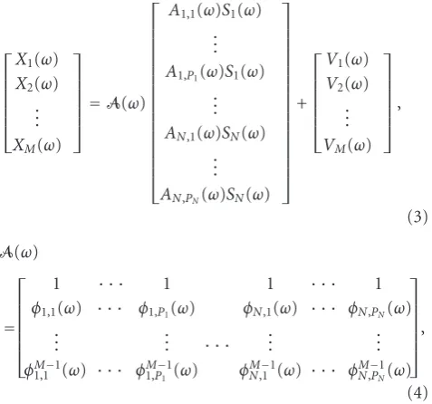
whereAn(ω)=ane−jωdn,ananddnare the attenuation and delay experienced by thenth signal as it propagates to the 1st sensor,φn(ω)=αne−jωδn,αnandδnare the attenuation and delay experienced by thenth signal as it travels between two adjacent sensors, andV1(ω),V2(ω),. . .,VM(ω) are
indepen-dently and identically distributed noise terms. Equivalently in the time domain themth anechoic mixturexm(t) of theN source signals,s1(t),s2(t),. . .,sN(t), can be expressed as
xm(t)= N
n=1
anαmn−1sn t−dn−(m−1)δn
+vm(t), (2)
where the inverse Fourier transform is defined as f(t) = (1/2π)−∞∞ F(ω)ejωtdω. The anechoic mixing model (1) may be altered to become an echoic mixing model by adding columns to the mixing matrix corresponding to echoic paths:
⎡ ⎢ ⎢ ⎢ ⎢ ⎢ ⎣
X1(ω)
X2(ω)
.. . XM(ω)
⎤ ⎥ ⎥ ⎥ ⎥ ⎥
⎦=A(ω) ⎡ ⎢ ⎢ ⎢ ⎢ ⎢ ⎢ ⎢ ⎢ ⎢ ⎢ ⎢ ⎢ ⎢ ⎢ ⎢ ⎢ ⎣
A1,1(ω)S1(ω)
.. . A1,P1(ω)S1(ω)
.. . AN,1(ω)SN(ω)
.. . AN,PN(ω)SN(ω)
⎤ ⎥ ⎥ ⎥ ⎥ ⎥ ⎥ ⎥ ⎥ ⎥ ⎥ ⎥ ⎥ ⎥ ⎥ ⎥ ⎥ ⎦
+
⎡ ⎢ ⎢ ⎢ ⎢ ⎢ ⎣
V1(ω)
V2(ω)
.. . VM(ω)
⎤ ⎥ ⎥ ⎥ ⎥ ⎥ ⎦,
(3)
A(ω)
= ⎡ ⎢ ⎢ ⎢ ⎢ ⎢ ⎣
1 · · · 1 1 · · · 1
φ1,1(ω) · · · φ1,P1(ω) φN,1(ω) · · · φN,PN(ω) ..
. ... · · · ... ...
φM−1
1,1 (ω) · · · φM1,P−11(ω) φ
M−1
N,1 (ω) · · · φNM,−PN1(ω) ⎤ ⎥ ⎥ ⎥ ⎥ ⎥ ⎦,
(4)
whereAn,p(ω)=an,pe−jωdn,p,an,panddn,pare the attenuation and delay experienced by thenth signal as it propagates along itspth path, to the 1st sensor,φn,p(ω)=αn,pe−jωδn,p,αn,pand δn,pare the attenuation and delay experienced by thenth sig-nal as it propagates between two adjacent sensors along its pth path andPnis the number of paths thenth source sig-nal travels upon to reach the sensor array. Equivalently in the time domain themth echoic mixture can be expressed as
xm(t)= N
n=1
Pn
p=1
an,pαmn,−p1sn t−dn,p−(m−1)δn,p
+vm(t).
(5)
This model has the same form as (1) but now there are N ≥ N signals being received by the sensor array, some of these signals will be originated from the same source. Figure 1illustrates a simple anechoic mixing procedure and a related echoic mixing procedure. Our treatment assumes a uniform linear array with spacing≤ c/2fmax throughout,
where fmax is the maximum frequency of interest and cis
the speed at which the signals propagate. Furthermore it is
s1(t)
s2(t) s3(t)
x1(t) x2(t) x3(t)
(a)
s1(t)
s1(t) s2(t)
x1(t) x2(t) x3(t)
(b)
Figure1: 3 sensors pick up 3 anechoic mixtures of 3 signals (a) and 3 echoic mixtures of 2 signals (b).
assumed that the sensor array is located sufficiently far away from the source locations that planar wave propagation oc-curs, although not previously stated, this assumption is im-plicit in the mixing models (1) and (3).
The goal of a blind source separation method is to estimate the source signals s1(t),s2(t),. . .,sN(t) from the
mixture signals x1(t),x2(t),. . .,xM(t). This paper describes
the significant power containing coefficients for two differ-ent speech signals rarely overlap. This leads to the W-disjoint orthogonal (WDO) property [4]
Sn(ω,τ)Sl(ω,τ)=0 ∀ω,τ,n=l, (6)
where the time-frequency representation of the signalsn(t) is given by the windowed Fourier transform
Sn(ω,τ)=
∞
−∞W(t−τ)sn(t)e
−jωtdt, (7)
whereW(t) is a window function. Note that this is a math-ematical idealisation and in practice it is sufficient that |Sn(ω,τ)Sl(ω,τ)|be small with high probability [4,8]. The DUET algorithm uses this assumption to separateNspeech signals from one anechoic mixture of the signals by par-titioning the time-frequency plane. In order to determine the demixing partitions, DUET uses two mixtures:x1(t) and
x2(t). For simplicity consider the case whereW(t) = 1, in
which case the system model (1) becomes
X1(ω)
X2(ω)
=
1 · · · 1
α1e−jωδ1 · · · αNe−jωδN ⎡⎢
⎢ ⎢ ⎣
A1(ω)S1(ω)
.. . AN(ω)SN(ω)
⎤ ⎥ ⎥ ⎥ ⎦
+
V1(ω)
V2(ω)
.
(8)
As the planar wave from thenth sourcesn(t) travels across the two-element array, the signal seen by the first sensor is attenuated or amplified by a real scalar,αn, and delayed byδn seconds before it reaches the second sensor. Without loss of generality theN channel coefficientsA1(ω),. . .,AN(ω) can
be absorbed by theNsource signals, that is,An(ω)Sn(ω)→ Sn(ω), n = 1,. . .,N. In the no-noise case, with W-disjoint orthogonal sources, the two mixtures of the sources are re-lated to at most one of the source signals at any given point in the frequency domain. That is
⎡ ⎣X1(ω)
X2(ω) ⎤
⎦=
1
αne−jωδn Sn(ω)
(9)
for a given value of frequencyω∈Ωn, where
Ωn=
ω:Sn(ω)=0 (10)
defines the support ofSn(ω). For such values ofω, the atten-uation and delay parameters for thenth source can be deter-mined by
αn=X2(ω)
X1(ω)
, δn= −1
ω∠
X2(ω)
X1(ω)
, (11)
where∠{αejβ} =β. Scanning acrossωin the support of the mixtures, (11) will take onNdistinct attenuation and delay value pairings; theseNpairings are the mixing parameters. When noise is present, (11) will be approximately satisfied
and a two-dimensional histogram in attenuation-delay space constructed using (11) will containN peaks, one for each source, with peak locations corresponding to the mixing pa-rameters. Labelling eachωwith the peak its corresponding amplitude-delay estimate falls closest to, we partition one of the mixtures in the frequency domain into the original source signals.
Using the narrowband assumption in the time-frequency domain, that is, ifs1(t)=s(t) ands2(t)=s(t−δ) then for all
δ <Δmax,
S2(ω,τ)≈e−jωδS1(ω,τ) (12)
for some max delay Δmax, the expression (11) can be
ex-tended to the time-frequency domain. Neglecting the effect of noise and assuming (6) is strictly satisfied, the attenuation and delay parameters of thenth signal are then given by
αn=X2(ω,τ)
X1(ω,τ)
, δn= −1
ω∠
X2(ω,τ)
X1(ω,τ)
(13)
for (ω,τ)∈Ωn, where
Ωn=
(ω,τ) :Sn(ω,τ)=0 (14)
defines the support of Sn(ω,τ). Now, similarly scanning across (ω,τ) in the support of the mixtures, (13) will take onNdistinct attenuation and delay value pairings, the mix-ing parameters. When noise is present and (6) is approxi-mately satisfied, (13) will be approxiapproxi-mately satisfied and a two-dimensional histogram in attenuation-delay space con-structed using (13) will again containNpeaks, one for each source, with peak locations corresponding to the mixing pa-rameters. Labelling each (ω,τ) with the peak its correspond-ing amplitude-delay estimate falls closest to, one of the mix-tures is then partitioned in the time-frequency domain into the original source signals.
The remainder of this paper has the following structure. Section 2describes the classic ESPRIT direction of arrival es-timation algorithm and the development of the hard DE-SPRIT, soft DEDE-SPRIT, and echoic DESPRIT extensions to the DUET blind source separation technique.Section 3gives an algorithmic description of the echoic DESPRIT technique. Section 4describes a set of synthetic and real-room experi-ments designed to demonstrate properties and advantages of the hard DESPRIT, soft DESPRIT, and echoic DESPRIT ex-tensions to the DUET blind source separation technique.
2. THE DESPRIT TECHNIQUE
2.1. The ESPRIT direction of arrival
estimation algorithm
Classic direction of arrival estimation techniques such as MUSIC [22] and ESPRIT [23] aim to find the N angles of arrival of N uncorrelated narrowband signals s1(t),s2(t),. . .,sN(t) as they impinge onto an array ofM
x1(t)
x2(t)
(a) x1(t)
x2(t)
(b) x1(t)
x2(t)
(c)
Figure2: ESPRIT subarray separation of a uniform linear array in the case ofM=M/2,M=M−1, andM/2<M< M−1.
For narrowband signals of centre frequencyω0, a time
lag can be approximated by a phase rotation, that is, for all δ <Δmax,
s(t−δ)≈e−jω0δs(t) (15)
for some max delayΔmax, wheres(t) is the complex analytic
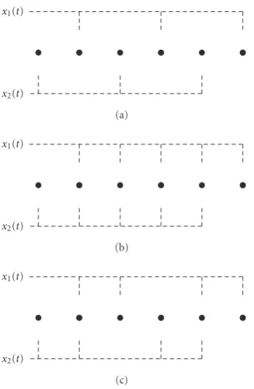
representation of real signals(t). In this section only, all func-tions of time are assumed to be in their complex analytic representation and for notational simplicity we will drop the {·}from them. ESPRIT separates theMmixtures into two subsets of M mixtures each, whereM/2 ≤ M ≤ M−1. The first subarray of M sensors must be displaced from a second identical subarray of Msensors by a common dis-placement vector. In the case of a uniform linear array (see Figure 2), the subarrays can be chosen to maximise overlap, that is,M=M−1 and the output of the first subarray may be expressed as
⎡ ⎢ ⎢ ⎢ ⎢ ⎢ ⎣
x1(t)
x2(t)
.. . xM−1(t)
⎤ ⎥ ⎥ ⎥ ⎥ ⎥ ⎦= ⎡ ⎢ ⎢ ⎢ ⎢ ⎢ ⎣
1 · · · 1
φ1 ω0
· · · φN ω0
..
. ...
φM1−2 ω0
· · · φMN−2 ω0 ⎤ ⎥ ⎥ ⎥ ⎥ ⎥ ⎦ × ⎡ ⎢ ⎢ ⎢ ⎣
A1 ω0
s1(t)
.. . AN ω0
sN(t)
⎤ ⎥ ⎥ ⎥ ⎦+ ⎡ ⎢ ⎢ ⎢ ⎢ ⎢ ⎣
v1(t)
v2(t)
.. . vM−1(t)
⎤ ⎥ ⎥ ⎥ ⎥ ⎥ ⎦ (16)
and the output of the second subarray may be expressed as
⎡ ⎢ ⎢ ⎢ ⎢ ⎢ ⎣
x2(t)
x3(t)
.. . xM(t)
⎤ ⎥ ⎥ ⎥ ⎥ ⎥ ⎦= ⎡ ⎢ ⎢ ⎢ ⎢ ⎢ ⎣
φ1 ω0
· · · φN ω0
φ2 1 ω0
· · · φ2
N ω0
..
. ...
φM−1 1 ω0
· · · φM−1
N ω0 ⎤ ⎥ ⎥ ⎥ ⎥ ⎥ ⎦ × ⎡ ⎢ ⎢ ⎢ ⎣
A1 ω0
s1(t)
.. . AN ω0
sN(t)
⎤ ⎥ ⎥ ⎥ ⎦+ ⎡ ⎢ ⎢ ⎢ ⎢ ⎢ ⎣
v2(t)
v3(t)
.. . vM(t)
⎤ ⎥ ⎥ ⎥ ⎥ ⎥ ⎦, (17)
whereφn(ω0)=αne−jω0δn, andαnandδnare the attenuation
and delay experienced by thenth signal as it travels from the first subarray to the second. Both data vectors can be stacked to form a 2(M−1)×1 time-varying vector
z(t)=
x1(t) x2(t)
=
A ω0
A ω0
Φ ω0
s(t)+v(t), (18)
where
A ω0 = ⎡ ⎢ ⎢ ⎢ ⎢ ⎢ ⎣
A1 ω0
· · · AN ω0
A1 ω0
φ1 ω0
· · · AN ω0
φN ω0
..
. ...
A1 ω0
φM−2 1 ω0
· · · AN ω0
φM−2
N ω0 ⎤ ⎥ ⎥ ⎥ ⎥ ⎥ ⎦,
Φ ω0 = ⎡ ⎢ ⎢ ⎢ ⎣
φ1 ω0
. .. φN ω0
⎤ ⎥ ⎥ ⎥ ⎦, (19)
and the entries ofv(t) are noise terms. It follows that the spa-tial covariance matrix
Rzz=. E
z(t)z(t)H (20)
is of the form
Rzz=
A ω0
A ω0
Φ ω0
Rss
A ω0
A ω0
Φ ω0
H
+Rvv, (21)
where
Rss=E
s(t)s(t)H, Rvv=E
v(t)v(t)H, (22)
andE{·}is the expectation operator. ESPRIT assumes Rss
is of full rank and thus for a high signal-to-noise ratio the singular value decomposition (SVD) ofRzzcan be computed
to give
Rzz
Es Ev Λ
0
0 Σ Es Ev
H
where Λ= ⎡ ⎢ ⎢ ⎢ ⎣
λ1+σ12
. ..
λN+σ2
N ⎤ ⎥ ⎥ ⎥ ⎦, Σ= ⎡ ⎢ ⎢ ⎢ ⎣
σN2+1
. .. σ2
2(M−1) ⎤ ⎥ ⎥ ⎥ ⎦, (24)
λ1,. . .,λN σ12,. . .,σ2(2M−1),λ1,λ2,. . .,λN are related to the
source signal powers andσ2
1,σ22,. . .,σ2(2M−1)are related to the
variance of the sensor noise. TheNcolumn vectors ofEsare associated with the singular values ofΛand they are said to span the signal subspace. The 2M−N−2 column vectors of
Evassociated with the singular values ofΣspan the nullspace of Es, which is often referred to as the noise subspace. (It is understood thatRzzand its singular value decomposition
(23) have a dependence upon the centre frequencyω0, the
notation omits reference to this variable.) It follows that for high signal-to-noise ratios there exists a nonsingular matrix
S, such that
Es=
E1 E2 ≈
A ω0
A ω0
Φ ω0
S, (25)
whereE1 andE2 are the signal subspaces corresponding to
the first and second subarrays, respectively. Providing thatE1
andE2are of rankN, the diagonal matrixΦ(ω0) is related to E†1E2via a similarity transform
E†1E2≈S−1Φ ω0
S, (26)
where [·]† denotes the Moore-Penrose pseudoinverse, a least-square solution to the nosnquare matrix inverse. The ESPRIT algorithm may be summarised in the following way.
Step 1. M narrowband mixtures x1(t),. . .,xM(t) of centre
frequency ω0 are sampled at the K adjacent time points
t1,. . .,tK, these sampled mixtures are used to construct the
data matrix z= ⎡ ⎢ ⎢ ⎢ ⎢ ⎢ ⎢ ⎢ ⎢ ⎢ ⎢ ⎢ ⎢ ⎣
x1 t1
· · · x1 tK
..
. ...
xM−1 t1
· · · xM−1 tK
x2 t1
· · · x2 tK
..
. ...
xM t1
· · · xM tK
⎤ ⎥ ⎥ ⎥ ⎥ ⎥ ⎥ ⎥ ⎥ ⎥ ⎥ ⎥ ⎥ ⎦ (27)
and an estimate of the spatial covariance matrix is computed
Rzz=zzH. (28)
Step 2. The singular value decomposition (23) is computed:
Rzz=⇒
E1 Ev1
E2 Ev2
Λ 0
0 Σ
E1 Ev1
E2 Ev2
H
(29)
(Ev1andEv2are the top and bottomM−1 rows ofEv).
Step 3. TheNmixing parameters are estimated via an eigen-value decomposition
φ1 ω0
,. . .,φN ω0
=eigsE†1E2
, (30)
where eigs{H}denotes the eigenvalues of the matrixH.
2.1.1. Simplification of ESPRIT technique
As an example we consider the no-noise mixing model
⎡ ⎢ ⎢ ⎣
x1 t1
· · · x1 tK
x2 t1
. . . x2 tK
x3 t1
. . . x3 tK ⎤ ⎥ ⎥ ⎦ = ⎡ ⎢ ⎢ ⎣ 1 1
φ1 ω0
φ2 ω0
φ2 1 ω0
φ2 2 ω0
⎤ ⎥ ⎥ ⎦
s1 t1
. . . s1 tK
s2 t1
. . . s2 tK
, (31)
the spatial covariance matrix is constructed according to Step 1:
Rzz=
⎡ ⎢ ⎢ ⎢ ⎢ ⎣
x1 t1
· · · x1 tK
x2 t1
· · · x2 tK
x2 t1
· · · x2 tK
x3 t1
· · · x3 tK ⎤ ⎥ ⎥ ⎥ ⎥ ⎦ × ⎡ ⎢ ⎢ ⎢ ⎣
x1∗ t1
x∗2 t1
x∗2 t1
x3∗ t1
..
. ... ... ... x∗1 tK
x∗2 tK
x2∗ tK
x∗3 tK ⎤ ⎥ ⎥ ⎥ ⎦ (32)
and the singular value decomposition is computed as in Step 2yielding the 2×2 signal subspace matricesE1andE2.
The mixing parameter estimatesφ1(ω0) andφ2(ω0) are then
given byStep 3
φ1 ω0
,φ2 ω0
=eigsE−11E2
. (33)
The computation of the singular value decomposition in Step 2is not strictly necessary in this case,E1andE2may be
simply replaced by
E1=
x1 t1
x1 t2
x2 t1
x2 t2
, E2=
x2 t1
x2 t2
x3 t1
x3 t2
(34)
since
x1 t1
x1 t2
x2 t1
x2 t2
−1
x2 t1
x2 t2
x3 t1
x3 t2
=
s1 t1
s1 t2
s2 t1
s2 t2
−1
1 1
φ1 ω0
φ2 ω0
−1
×
φ1 ω0
φ2 ω0
φ2 1 ω0
φ2 2 ω0
s1 t1
s1 t2
s2 t1
s2 t2
=
s1 t1
s1 t2
s2 t1
s2 t2
−1
φ1 ω0
0 0 φ2 ω0
s1 t1
s1 t2
s2 t1
s2 t2
,
wheret1andt2are two adjacent sample points. As in (26)
the mixing parameters are related to E−1
1 E2via a similarity
transform, that is,
E−1
1 E2=S−1Φ ω0
S,
S=
s1 t1
s1 t2
s2 t1
s2 t2
, Φ ω0
=
φ1 ω0
0 0 φ2 ω0
.
(36)
It follows that in general forMnoiseless mixturesStep 3may be modified to become
φ1 ω0
,. . .,φM −1 ω0
=eigsE−1 1 E2
, (37)
where
E1= ⎡ ⎢ ⎢ ⎣
x1 t1
· · · x1 tM−1
..
. ...
xM−1 t1
· · · xM−1 tM−1
⎤ ⎥ ⎥ ⎦,
E2= ⎡ ⎢ ⎢ ⎢ ⎣
x2 t1
· · · x2 tM−1
..
. ...
xM t1
· · · xM tM−1 ⎤ ⎥ ⎥ ⎥ ⎦, (38)
andt1,t2,. . .,tM−1are adjacent time samples.
It is also possible to switch the order of the matrix multi-plication, that is,
φ1 ω0
,. . .,φM −1 ω0
=eigsE2E†1
; (39)
this approach removes the restriction thatM−1 time samples are used to estimateM−1 mixing parameters, nowK≥M−1 samples may be used to estimateM−1 mixing parameters. This can be shown for theM=3 case:
E1=
x1 t1
· · · x1 tK
x2 t1
· · · x2 tK
,
E2=
x1 t1
· · · x1 tK
x2 t1
· · · x2 tK
,
E2E†1 =
x2 t1
· · · x2 tK
x3 t1
· · · x3 tK
x1 t1
· · · x1 tK
x2 t1
· · · x2 tK
†
=
φ1 ω0
φ2 ω0
φ21 ω0
φ22 ω0
s1 t1
· · · s1 tK
s2 t1
· · · s2 tK
×
s1 t1
· · · s1 tK
s2 t1
· · · s2 tK
†
1 1
φ1 ω0
φ2 ω0
−1
=
1 1
φ1 ω0
φ2 ω0
φ1 ω0
0 0 φ2 ω0
×
1 1
φ1 ω0
φ2 ω0
−1
=A ω0
Φ ω0
A−1 ω 0
,
(40)
where
A ω0
=
1 1
φ1 ω0
φ2 ω0
,
Φ ω0
=
φ1 ω0
0 0 φ2 ω0
.
(41)
Again it follows that in general forMmixturesStep 3may be modified to become
φ1 ω0
,. . .,φM −1 ω0
=eigsE2E†1
, (42)
where
E1= ⎡ ⎢ ⎢ ⎢ ⎣
x1 t1
· · · x1 tK
..
. ...
xM−1 t1
· · · xM−1 tK ⎤ ⎥ ⎥ ⎥ ⎦,
E2= ⎡ ⎢ ⎢ ⎢ ⎣
x2 t1
· · · x2 tK
..
. ...
xM t1
· · · xM tK
⎤ ⎥ ⎥ ⎥ ⎦, (43)
andt1,t2,. . .,tK are adjacent time samples withK ≥ M−
1. The simplified ESPRIT algorithm may be summarised as follows.
Step 1. K≥M−1 time samples ofMnarrowband mixtures x1(t),x2(t),. . .,xM(t) are used to construct the matrices
E1= ⎡ ⎢ ⎢ ⎢ ⎣
x1 t1
. . . x1 tK
..
. ...
xM−1 t1
· · · xM−1 tK ⎤ ⎥ ⎥ ⎥ ⎦,
E2= ⎡ ⎢ ⎢ ⎢ ⎣
x2 t1
· · · x2 tK
..
. ...
xM t1
· · · xM tK
⎤ ⎥ ⎥ ⎥ ⎦. (44)
Step 2. TheM−1 mixing parameters are estimated via an eigenvalue decomposition
φ1 ω0
,. . .,φM −1 ω0
=eigsE2E†1
. (45)
2.1.2. Combining DUET and ESPRIT
TheM−1 eigenvalues obtained in (37) or in (42) serve as M−1 mixing parameter estimatesφ1(ω0),. . .,φM −1(ω0) and
theM−1 attenuation and delay estimates are then given as
αm=φm ω0,
δm= − 1 ω0∠
φm ω0
, m=1,. . .,M−1 (46)
(it may be noted that the classic ESPRIT algorithm makes the assumption that the attenuation parameters are unity, i.e., α1 = α2 = · · · = αM−1 = 1). TheM−1 delay estimates
δ1,. . .,δM −1 are related toM−1 angle of arrival estimates
θ1,. . .,θM −1onto the line of the sensor array via
δm= D c cosθm
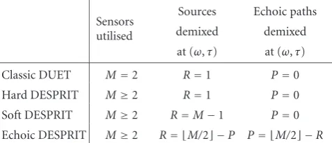
Table 1: Summary of the properties of the three extensions to DUET, where the number of echoic paths is the number of extra (nondirect) paths.
Sensors utilised
Sources Echoic paths
demixed demixed
at (ω,τ) at (ω,τ)
Classic DUET M=2 R=1 P=0
Hard DESPRIT M≥2 R=1 P=0
Soft DESPRIT M≥2 R=M−1 P=0
Echoic DESPRIT M≥2 R= M/2 −P P= M/2 −R
where c is the propagation speed and D is the array spacing. Since the attenuation and the delay estimates (α1,δ1),. . ., (αM −1,δM −1) used in the DUET algorithm to
construct the power weighted histogram are also estimated by the ESPRIT algorithm, it is possible to combine both tech-niques to form a hybrid DUET-ESPRIT technique, which is discussed in the next section. Also in adapting ES-PRIT for using with DUET, the narrowband assumption on complex analytic representations (15) is replaced with the narrowband assumption on time-frequency representations (12).
2.2. DESPRIT algorithm outline
The combined DUET-ESPRIT technique (DESPRIT) may be used to extend the DUET blind source separation algorithm to
(1) the multichannel case (M ≥2) using hard DESPRIT, discussed inSection 2.2.1,
(2) the weakened WDO case (where sources may overlap in the time-frequency domain) using soft DESPRIT, discussed inSection 2.2.2,
(3) and the echoic mixing case using echoic DESPRIT, dis-cussed inSection 2.3.
The properties of these extensions are summarised in Table 1. All three of these extensions have the same general outline.
Step 1. AnM-element uniform linear array receivesM mix-turesx1(t),x2(t),. . .,xM(t) ofNsignalss1(t),s2(t),. . .,sN(t).
TheseMmixtures are transformed into the time-frequency domain using the windowed Fourier transform.
Step 2. Centred at each sample point in the time-frequency domain, the ESPRIT algorithm is performed and the mixing parameters of the source signals active at that point are esti-mated.
Step 3. The mixing parameter estimates are used to create a weighted histogram, a technique borrowed from the DUET algorithm. The peaks of the histogram indicate sources and the centres of these peaks are used as estimates of the associ-ated mixing parameters.
Step 4. Demixing is performed by inverting a local mix-ing matrix dependent on the sources active at each time-frequency point. The resulting demixed components are partitioned and combined in a maximum-likelihood align and sum estimator using the labels from the histogram to produce the demixture time-frequency representations.
2.2.1. Hard DESPRIT: a multichannel DUET extension
The hard DESPRIT technique extends DUET to handleM > 2 mixtures but still assumes at most one source active at any time-frequency point and an anechoic mixing model. Similar to (20) the time-frequency spatial covariance matrix may be defined as
RZZ=. E
Z(ω,τ)ZH(ω,τ), (48)
where
Z(ω,τ)= ⎡ ⎢ ⎢ ⎢ ⎢ ⎢ ⎢ ⎢ ⎢ ⎢ ⎢ ⎢ ⎢ ⎢ ⎢ ⎢ ⎣
X1(ω,τ)
.. .
XM−1(ω,τ)
X2(ω,τ)
.. . XM(ω,τ)
⎤ ⎥ ⎥ ⎥ ⎥ ⎥ ⎥ ⎥ ⎥ ⎥ ⎥ ⎥ ⎥ ⎥ ⎥ ⎥ ⎦
(49)
andXm(ω,τ)=−∞∞ W(t−τ)xm(t)e−jωtdt. (Again it is under-stood thatRZZand its singular value decomposition have a
dependence upon the time-frequency point (ω,τ), the nota-tion omits reference to these variables.) Under a strong WDO assumption (6) only one source signal is active at each time-frequency point, as a resultRZZis at most rank one and has a
singular value decomposition of the form
RZZ= ⎡ ⎢ ⎣E1
E2 ⎤ ⎥ ⎦
2(M−1)×1
EH
1 EH2
1×2(M−1). (50)
It follows that
φn(ω,τ)=E†1E2 ∀(ω,τ)∈Ωn (51) is a complex scalar corresponding to the estimated mixing parameter of thenth source signal. Furthermore when the expectation operator E{·}is approximated using an instan-taneous estimate,φn (ω,τ) is given by
φn(ω,τ)=X1(ω,τ)
†
X2(ω,τ)
∀(ω,τ)∈Ωn, (52) whereX1(ω,τ) = [X1(ω,τ),. . .,XM−1(ω,τ)]T andX2(ω,τ)
=[X2(ω,τ),. . .,XM(ω,τ)]T, this expression may be restated
as
φn(ω,τ)=
M−1
m Xm∗(ω,τ)Xm+1(ω,τ) M−1
m Xm∗(ω,τ)Xm(ω,τ)
∀(ω,τ)∈Ωn.
(53)
2.2.2. Soft DESPRIT: the weakened WDO assumption
The soft DESPRIT technique extends DUET to handleM >2 mixtures and also allows for more than one source to be ac-tive at a given time-frequency point. It assumes, as DUET and hard DESPRIT do, anechoic mixing. Soft DESPRIT is an implementation of DESPRIT under a weakened WDO as-sumption [6]:
Sn1(ω,τ)× · · · ×SnM(ω,τ)=0 ∀ω,τ,nl=nk,l=k. (54)
This weakened WDO assumption allows source signals to overlap in the time-frequency domain, with up to M −1 source signals coexisting at any given time-frequency point. Since the strong WDO assumption (6) used by DUET is only ever approximately true, the weakened WDO assumption may be adopted as a more realistic source model. The spa-tial covariance matrix (48) may be approximated as
RZZ≈ 1
2κ+ 1 k=κ
k=−κ
Z(ω,τ+kΔT)Z(ω,τ+kΔT)H,
(55)
whereΔTis the separation between adjacent time samples in the time-frequency domain andκ ≥M/2−1. The expecta-tion operator E{·}is approximated by averaging over the 2κ samples adjacent to the time-frequency point of interest.
In accordance with our simplified ESPRIT algorithm, theM−1 mixing parameter estimatesφ1(ω,τ),φ2(ω,τ),. . .,
φM−1(ω,τ) are given by (42) φ1(ω,τ),. . .,φM −1(ω,τ)
=eigsE2E†1
, (56)
where
E1= ⎡ ⎢ ⎢ ⎢ ⎣
x1 ω,τ1
. . . x1 ω,τK
..
. ...
xM−1 ω,τ1
· · · xM−1 ω,τK
⎤ ⎥ ⎥ ⎥ ⎦,
E2= ⎡ ⎢ ⎢ ⎢ ⎣
x2 ω,τ1
· · · x2 ω,τK
..
. ...
xM ω,τ1
· · · xM ω,τK
⎤ ⎥ ⎥ ⎥ ⎦,
(57)
andτ1,τ2,. . .,τKare adjacent time points withK≥M−1.
2.3. Echoic DESPRIT: extending to reverberant
environments
The echoic DESPRIT extension to DUET leveragesM > 2 mixtures to demix up to M/2 sources from each time-frequency point, as in the soft DESPRIT extension. How-ever in echoic DESPRIT theM/2sources can consist of the same source arriving on different paths (·denotes round-ing down to the nearest integer).
2.3.1. Mixing parameter estimation of coherent source signals
The echoic mixing model (3) makes the assumption that a source signalsn(t) propagates uponPndistinct echoic paths to the sensor array. In order to successfully demix echoic mix-tures, it follows that a parameter estimation step must allow for source signals to be coherent (i.e., fully correlated). Both the DUET and the classic ESPRIT algorithms face problems when source signals are coherent.
2.3.2. DUET fails for coherent source signals
For DUET in the no-noise case andW(t)=1,M =2 mix-tures ofN=2 source signals are of the form
⎡ ⎢ ⎣X1(ω)
X2(ω) ⎤ ⎥
⎦=
⎡ ⎢
⎣ 1 1
φ1(ω) φ2(ω) ⎤ ⎥ ⎦ ⎡ ⎢
⎣A1(ω)S1(ω)
A2(ω)S2(ω) ⎤ ⎥
⎦, (58)
if the 2 sources are coherent,S1(ω)=S2(ω)=S(ω), then
X1(ω)= A1(ω) +A2(ω)
S(ω),
X2(ω)= A1(ω)α1e−jωδ1+A2(ω)α2e−jωδ2
S(ω). (59)
The DUET parameter estimation step yields
α(ω)=X2(ω)
X1(ω)
=A1(ω)α1e−jωδ1+A2(ω)α2e−jωδ2
A1(ω) +A2(ω)
,
δ(ω)= −1 ω∠
X2(ω)
X1(ω)
= −1 ω∠
A1(ω)α1e−jωδ1+A2(ω)α2e−jωδ2
A1(ω) +A2(ω)
(60)
at each frequency point, which will not result in a peak in the weighted histogram corresponding to the mixing parameter pair of either arrivals, asα(ω) andδ(ω) depend onω. DUET fails in this case to correctly estimate the 2 mixing parameter pairs and this failing is true in general forNcoherent sources S1(ω)= · · · =SN(ω)=S(ω).
2.3.3. ESPRIT fails forNcoherent source signals
For ESPRIT in the no noise case,Mmixtures ofN narrow-band coherent source signals of centre frequencyω0, are of
the form
z(t)= ⎡ ⎢
⎣ A ω0
A ω0
Φ ω0
⎤ ⎥ ⎦ ⎡ ⎢ ⎢ ⎢ ⎢ ⎢ ⎣
s(t) .. .
s(t)
⎤ ⎥ ⎥ ⎥ ⎥ ⎥
The spatial covariance matrix may be written as
Rzz=E ⎧ ⎪ ⎪ ⎪ ⎪ ⎨ ⎪ ⎪ ⎪ ⎪ ⎩ ⎡
⎣ A ω0
A ω0
Φ ω0 ⎤ ⎦ ⎡ ⎢ ⎢ ⎢ ⎣
s(t) .. . s(t)
⎤ ⎥ ⎥ ⎥ ⎦
×s∗(t) · · · s∗(t) ⎡
⎣ A ω0
A ω0
Φ ω0 ⎤ ⎦ H ⎫ ⎪ ⎪ ⎪ ⎪ ⎬ ⎪ ⎪ ⎪ ⎪ ⎭ ,
Rzz=E
s(t)s∗(t)
⎡
⎣ A ω0
A ω0
Φ ω0 ⎤ ⎦ ⎡ ⎢ ⎢ ⎢ ⎣
1 . . . 1 .. . ... 1 . . . 1
⎤ ⎥ ⎥ ⎥ ⎦
N×N
× ⎡
⎣ A ω0
A ω0
Φ ω0 ⎤ ⎦ H . (62)
Since anN×Nmatrix of all ones is of rank one, the rank of
Rzzwill be at most one, and for the rank one case the singular
value decomposition will be of the form
Rzz= ⎡ ⎣E1
E2 ⎤ ⎦
2(M−1)×1
EH
1 EH2
1×2(M−1), (63)
it follows that
E1
† M−1×1
E2
1×M−1 (64)
will also be of rank one and so only a single mixing parameter estimate
φ ω0
=
A ω0
Φ ω0 ⎡ ⎢ ⎢ ⎢ ⎣ 1 .. . 1 ⎤ ⎥ ⎥ ⎥ ⎦
N×1
A ω0 ⎡ ⎢ ⎢ ⎢ ⎣ 1 .. . 1 ⎤ ⎥ ⎥ ⎥ ⎦
N×1
(65)
may be obtained, thus ESPRIT fails in echoic environments.
2.3.4. Unitary ESPRIT for 2 coherent source signals
It is demonstrated in [26] that the unitary ESPRIT algorithm has the ability to estimate the angles of arrival of 2 com-pletely coherent narrowband source signals. This property relies upon a modified data matrix construction technique which may be stated as
z(t)= ⎡ ⎢ ⎢ ⎢ ⎢ ⎢ ⎢ ⎢ ⎢ ⎢ ⎢ ⎢ ⎢ ⎢ ⎣
x1(t) xM∗−1(t)
..
. ... xM−1(t) x2∗(t)
x2(t) x∗M(t) ..
. ... xM(t) x1∗(t)
⎤ ⎥ ⎥ ⎥ ⎥ ⎥ ⎥ ⎥ ⎥ ⎥ ⎥ ⎥ ⎥ ⎥ ⎦ . (66)
In the no noise case,Mmixtures of 2 narrowband source sig-nals of centre frequencyω0have a corresponding data matrix
of the form
z(t)= ⎡ ⎢
⎣ A ω0
A ω0
Φ ω0
⎤ ⎥
⎦Ψ ω0
s(t), (67)
where
A ω0 = ⎡ ⎢ ⎢ ⎢ ⎢ ⎢ ⎢ ⎢ ⎢ ⎣
A1 A2
A1e−jω0δ1 A2e−jω0δ2
..
. ...
A1e−jω0(M−2)δ1 A2e−jω0(M−2)δ2 ⎤ ⎥ ⎥ ⎥ ⎥ ⎥ ⎥ ⎥ ⎥ ⎦ ,
Φ ω0
= ⎡ ⎢ ⎣e
−jω0δ1 0
0 e−jω0δ2 ⎤ ⎥ ⎦,
Ψ ω0
= ⎡ ⎢
⎣1 e
jω0(M−1)δ1
1 ejω0(M−1)δ2 ⎤ ⎥ ⎦,
(68)
and the attenuation parameters are assumed to be unity, that is,α1= · · · =αN =1. The spatial covariance matrix (20) is
of the form
Rzz=E
s(t)s∗(t)
⎡ ⎢
⎣ A ω0
A ω0
Φ ω0
⎤ ⎥ ⎦
×Ψ ω0
ΨH ω
0
⎡ ⎢
⎣ A ω0
A ω0
Φ ω0
⎤ ⎥ ⎦
H (69)
and its singular value decomposition is of the form
Rzz= ⎡ ⎢ ⎣E1
E2 ⎤ ⎥ ⎦ ⎡ ⎢
⎣λ1 0
0 λ2 ⎤ ⎥
⎦EH1 EH2
(70)
sinceΨ(ω0) is at most rank 2, and it follows that E1 † E2 (71)
is at most rank 2 and so can yield at most 2 mixing parameter estimatesφ1andφ2.
WhenN >2 coherent sources are present,Ψ(ω0) is of the
form
Ψ ω0 = ⎡ ⎢ ⎢ ⎢ ⎢ ⎢ ⎣
1 ejω0(M−1)δ1
.. . ...
1 ejω0(M−1)δN ⎤ ⎥ ⎥ ⎥ ⎥ ⎥ ⎦ (72)
2.3.5. A new ESPRIT technique forNcoherent source signals
It is possible to augment the data matrix construction tech-nique (66) by increasing the number of columns inΨ(ω0) to
N, this will make it possible forΨ(ω0) to be of rankNand so
it is possible to estimate the mixing parameters ofNcoherent source signals. Hence adding structure across the columns of
z(t) allows parameter estimation of correlated and even com-pletely coherent sources.Mmixtures ofNpossibly coherent narrowband source signals of centre frequencyω0are stacked
in a matrix of the form
z(t)= ⎡ ⎢ ⎢ ⎢ ⎢ ⎢ ⎢ ⎢ ⎢ ⎢ ⎢ ⎢ ⎢ ⎢ ⎢ ⎢ ⎢ ⎣
x1(t) x2(t) · · · xM/2(t) ..
. ... ...
xM/2 xM/2+1(t) · · · xM−1(t)
x2(t) x3(t) · · · xM/2+1(t)
..
. ... ...
xM/2+1(t) xM/2+2(t) · · · xM(t) ⎤ ⎥ ⎥ ⎥ ⎥ ⎥ ⎥ ⎥ ⎥ ⎥ ⎥ ⎥ ⎥ ⎥ ⎥ ⎥ ⎥ ⎦
, (73)
where·and·denote rounding up and down to the near-est integer. In the no-noise case this may be rewritten as
z(t)= ⎡ ⎢
⎣ A ω0
A ω0
Φ ω0
⎤ ⎥
⎦Ψ ω0
s(t), (74)
where
Ψ ω0
= ⎡ ⎢ ⎢ ⎢ ⎢ ⎢ ⎣
1 φ1 ω0
· · · φ1M/2−1 ω0
..
. ... ...
1 φN ω0
· · · φNM/2−1 ω0
⎤ ⎥ ⎥ ⎥ ⎥ ⎥
⎦. (75)
The spatial covariance matrix
Rzz=E
z(t)zH(t) (76)
is of the form
=Es(t)s∗(t)
⎡ ⎢
⎣ A ω0
A ω0
Φ ω0
⎤ ⎥ ⎦
×Ψ ω0
ΨH ω
0
⎡ ⎢
⎣ A ω0
A ω0
Φ ω0
⎤ ⎥ ⎦
H
,
(77)
and by choosingM≥2N,Rzzwill have a maximum possible
rank of N. ForRzz of rankN there exists a singular value
decomposition
Rzz= ⎡ ⎢ ⎣E1
E2 ⎤ ⎥ ⎦ ⎡ ⎢ ⎢ ⎢ ⎢ ⎢ ⎣
λ1
. .. λN
⎤ ⎥ ⎥ ⎥ ⎥ ⎥ ⎦ ⎡ ⎢ ⎣E1
E2 ⎤ ⎥ ⎦
H
, (78)
and it follows that theN eigenvalues of [E1]−1[E2] are the
mixing parametersφ1,. . .,φN.
forω=(−L/2 : 1 :L/2−1)2π/LTdo forτ=(0 :Δ:K−1)Tdo
X1(ω,τ)=Kk=−01W(kT−τ)x1(kT)e−jωkT
.. . XM(ω,τ)=
K−1
k=0W(kT−τ)xM(kT)e−jωkT
end
end
Algorithm1
Our simplified ESPRIT algorithm (Section 2.1.1) may be adapted to this new technique.
Step 1. Mnarrowband mixturesx1(t),. . .,xM(t) are used to
construct the matrices
E1= ⎡ ⎢ ⎢ ⎢ ⎢ ⎢ ⎣
x1(t) · · · xM/2(t) ..
. ...
xM/2(t) · · · xM−1(t) ⎤ ⎥ ⎥ ⎥ ⎥ ⎥ ⎦,
E2= ⎡ ⎢ ⎢ ⎢ ⎢ ⎢ ⎣
x2(t) · · · xM/2+1(t)
..
. ...
xM/2+1(t) · · · xM(t) ⎤ ⎥ ⎥ ⎥ ⎥ ⎥ ⎦.
(79)
Step 2. TheM/2mixing parameters estimates are obtained via an eigenvalue decomposition
φ1 ω0
,. . .,φM/2 ω0
=eigsE2E†1
. (80)
Using this new technique a uniform linear array of M sensors may be used to estimate the mixing parameters of one signal travelling onP echoic paths, providingM ≥2P. It follows that this technique will allow the DESPRIT algo-rithm to demixMechoic mixtures of an arbitrary number of speech source signals providing the maximum number of echoic paths is at most half the number of sensors in the uni-form linear array.
3. ALGORITHMIC DESCRIPTION
Step 1. A uniform linear array ofMsensors receivesM pos-sibly echoic mixtures
x1(t),x2(t),. . .,xM(t) (81)
forω=(−L/2 : 1 :L/2−1)2π/LTdo forτ=(0 :Δ:K−1)Tdo
E1=
⎡ ⎢ ⎢ ⎢ ⎢ ⎢ ⎣
X1(ω,τ) . . . XM/2(ω,τ)
..
. ...
XM/2(ω,τ) . . . XM−1(ω,τ)
⎤ ⎥ ⎥ ⎥ ⎥ ⎥ ⎦
E2=
⎡ ⎢ ⎢ ⎢ ⎢ ⎢ ⎣
X2(ω,τ) . . . XM/2+1(ω,τ)
..
. ...
XM/2+1(ω,τ) . . . XM(ω,τ)
⎤ ⎥ ⎥ ⎥ ⎥ ⎥ ⎦
(φ1,. . .,φM/2)=eigs
E2 E1
†
end
end
Algorithm2
Hα,δ=0A×D
fori=1 : 1 :M/2do
fora=minα: (maxα−minα)/A: maxαdo
ford=minδ: (maxδ−minδ)/D: maxδdo
if|αi(ω,τ)−a|<(maxα−minα)/2Ado
if|δi(ω,τ)−d|<(maxδ−minδ)/2Ddo
Hα,δ(a,d)=Hα,δ(a,d) +|Si(ω,τ)|2
end end end
Algorithm3
W(t) is chosen such that the class of source signals of in-terest satisfy the W-disjoint orthogonal assumption as much as possible, for speech W(t) is chosen to be an L = 30-millisecond long Hamming window [4] andΔ=L/2T.
Step 2. At each time-frequency point a simplified ESPRIT parameter estimation step (Section 2.1.1) is performed, the M/2 estimated mixing parameters are used to perform a demixing step at each time-frequency point via an inver-sion of the estimated mixing matrix and the Moore-Penrose pseudoinverse [·]†is used to invert nonsquare matrices (see Algorithm 2).
Step 3. At each time-frequency point and fori = 1, 2,. . ., M/2 the relative attenuation and delay mixing parameter estimates are calculated:
αi(ω,τ)=φi(ω,τ),δi(ω,τ)= −Im
loge φi(ω,τ)
ω ,
(82)
anA×Dtwo-dimensional power weighted histogramHα,δ of the relative attenuation and delay parameters is also con-structed (seeAlgorithm 3):
Step 4. The power weighted histogramHα,δwill have a num-ber of peaksN≥N, each represents a signal received by the sensor array, in an echoic environment some of these signals may have originated from the same source. The centres of each of the peaks provide estimates of the mixing parameters
α1,δ1,. . .,αN ,δN . Peak detection may be performed using a
suitable clustering technique.
Step 5. The permutation ambiguity associated with wide-band implementations of narrowwide-band techniques is over-come when each of the M/2 instantaneous source es-timates S1(ω,τ),. . .,SM/2(ω,τ) is correctly assigned to one of the N ≥ N demixed estimates at each time-frequency point. Assignment is performed by determin-ing which of the M/2instantaneous parameter estimates (α1(ω,τ),δ1(ω,τ)),. . ., (αM/2(ω,τ),δM/2(ω,τ)) is closest to each of theN ≥ N peak centres (α1,δ1),. . ., (αN ,δN ).
The measure ofclosenessof theith estimate at (ω,τ) to the nth peak centre is given as
αi(ω,Nτ)−αn
α
2+δi(ω,τ)−δn
Nδ
2
, (83)
whereNαandNδare normalising factors. Beginning with the instantaneous mixing parameter estimates associated with the instantaneous source estimates of lowest power, at each time-frequency point the closest peak centre is found and the lowest power instantaneous source estimate is assigned to the appropriate demixed source estimate. The assignment is then carried out for the instantaneous mixing parameter estimates associated with the instantaneous source estimates of next lowest power and so on. Assignments carried out in later stages are allowed to overwrite previous assignments in the belief that the instantaneous mixing parameter estimates associated with the instantaneous signal estimates of greater power are the more reliable, since they have been affected by noise the least. TheN ≥ N demixed source estimates are then synthesised back into the time domain.
4. EXPERIMENTAL SIMULATIONS
In this section we present the results of experiments con-ducted on various synthetically generated mixtures and on real-room mixtures. These experiments were designed to demonstrate properties and advantages of the hard DE-SPRIT, soft DEDE-SPRIT, and echoic DESPRIT extensions to the DUET blind source separation algorithm.
4.1. Synthetic mixing experiments
4.1.1. The hard DESPRIT extension
(a)
(b)
1 0.5 0 0.5 1
log(
α
)
1 0.5 0 0.5 1
δ (c)
(d)
Figure 3: Undetermined blind source separation via hard DE-SPRIT: (a) 5 speech sources, (b) 3 anechoic mixtures from a uni-form linear array, (c) the 2-dimensional power weighted histogram shows 5 peaks from which (d) 5 demixtures are recovered.
mixed in Matlab to create the three anechoic mixtures corre-sponding to the signals received by a three element uniform linear array with microphone spacing D = 2 cm, the mix-ing parameters used wereα1,. . .,α5=(1.06, 0.78, 0.87, 1.15,
0.93) andδ1,. . .,δ5=(0.24, 0.29, 0.5,−0.85, 0.17) samples.
The results of applying the hard DESPRIT algorithm to the mixtures are presented in Figure 3, as expected five peaks appear in the power weighted histogram at the mix-ing parameter locations. The mixtures were partitioned, aligned, and combined to produce the five demixtures using a maximum-likelihood approach
Sn(ω,τ)=
M
m=1Mn(ω,τ)Xm(ω,τ) φ∗(ω,τ) m−1
M
m=1φ(ω,τ)
2(m−1) , (84)
whereSn(ω,τ) is an estimate of thenth source,Mn(ω,τ) is thenth binary time-frequency mask (i.e.,Mn(ω,τ) has value one for the time-frequency points whose associated mixing parameter estimates lie closest to thenth peak and zeros else-where),Xm(ω,τ) is themth mixture, andφ(ω,τ) is the mix-ing parameter estimate obtained at the time-frequency point (ω,τ). This approach is the multichannel equivalent of [4, equation (53)]. The ability to blindly separate an arbitrary number ofN sources fromM ≥ 2 anechoic mixtures is an ability of hard DESPRIT, soft DESPRIT, and echoic DESPRIT inherited from the original DUET algorithm.
4.1.2. The soft DESPRIT extension
Five 1.7-second long speech signals (sampling frequency 16 kHz) taken from the TIMIT database were synthetically mixed in Matlab to create anechoic mixtures corresponding to the signals received by a 2-, 3-, and 4-element uniform linear array with microphone spacingD=2 cm, the mixing parameters used wereα1,. . .,α5=(−0.45, 0.87, 0.32,−0.92,
−0.11) andδ1,. . .,δ5=(0.24, 0.29, 0.5,−0.85, 0.17) samples.
The soft DESPRIT algorithm was used blindly to demix five source signals from the 2, 3, and 4 anechoic mixtures of these signals. As with hard DESPRIT a two-dimensional mix-ing parameter estimation histogram was computed, unlike hard DESPRIT, where only a single parameter estimate avail-able at each time-frequency point soft DESPRIT computes M−1 eigenvalue estimates at each time-frequency point and uses these estimates to demixM−1 signal estimates at each time-frequency point. Each of theM−1 parameter estimates was weighted using the associatedM−1 signal power esti-mates to create a single histogram.
100%
2 sensors
10.29%
89.71%
3 sensors
1.74%
11.44%
86.82%
4 sensors
Figure4: Soft DESPRIT histograms associated with the low to high power source estimates for 5 sources and 2, 3, and 4 anechoic mixtures. The average percentage power associated with each histogram is also given as a label to each component histogram. Each plot has anx-axis with units−2.5≤δ≤2.5 samples and ay-axis with units−2.5≤log(α)≤2.5.
however upon examination it is evident that although the lower-power histograms are less clear they do possess infor-mation about peak locations, this observation motivates the soft DESPRIT algorithm.
It seems sensible to suggest that in general as the number of sensors increases the histograms become clearer, leading to more accurate source mixing parameter estimates. These plots certainly do show clearer histograms for more sensors but it can also be observed that at least in the case of 2– 4 speech sources the first two eigenvalue estimates contain most of the power, this may suggest that increasing the num-ber of sensors beyondM=3 will not be as beneficial as in-creasing the number of sensors from DUET’s originalM=2 toM =3. The next section provides a quantitative descrip-tion of these phenomena.
4.1.3. Hard DESPRIT versus soft DESPRIT
In an effort to quantify what we mean when we refer to a par-ticular histogram being “clearer” and “more accurate” than
another we define the following histogram peak measure:
Pα,δ=.
a,dQα,δ(a,d)Hα,δ(a,d) a,dHα,δ(a,d)
, (85)
where
Qα,δ(a,d)
. =
⎧ ⎪ ⎨ ⎪ ⎩
1, a−αn≤α,d−δn≤δ∀n=1,. . .,N,
0 otherwise,
(86)
αandδare used to define the boundaries ofNsquare re-gions of the histogram centred upon the mixing parameter pairs (α1,δ1),. . ., (αN,δN).
1
0.5
0
0.5
1
log(
α
)
1 0.5 0 0.5 1
δ (a)
1
0.5
0
0.5
1
log(
α
)
1 0.5 0 0.5 1
δ (b)
Figure5:A×D =100×200 histograms for hard DESPRIT (a) and soft DESPRIT (b) have 4 square regions with boundaries de-fined byα=5 andδ =10 and centred upon the original mixing
parameters.
and δ1,. . .,δ4 = (−0.77,−0.04, 0.36,−0.20) samples. The
peak measurePα,δ gives the fraction of signal power con-tained within square regions defined byQα,δ(a,d) compared with the total signal power contained within the histogram Hα,δ(a,d). The peak measure gives an indication of how clear the histogram peaks are and whether or not they are ob-scured by unwanted noise. The clearer the histogram, the larger the peak measure and the more accurate the final mixing parameter estimates. Ideally a histogram will have
Pα,δ=1 but in practicePα,δ≤1.
The measure was used to compare the histograms gen-erated by the hard DESPRIT and soft DESPRIT algorithms, in Figure 6 we plot the values of Pα,δ for hard DESPRIT (solid curve) and for soft DESPRIT (dotted curve) when 2 (·), 3(∗), and 4 (o) sources were present. The red curve is for the no-noise case (SNR = ∞dB) and the blue curve is
1 0.9 0.8 0.7 0.6 0.5 0.4 0.3 0.2 0.1 0
F
ra
ct
ion
of
energ
y
asso
ciat
ed
w
ith
co
rr
ec
t
mixing
par
amet
er
locations
2 3 4 5 6
Number of sensors
Figure 6: Comparison of the fraction of total histogram energy associated with correct mixing parameter locations for hard DE-SPRIT (solid) and soft DEDE-SPRIT (dotted) when 2(·), 3(∗), and 4 (o) sources are present and for signal-to-noise levels∞dB (red) and 0 dB (blue).
in a noisy case (SNR=0 dB). The curves were averaged over 100 trials, in each individual trial the mixing parameters were generated randomly and the sources were chosen randomly the TIMIT speech database.
For high signal-to-noise values, for example, SNR = ∞dB (red curve), soft DESPRIT produces “clearer” and “more accurate” histograms in the sense of our peak measure (85) compared to hard DESPRIT. The benefit of increasing the number of sensors is evident in the case of soft DESPRIT with most benefit being gained from 3 sensors. This is consis-tent withFigure 4where it may be observed that forM =4 mixtures only 1.74% of the total signal power is associated with third eigenvalue estimate and so the first and second eigenvalue estimates make the most significant contribution to the power weighted histogram. Our peak measure suggests that at least in the case of 2–4 speech sources for M ≥ 3 the first and second eigenvalue estimates are the most use-ful. There is little benefit in increasing the number of sensors for hard DESPRIT in this case since the peak measure stays relatively constant as the number of sensors increases.
10.87% 6.02% 11.91%
38.5% 30.75% 30.25%
50.63% 63.23% 57.84%
Figure7: Histograms for 6 echoic mixtures of 1 source arriving on 3 paths (a), 2 sources arriving on 2 paths each (b), and 2 sources arriving on 2 paths and 3 paths, respectively, (c). The average percentage power associated with each histogram is also given as a label to each component histogram. Each plot has anx-axis with units−2.5≤δ≤2.5 samples and ay-axis with units−2.5≤log(α)≤2.5.
4.1.4. The echoic DESPRIT extension
Three synthetic mixing experiments were performed demon-strating the properties of the echoic DESPRIT algorithm. Two 2.5-second long speech signals (sampling frequency 16 kHz) taken from the TIMIT database were synthetically mixed in Matlab to create six echoic mixtures corresponding to the signals received by a six element uniform linear array with microphone spacingD=2 cm.
Experiment 1. The first signal was sent upon three paths with corresponding mixing parameters α1,1,α1,2,α1,3 =
(1.09, 0.81, 0.55),δ1,1,δ1,2,δ1,3=(−0.45, 0.33, 0.86) samples.
Experiment 2. The first signal was sent upon two paths with corresponding mixing parameters α1,1,α1,2 = (1.48, 1.09),
δ1,1,δ1,2 =(−0.9,−0.45) samples and the second signal was
sent upon two paths with corresponding mixing parameters α2,1,α2,2=(0.81, 0.55),δ2,1,δ2,2=(0.33, 0.86) samples.
Experiment 3. The first signal was sent upon three paths with corresponding mixing parameters α1,1,α1,2,α1,3 =
(1.84, 1.48, 0.81), δ1,1,δ1,2,δ1,3 = (−0.09,−0.9, 0.33)
sam-ples and the second signal was sent upon two paths with corresponding mixing parameters α2,1,α2,2 = (1.09, 0.55),
δ2,1,δ2,2=(−0.45, 0.86) samples.
Echoic DESPRIT was applied to each ofM = 6 echoic mixtures generated in Experiments1,2, and3and the cor-responding parameter histograms are plotted on the bot-tom row ofFigure 7. Again for illustrative purposes we have plotted the separateM/2 = 3 histograms associated with each of the eigenvalue estimates. The eigenvalues have been sorted from low to high powers, where the powers are given by the associated instantaneous signal power estimates. The average percentage power associated with each histogram is given as a label to the histogram, comparing with soft DESPRIT, the average percentage of instantaneous power weighting is more evenly spread amongst the component histograms. In Experiment 1 only one source is present, the average percentage power labels are in the same ra-tio as the square of the mixing parametersα1,1,α1,2,α1,3 =
(1.09, 0.81, 0.55), since the single source is scaled by these attenuation factors. This may be considered consistent with the observation that each one of the three peaks dominates one of the individual histograms. The average power la-bels for Experiments 2 and3 do not have the same inter-pretation available since two sources are present in these cases.