Bifurcations of a two dimensional discrete time predator–prey model

R E S E A R C H

Open Access

Bifurcations of a two-dimensional

discrete-time predator–prey model

Abdul Qadeer Khan

*_{Correspondence:}

[email protected] 1_{Department of Mathematics,}

University of Azad Jammu & Kashmir, Muzaffarabad, Pakistan

Abstract

We study the local dynamics and bifurcations of a two-dimensional discrete-time predator–prey model in the closed first quadrantR2

+. It is proved that the model has two boundary equilibria:O(0, 0),A(α1–1

α1 , 0) and a unique positive equilibrium

B(_α1

2,

α1α2–α1–α2

α2 ) under some restriction to the parameter. We study the local

dynamics along their topological types by imposing the method of linearization. It is proved that a fold bifurcation occurs about the boundary equilibria:O(0, 0),A(α1–1

α1 , 0)

and a period-doubling bifurcation in a small neighborhood of the unique positive equilibriumB(_α1

2,

α1α2–α1–α2

α2 ). It is also proved that the model undergoes a

Neimark–Sacker bifurcation in a small neighborhood of the unique positive equilibriumB(_α1

2,

α1α2–α1–α2

α2 ) and meanwhile a stable invariant closed curve appears.

From the viewpoint of biology, the stable closed curve corresponds to the periodic or quasi-periodic oscillations between predator and prey populations. Numerical simulations are presented to verify not only the theoretical results but also to exhibit the complex dynamical behavior such as the period-2, -4, -11, -13, -15 and -22 orbits. Further, we compute the maximum Lyapunov exponents and the fractal dimension numerically to justify the chaotic behaviors of the discrete-time model. Finally, the feedback control method is applied to stabilize chaos existing in the discrete-time model.

MSC: 39A10; 40A05; 92D25; 70K50; 35B35

Keywords: Discrete-time predator–prey model; Stability and bifurcations; Center manifold theorem; Fractal dimension; Chaos control; Numerical simulation

1 Introduction

Different models have been invoked to understand the mechanism of competition be-tween populations of two-species. In 1931, Volterra proposed a famous prey–predator model which is represented by the following system of ordinary differential equations [1]:

˙

whereXdenotes the number of prey andYdenotes the number of predator. Moreover,a,

b,c,dare positive parameters. It has been shown that the number of prey grows exponen-tially in the absence of predators, while the number of predators decreases exponenexponen-tially

in the absence of a prey population. The termsbXYanddXY explain the prey–predators encounters which are conducive to predators and lethal to prey. It is noted that model (1) then takes the following form, if one consider some harvesting effect [2]:

˙

X=aX–bXY–γX,

˙

Y= –cY+dXY–γY,

⎫ ⎬

⎭ (2)

and as a result the reasonable harvesting effect is favorable to prey population. There are also some other prey–predator models which are more fascinating and effective for a num-ber of interacting species greater than two or which assume a parasitic infection of the populations [3,4].

It is a well-known fact that discrete-time models described by difference equations are more beneficial and reliable than continuous-time models whenever there are non-overlapping generations in the populations. Moreover, these models also provide efficient computational results for numerical simulations and provide a rich dynamics as compared to the continuous ones [5–10]. In the last few years, many interesting papers have appeared in the literature that discuss the stability, bifurcation and chaos phenomena in discrete-time models (see [11–20] and the references cited therein).

This paper deals with the study of stability, bifurcations and chaos control of the follow-ing discrete-time predator–prey model [21]:

Xn+1=rXn(1 –Xn) –bXnYn,

Yn+1=dXnYn.

⎫ ⎬

⎭ (3)

It is noted that after using the following re-scaling transformations:

Xn=xn, Yn=

yn

b,

the discrete-time model (3) then takes the form

xn+1=α1xn(1 –xn) –xnyn,

yn+1=α2xnyn,

⎫ ⎬

⎭ (4)

whereα1=r> 0 andα2=d> 0.

2 Existence of equilibria and local stability of the discrete-time model (4)

Lemma 1 System(4)has at least two boundary equilibria and one unique positive equi-librium inR2

Its characteristic equation is

κ2–p(x,y)κ+q(x,y) = 0, (5)

where

p(x,y) =α1(1 – 2x) –y+α2x,

q(x,y) =α1(1 – 2x) –yα2x+α2xy.

Lemma 2 For equilibrium O,the following statements hold: (i) Ois a sink if0 <α1< 1;

(ii) Ois never a source; (iii) Ois a saddle ifα1> 1; (iv) Ois non-hyperbolic ifα1= 1.

Lemma 3 For A(α1–1

α1 , 0),the following statements hold:

(i) A(α1–1

Hereafter we will investigate the local dynamics of the discrete-time model (4) about

B(_α1

linearized system of the discrete-time model (4) aboutB(_α1

Moreover, the eigenvalues ofJ_B(1

Hereafter if0, we will study the topological classification aboutB(_α1

2,

α1α2–α1–α2

α2 ) of

the discrete-time model (4) as follows:

Lemma 4 For B(_α1

2,

α1α2–α1–α2

α2 ),the following statements hold:

(i) B(_α1

2,

α1α2–α1–α2

α2 )is a locally asymptotically stable focus if

α2 )is non-hyperbolic if

α2 ),the following statements hold:

(i) B(1 α2,

α1α2–α1–α2

α2 )is locally asymptotically node if

α2 )is non-hyperbolic if

3 Existence of bifurcations about equilibria of the discrete-time model (4)

In this section based on theoretical studies in Sect.2, we will study the existence of bifur-cations about equilibria. The existence of corresponding bifurbifur-cations about the equilibria

O(0, 0),A(α1–1

α1 , 0) andB(

1 α2,

α1α2–α1–α2

α2 ) can be summarized as follows:

(i) From Lemma2, we can see that whenα1= 1, one of the eigenvalues about the equilibriumO(0, 0)is1. So a fold bifurcation may occur when the parameter varies in the small neighborhood ofα1= 1.

(ii) From Lemma3, we can easily see that ifα2=αα1–11 holds then one of the eigenvalues

aboutA(α1–1

α1 , 0)is1. So a fold bifurcation occurs when the parameter varies in a

small neighborhood ofα2=αα1–11 . And we denote the parameters satisfying

α2=αα11–1 as

α2 )are a pair of complex conjugate with

modulus1. So a Neimark–Sacker bifurcation exists by the variation of parameter in a small neighborhood ofα1=αα2–22 . Precisely we represent the parameters satisfying

α1=αα22–2 as

period-doubling bifurcation exists by the variation of parameter in a small neighborhood ofα1=_3–3αα22. More precisely we can also represent the parameters

satisfyingα1=_3–3αα22 as

This section deals with the study of Neimark–Sacker bifurcation and period-doubling bi-furcation, respectively, about the unique positive equilibriumB(_α1

2,

α1α2–α1–α2

α2 ).

4.1 Neimark–Sacker bifurcation aboutB(_α1

2,

α1α2–α1–α2

α2 )

Here we study the Neimark–Sacker bifurcation of the discrete-time model (4) about

B(_α1

2,

α1α2–α1–α2

α2 ). Consider the parameterα1 in a neighborhood ofα

∗

1, i.e.,α1=α1∗+, where1, then the discrete-time model (4) becomes

The characteristic equation of J

discrete-time model (7) is

κ2–p()κ+q() = 0,

The roots of characteristic equation ofJ

B(_α1

Additionally, we required that when = 0,κm

1,2= 1,m= 1, 2, 3, 4, which corresponds to p(0)= –2, 0, 1, 2, which is true by computation.

Letun=xn–x∗,vn=yn–y∗then the equilibriumB(_α1₂,α1α2_α–α₂1–α2) of the discrete-time

model (4) transforms intoO(0, 0). By manipulation, one gets

and the invertible matrixT defined by

Using the following translation:

where

After calculating, we get

τ02=

Based on this analysis and the Neimark–Sacker bifurcation theorem discussed in [30,31], we arrive at the following theorem.

Theorem 1 Ifχ= 0then the discrete-time model(4)undergoes a Neimark–Sacker bifur-cation about B(_α1

.Additionally,an

at-tracting(resp.repelling)closed curve bifurcates from B(_α1

2,

α1α2–α1–α2

α2 )ifχ< 0 (resp.χ> 0).

Remark According to bifurcation theory discussed in [30,31], the bifurcation is called a supercritical Neimark–Sacker bifurcation if the discriminatory quantity χ< 0. In the following section, numerical simulations guarantee that a supercritical Neimark–Sacker bifurcation occurs for the discrete-time model (4).

4.2 Period-doubling bifurcation aboutB(_α1

2,

α1α2–α1–α2

α2 )

This section deals with the study of period-doubling bifurcation of the discrete-time model (4) about the unique positive equilibriumB(1

α2,

α1α2–α1–α2

α2 ). Considerα

∗

1 as a bi-furcation parameter, then the discrete-time model (4) becomes

where

Now, construct an invertible matrixT

T=

and use the translation

Hereafter we determine the center manifoldWc_{(0, 0) of (17) about (0, 0) in a small}

neigh-borhood ofα∗₁. By center manifold theorem, there exists a center manifoldWc_{(0, 0) that}

can be represented as follows:

Wc(0, 0) =(Xn,Yn) :Yn=c0α∗1+c1Xn2+c2Xnα1∗+c2α1∗3+O

|Xn|+α∗1 3

whereO((|Xn|+|α1∗|)3) is a function with order at least three in their variables (Xn,α1∗),

Therefore, we consider the map (17) restricted toWc_{(0, 0) as follows:}

f(xn) = –xn+h1x2n+h2xnα1∗+h3x2nα∗1+h4xnα1∗2+h5x3n+O

In order for the map (20) to undergo a period-doubling bifurcation, we require that the following discriminatory quantities are non-zero:

Λ1=

After calculating we get

Λ1=

Theorem 2 IfΛ2= 0,the map(15)undergoes a period-doubling bifurcation about the

unique positive equilibrium B(_α1

2,

α1α2–α1–α2

α2 )whenα

∗

1 varies in a small neighborhood of O(0, 0).Moreover,ifΛ2> 0 (resp.Λ2< 0),then the period-2points that bifurcate from B(_α1

2,

α1α2–α1–α2

α2 )are stable(resp.unstable).

5 Numerical simulations

In this section, some simulations are given to verify the obtained results. Ifα2= 3.5 then from non-hyperbolic conditionα1=αα22–2of Lemma4one getsα1= 2.33333. From a

theo-retical point of view the equilibriumB(1 α2,

α1α2–α1–α2

α2 ) is a locally asymptotically stable

fo-cus ifα1< 2.33333. To see this ifα1= 1.779 < 2.33333, then it is clear from Fig.1(a) that the equilibriumB(_α1

2,

α1α2–α1–α2

α2 ) is a locally asymptotically stable focus. That means that all

the orbits attract towards the unique positive equilibrium. Similarly for the other values of the parameterα1, it is also observed that the equilibriumB(α12,

α1α2–α1–α2

α2 ) of the

discrete-time model (4) is a locally asymptotical focus (see Figs. 1(b)–1(l)). But whenα1 goes

through 2.33333, equilibriumB(_α1

2,

α1α2–α1–α2

α2 ) of the discrete-time model (4) is unstable

focus. Meanwhile an attracting closed invariant curve bifurcates fromB(_α1

2,

α1α2–α1–α2

α2 ) of

the discrete-time model (4). In particular the existence of an attracting closed invariant curve implies that the discrete-time model (4) undergoes a supercritical Neimark–Sacker bifurcation aboutB(_α1

2,

α1α2–α1–α2

α2 ). To see this ifα1= 2.34 > 2.33333 then the eigenvalues

ofJ_B(1

α2,

α1α2–α1–α2

α2 )

aboutB(_α1

2,

α1α2–α1–α2

α2 ) are

κ1,2= 0.6657142857142857±0.7481187289816109ι, (22)

and a non-degenerate condition for the existence of Neimark–Sacker bifurcation of the discrete-time model (4), i.e., α2–2

2α2 = 0.5341880341880343 > 0 hold. Moreover, after some

manipulations from Mathematica one gets

τ02= –0.08285714285714288 + 0.33608110810276415ι,

τ11= 0.1671428571428572 + 0.29810285171472284ι,

τ20= –0.08285714285714288 – 0.03797825638804131ι,

τ21= 0.

(23)

In view of (22) and (23) the value of the discriminatory quantity from (12) is χ = –0.11221718590370466 < 0. Therefore ifα1= 2.34 > 2.33333 then the discrete-time model (4) undergoes a supercritical Neimark–Sacker bifurcation and in fact a stable invariant close curve appears, which is presented in Fig.2(a). Similarly for other choices of bifur-cation parameter the value of discriminatory quantity is less than 0 (see Table 1) and their corresponding attracting close invariant curves are depicted in Figs.2(b)–2(o). In the context of biology, attracting closed invariant curve bifurcations from the supercrit-ical Neimark–Sacker bifurcation imply that host and parasitoid populations will coexist under periodic or quasi-periodic oscillations with long time.

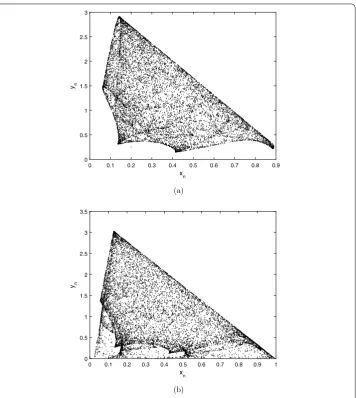
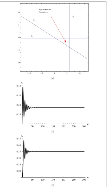
Hereafter we will provide the numerical simulation in order to verify the theoret-ical results obtained in Sect. 4.2 by fixing α2 = 1.53 and varying 1.5 ≤ α1 ≤ 18.5. Fixing α2 = 1.53, then from the non-hyperbolic condition (iii) of Lemma 5 one gets

α1= 3.1224489795918364. From a theoretical point of view the unique positive

equilib-rium point (0.6535947712418301, 0.08163300653594788) of (4) is stable if α1 < 3.1224489795918364; bifurcation occurs if α1 = 3.1224489795918364, and there is a period-doubling bifurcation ifα1> 3.1224489795918364.

Figure 2Phase portraits of the discrete-time model (4)

5.1 Fractal dimension

The fractal dimension which characterized the strange attractors of the discrete-time sys-tem is defined by (see [33,34])

dL=j+

j i=1κj

|κj|

Table 1 Numerical values ofχforα1> 2.33333

Value of bifurcation parameter whenα1> 2.33333 Numerical value ofχ

2.34 –0.11221718590370466 < 0

2.343 –0.17385157491789316 < 0

2.37 –0.17587912984797172 < 0

2.34567 –0.23250816667811489 < 0

2.4 –0.23591771770576037 < 0

2.467 –0.24392011825143836 < 0

2.5 –0.24740313673037914 < 0

2.59 –0.25764617193199524 < 0

3.1 –0.3335331833515125 < 0

3.22 –0.35545528698159623 < 0

where κ1,κ2, . . . ,κn are Lyapunov exponents and j is the largest integer such that

j

i=1κj≥0 and

j+1

i=1κj< 0. For our under consideration discrete-time model (4), the

fractal dimension takes the following form:

dL= 1 +

κ1

|κ2|

, κ1> 0 >κ2. (25)

If α2 = 1.53 then after some manipulation two Lyapunov exponents are κ1 = 1.3153221370247266 (resp. κ1 = 1.2928270741698256) andκ2 = –0.3806816141489094 (resp.κ2= –0.40393818528093656) forα1= 1.63 (resp.α1= 1.7). So the fractal dimension for the discrete-time model (4) is

dL= 1 +

1.3153221370247266 0.3806816141489094

= 4.455176420761466 forα1= 1.63,

dL= 1 +

1.2928270741698256 0.40393818528093656

= 4.200556721991193 forα1= 1.7.

(26)

The strange attractors for the above fixed parametric values are also plotted and presented in Figs.6(a)–6(b), which illustrate that the discrete model (4) has a complex dynamical behavior as the parameterα1increases.

6 Chaos control

In this section, we will study the chaos control by applying the state feedback control method [35,36]. By adding a feedback control law as the control forceunto the

discrete-time model (4), the controlled model (4) takes the following form:

Figure 5Phase portraits for values ofα1corresponding to Figs.3(a)–3(b)

matrixJcof the controlled system (27) is

Jc

x∗,y∗ =

a11–k1 a12–k2

a21 a22

, (28)

wherea11=α2α–2α1,a12= –

1

α2,a21=α1α2–α1–α2,a22= 1. The characteristic equation of

Jc(x∗,y∗) about (x∗,y∗) is

κ2–trJc

x∗,y∗ κ+detJc

Figure 6Strange attractor of the discrete-time model (4) forα1= 1.63 (resp.α1= 1.7) with (0.2, 0.25)

where

trJc

x∗,y∗ =a11+a22–k1,

detJc

x∗,y∗ =a22(a11–k1) –a21(a12–k2).

⎫ ⎬

⎭ (30)

Letκ1andκ2be the roots of (29) then

κ1+κ2=a11+a22–k1, (31)

κ1κ2=a22(a11–k1) –a21(a12–k2). (32)

The solutions of the equationsκ1=±1 andκ1κ2= 1 determine the lines of marginal sta-bility. These conditions confirm that|κ1,2|< 1. Suppose thatκ1κ2= 1, then from (32) one gets

l1:

α2–α1

α2

–k1+ (α1α2–α1–α2)

1

α2

+ 1

Now assuming thatκ1= 1 then from (31) and (32) one gets

In order to check how the implementation of feedback control method works and how to control chaos at an unstable state, we have performed numerical simulations. Fig-ures7(b)–7(c) show that about the unique positive equilibrium the chaotic trajectories are stabilized.

7 Conclusion

This work deals with the study of local dynamics, bifurcations and chaos control of a discrete-time predator–prey model (4) inR2

+. It is proved that the model has the bound-ary equilibriaO(0, 0),A(α1–1

have investigated local stability along their topological types about O(0, 0), A(α1–1

α1 , 0),

B(_α1

2,

α1α2–α1–α2

α2 ) by imposing the method of linearization and conclusions are presented

in Table2. We proved that aboutA(α1–1

α1 , 0) there exists a fold bifurcation when the

pa-rameters of the discrete model (4) are located in the following set:

F_A(α1–1

α2 ) the discrete-time model (4) undergoes

both a Neimark–Sacker bifurcation and a period-doubling bifurcation when the parame-ters, respectively, are located in the following sets:

N_B(1

Acknowledgements

The author thanks the main editor and referees for their valuable comments and suggestions leading to improvement of this paper. This work was supported by the Higher Education Commission (HEC) of Pakistan.

Funding

The author declares that he got no funding on any part of this research.

Competing interests

The author declares that he has no conflict of interests regarding the publication of this paper.

Authors’ contributions

The author carried out the proof of the main results and approved the final manuscript.

Publisher’s Note

Springer Nature remains neutral with regard to jurisdictional claims in published maps and institutional affiliations.

Received: 3 September 2018 Accepted: 28 January 2019

References

1. Volterra, V.: Leçons sur la Théorie Mathématique de la Lutte pour la Vie. Gauthier-Villars, Paris (1931) 2. Martelli, M.: Discrete Dynamical Systems and Chaos. Longman, New York (1992)

3. Landa, P.S.: Self oscillatory models of some natural and technical processes. In: Kreuzer, E., Schmidt, G. (eds.) Mathematical Research, vol. 72, p. 23

4. Freedman, H.I.: A model of predator–prey dynamics as modified by the action of a parasite. Math. Biosci.99, 143–155 (1990)

5. May, R.M.: Stability and Complexity in Model Ecosystems. Princeton University Press, Princeton (2001) 6. Volterra, V.: Fluctuations in the abundance of a species considered mathematically. Nature118, 558–560 (1926) 7. Alebraheem, J., Hasan, Y.A.: Dynamics of a two predator-one prey system. Comput. Appl. Math.33, 67–780 (2014) 8. Sinha, S., Misra, O., Dhar, J.: Modelling a predator–prey system with infected prey in polluted environment. Appl.

Math. Model.34(7), 1861–1872 (2010)

9. Chen, Y., Changming, S.: Stability and Hopf bifurcation analysis in a prey–predator system with stage-structure for prey and time delay. Chaos Solitons Fractals38(4), 1104–1114 (2008)

10. Gakkhar, S., Singh, A.: Complex dynamics in a prey–predator system with multiple delays. Commun. Nonlinear Sci. Numer. Simul.17(2), 914–929 (2012)

11. Yan, J., Li, C., Chen, X., Ren, L.: Dynamic complexities in 2-dimensional discrete-time predator–prey systems with Allee effect in the prey. Discrete Dyn. Nat. Soc.2016, Article ID 4275372 (2016)

12. Zhao, J., Yan, Y.: Stability and bifurcation analysis of a discrete predator–prey system with modified Holling–Tanner functional response. Adv. Differ. Equ.2018, 402 (2018)

13. Fang, Q., Li, X.: Complex dynamics of a discrete predator–prey system with a strong Allee effect on the prey and a ratio-dependent functional response. Adv. Differ. Equ.2018, 320 (2018)

14. Kangalgi, F., Kartal, S.: Stability and bifurcation analysis in a host–parasitoid model with Hassell growth function. Adv. Differ. Equ.2018, 240 (2018)

15. Li, L., Shen, J.: Bifurcations and dynamics of a predator–prey model with double Allee effects and time delays. Int. J. Bifurc. Chaos28(11), 1–14 (2018)

16. Zhao, M., Li, C., Wang, J.: Complex dynamic behaviors of a discrete-time predator–prey system. J. Appl. Anal. Comput. 7(2), 478–500 (2017)

17. Cheng, L., Cao, H.: Bifurcation analysis of a discrete-time ratio-dependent predator–prey model with Allee effect. Commun. Nonlinear Sci. Numer. Simul.38, 288–302 (2016)

18. Liu, W., Cai, D., Shi, J.: Dynamic behaviors of a discrete-time predator–prey bioeconomic system. Adv. Differ. Equ. 2018, 133 (2018)

19. Liu, X., Chu, Y., Liu, Y.: Bifurcation and chaos in a host–parasitoid model with a lower bound for the host. Adv. Differ. Equ.2018, 31 (2018)

20. Sohel Rana, S.M.: Chaotic dynamics and control of discrete ratio-dependent predator–prey system. Discrete Dyn. Nat. Soc.2017, Article ID 4537450 (2017)

21. Zhao, M., Du, Y.: Stability of a discrete-time predator–prey system with Allee effect. Nonlinear Analy. Diff. Equ.4(5), 225–233 (2016)

22. Liu, X., Xiao, D.: Complex dynamic behaviors of a discrete-time predator–prey system. Chaos Solitons Fractals32(1), 80–94 (2007)

23. Khan, A.Q., Ma, J., Xiao, D.: Bifurcations of a two-dimensional discrete time plant-herbivore system. Commun. Nonlinear Sci. Numer. Simul.39, 185–198 (2016)

24. Khan, A.Q., Ma, J., Xiao, D.: Global dynamics and bifurcation analysis of a host–parasitoid model with strong Allee effect. J. Biol. Dyn.11(1), 121–146 (2017)

25. Khan, A.Q.: Stability and Neimark–Sacker bifurcation of a ratio-dependence predator–prey model. Math. Methods Appl. Sci.40(11), 3833–4232 (2017)

26. Hu, Z., Teng, Z., Zhang, L.: Stability and bifurcation analysis of a discrete predator–prey model with non-monotonic functional response. Nonlinear Anal., Real World Appl.12(4), 2356–2377 (2011)

27. Jing, Z., Yang, J.: Bifurcation and chaos in discrete-time predator–prey system. Chaos Solitons Fractals27(1), 259–277 (2006)

29. Sen, M., Banerjee, M., Morozov, A.: Bifurcation analysis of a ratio-dependent prey–predator model with the Allee effect. Ecol. Complex.11, 12–27 (2012)

30. Guckenheimer, J., Holmes, P.: Nonlinear Oscillations, Dynamical Systems and Bifurcation of Vector Fields. Springer, New York (1983)

31. Kuznetsov, Y.A.: Elements of Applied Bifurcation Theory, 3rd edn. Springer, New York (2004)

32. Khan, A.Q.: Supercritical Neimark–Sacker bifurcation of a discrete-time Nicholson–Bailey model. Math. Methods Appl. Sci.41(12), 4841–4852 (2018)

33. Cartwright, J.H.E.: Nonlinear stiffness Lyapunov exponents and attractor dimension. Phys. Lett. A264, 298–304 (1999) 34. Kaplan, J.L., Yorke, J.A.: Preturbulence: a regime observed in a fluid flow model of Lorenz. Commun. Math. Phys.67(2),

93–108 (1979)

35. Elaydi, S.N.: An Introduction to Difference Equations. Springer, New York (1996)