R E S E A R C H
Open Access
Automatic ARIMA modeling-based data
aggregation scheme in wireless sensor networks
Guorui Li
1*and Ying Wang
2Abstract
Data aggregation is a very important method to conserve energy by eliminating the inherent redundancy of raw data in wireless sensor networks (WSNs). In this article, we developed an automatic auto regressive-integrated moving averagemodeling-based data aggregation scheme in WSNs. The main idea behind this scheme is to decrease the number of transmitted data values between sensor nodes and aggregators by utilizing time series prediction model. The proposed scheme can effectively save the precious battery energy of wireless sensor nodes while keeping the predicted data values of aggregators within application-defined error threshold. We show through experiments with real data that the predicted data values of our proposed scheme fit the real sensed data values very well and fewer messages are transmitted between sensor nodes and aggregators than the native data aggregation scheme. Furthermore, the characteristics of the proposed data aggregation scheme are also discussed in this article.
Keywords:Wireless sensor networks, Data aggregation, Time series analysis, ARIMA model, Pediction
1. Introduction
Wireless sensor networks(WSNs) are made up of a mass of spatially distributed autonomous sensor nodes, to jointly monitor physical or environmental conditions, such as temperature, humidity, vibration, pressure, sound, motion, or pollutants [1]. These sensors could be scattered randomly in harsh environments such as bat-tlefields or deterministically placed at specified locations to collect information from the environment. The typical application fields of WSNs include industrial process control, security and surveillance, traffic control, home automation, environmental sensing, structural health monitoring, etc. [2].
In WSNs, the communication cost of sensor node is often several orders of magnitude higher than that of computation. For instance, the transmission and reception energy costs for one bit of MICAz node [3] and TelosB node [4] are 600, 670, and 720, 810 nJ, respectively. However, the computation energy costs for 1 bit of them are only 3.5 and 1.2 nJ, respectively [5]. Therefore, data aggregation scheme is often adopted as an effective way to
save the precious battery energy of wireless sensor nodes by eliminating the inherent redundancy in the raw data and avoiding unnecessary data transmission. Moreover, data aggregation scheme is also useful to extract application-specified general information from the raw data which are collected from the sensor nodes [6]. Hence, it is critical for WSNs to support data aggregation schemes.
There have been plenty of researches in the recent past on data aggregation schemes in WSNs. Typically, the whole sensor network is partitioned into hierarchical structure which consists of sink node, aggregators, and ordinary sensors. The aggregator utilizes specific functions, such as mean, min, or max, to aggregate incoming readings, and only the aggregated results are forwarded to the sink. Therefore, communication overhead can be reduced and packet collision can be avoided by decreasing the amount of transmitted messages. A comprehensive survey on data aggregation schemes of WSN was presented in [7]. And we will briefly review some representative data aggregation schemes in Section 2.
In this article, we proposed an automatic auto regressive-integrated moving average (ARIMA)modeling-based data aggregation scheme which utilizes time series model to pre-dict the data of next several periods at both ordinary sensor nodes and aggregators based on the same amount of recent * Correspondence:[email protected]
1
School of Computer and Communication Engineering, Northeastern University at Qinhuangdao, Qinhuangdao, China
Full list of author information is available at the end of the article
data values. The sensor node will build an appropriate time series model to predict the future data based on recently sensed data values and transmit the parameters of the model to the aggregator automatically. When the predic-tion error between the sensed value and predicted value is within the application-specified error threshold, sensor node will not transmit the sensed value to the aggregator. In this case, the aggregator will regard the predicted value as the sensed value in current data collection period. When the prediction error is beyond the application-specified error range, the sensor node will rebuild the time series model and transmit the sensed value with the new model to the aggregator in order to replace the incorrect predicted value and unsuited prediction model. We show through experiments that the predicted values of our proposed scheme fit the real sensed values very well and fewer messages are required to transmit between sensor nodes and aggregators.
The remainder of this article is organized as follows. In Section 2, we review some related works. In Section 3, we present our automatic ARIMA modeling-based data aggregation scheme. In Section 4, we describe our experiment settings and evaluation results. Finally, we conclude this article and present future directions in the Section 5.
2. Related works
There have been extensive researches in the field of data aggregation scheme in WSNs. According to the underlying route structure, the proposed data aggregation schemes can be categorized into four classes: tree-based data aggregation scheme, cluster-based data aggregation scheme, multi-path data aggregation scheme, and hybrid data aggregation scheme [8].
In tree-based data aggregation scheme, a spanning tree rooted at the sink is constructed and data aggregation operations proceed level-by-level from its leaves to its root. However, the cost of maintaining such a dynamic hierarchical tree structure is very high. In cluster-based data aggregation scheme, sensor nodes are divided into clusters and some special nodes, referred to as cluster heads, are selected to aggregate data locally and forward the result to the sink. In order to balance the energy cost of data aggregation, cluster head is rotated within the cluster. In multi-path data aggregation scheme, data are sent over multiple paths and aggregation is performed over these paths as packets move towards the sink level-by-level. In this kind of scheme, higher robustness is achieved by inducing extra overhead. Hybrid data aggregation scheme tries to overcome the problems of both the tree- and multi-path-based structures by combining the best features of both schemes. Hence, the whole network is organized into regions implementing one of the above two schemes.
And the main difficulty is how to connect regions running different aggregation schemes.
However, none of the above data aggregation schemes have considered the problem of decreasing the number of transmitted data values between ordinary sensors and aggregator. They take for granted that sensor nodes periodically report sensed data values to the aggregator. However, the energy cost of data transmission and reception between them is not trivial. That is the focus and motivation of this article.
3. Automatic ARIMA modeling-based data aggregation scheme
Since the data generated by sensor nodes during continuously monitoring periods usually are of high temporal correlation, it indicates that there are redundant data in the successive data sequence, which causes unnecessary data transmission and energy consumption. In this article, we only focus on data transmission reduction and corresponding energy saving between sensor nodes and aggregators. Furthermore, we assume that a reliable message retransmission mechanism is adopted in the under-lying MAC layer to guarantee the ARIMA model parameters and sensed data values could be delivered to the aggregator successfully even after collusion happens.
The automatic ARIMA modeling-based data aggrega-tion scheme utilizes ARIMA model to predict the data of next several periods at both ordinary sensors and aggregators based on the same amount of recently sensed values. The ordinary sensors and aggregators work coordinately to reduce the amount of messages transmitted within the network.
3.1. The ARIMA model
Time series analysis uses historical data to develop a model for the prediction of future data values. The ARIMA model, also called Box–Jenkins model, is a widely used prediction model for univariate time series [19]. An ARIMA process can be divided into three components: auto-regressive (AR), moving-average (MA), and one-step differencing. The AR component estimates the current sample as a linear-weighted sum of previous samples; the MA compo-nent captures relationship between prediction errors; and the one-step differencing component captures relationship between adjacent samples. In ARIMA, the AR component captures the temporal correlation in the time series by modeling a future value as a function of a number of past values. The MA com-ponent is modeled as a zero-mean, uncorrelated Gaussian random variable (also referred to as white noise) [20].
The ARIMA(p,d,q) model of time series {x1,x2,…} is
defined as
Φpð ÞBΔdxt¼Θqð ÞB εt ð1Þ
where B is the backward shift operator, Δ is the back-ward difference, d is the order of differencing, and Φp
andΘqare polynomials of orderpandq, respectively.
Bxy¼xy−1 ð2Þ
The parameters Φand Θare chosen so that the zeros of both polynomials lie outside the unit circle in order to avoid generating unbounded processes.
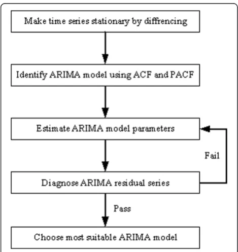
The construction steps of ARIMA model are shown in Figure 1. It includes the following five steps [21].
Step 1: Make time series stationary by differencing
The noise series being analyzed must be stationary. When the variance of the noise series is non-stationary, the data must be transformed by differencing the original data to make the series stationary. If the series exhibits a trend over time or seasonality, or if some other non-stationary pattern exists, the series should be differenced repeatedly until the time series becomes stationary.
Step 2: Identify the model using ACF and PACF.
Candidate ARIMA models are identified once the time series becomes stationary. After obtaining the autocor-relation function (ACF) and partial autocorautocor-relation func-tion (PACF), multiple ARIMA models that closely fit the data can be identified. The k-order autocorrelation coef-ficient of time series {x1,x2,…} is defined as
The k-order partial autocorrelation coefficient of time series {x1,x2,…} is defined as follows:
Step 3: Estimate ARIMA model parameters.
After identifying a possible ARIMA model, we analyze the time series and estimate the model parameters. If the PACF of the differenced series displays a sharp cutoff and the lag-1 autocorrelation is positive, then consider adding one or more AR terms to the model. The lag beyond which the PACF cuts off is the indicated number of AR terms. If the ACF of the differenced series displays a sharp cutoff and the lag-1 autocorrelation is negative, then consider adding an MA term to the model. The lag be-yond which the ACF cuts off is the indicated number of MA terms.
Step 4: Diagnose ARIMA residual series.
This step employs a white noise test to check whether the residual series from the model contains additional
information that might be of use to a more complex model. In this case, the analysis must be continued by repeating Steps 3 and 4 until an appropriate ARIMA model is found which passes the white noise test.
Step 5: Choose the most suitable ARIMA model.
An ARIMA model with the smallest Akaike Informa-tion Criterion (AIC) indicator or Bayesian InformaInforma-tion Criterion (BIC) indicator is selected as the most suitable ARIMA model for analysis.
The AIC indicator and BIC indicators are calculated as follows:
AIC¼−2l=Tþ2k=T ð9Þ
BIC¼−2l=TþðklogTÞ=T ð10Þ
In Equations (9) and (10), l is the log likelihood,T is the number of observations, k is the number of right-hand side regressors, and^ε′^ε in Equation (11) is the sum
The power of an ARIMA model resides in that it can incorporate all the AR term, the integrated term, and the moving average term together to model time series with a wide variety of features such as trend by simply adjusting the parameters of each term.
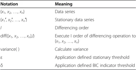
Table 1 Notations
ε Application defined stationary threshold
3.2. Data aggregation scheme
The ordinary sensor node runs automatic ARIMA modeling algorithm to build ARIMA prediction model automatically. The notations used in the algorithm are described in Table 1.
The automatic ARIMA modeling algorithm works as follows:
In order to build ARIMA prediction model, sensor node needs to collect recently sensed data series {x1,
x2, …, xn}. If {x1, x2, …, xn} is not stationary, we
should make the differencing adjustment to data series until the difference between successive vari-ances is smaller than the application-defined station-ary threshold ε. Then, we fit ARIMA prediction model according to the differenced data series {x1′,
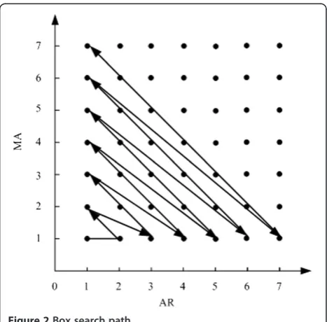
x2′, …, xn′} using least square method. The iteration
of ARIMA model fitting process follows the Box search path, which is shown in Figure 2. It can find an appropriate fitting model using a relatively small number of search times [22]. When the BIC indicator of an ARIMA model is smaller than the application-defined BIC threshold δ and the corresponding Ljung Box white noise test of fit residual passes, the iter-ation of ARIMA model fitting process will stop. In other words, an appropriate ARIMA prediction model has been built. Here, we choose BIC indicator over AIC indicator for the reason that BIC indicator is more consistent and penalizes free parameters more
The automatic ARIMA modeling-based data aggregation scheme works as follows:
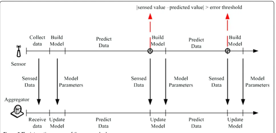
First of all, the ordinary sensor node runs automatic ARIMA modeling algorithm to build an appropriate ARIMA prediction model. It then sends the ARIMA model parameters to aggregator. After that, it calculates the predicted value according to ARIMA model and compares the sensed value with the predicted value. If the difference between them is less than the predefined error threshold, the sensor node will store the predicted value into historical data queue. Otherwise, it will store the sensed value into historical data queue and send the sensed value to aggregator at the same time. When the predicted value is beyond the fault tolerant range of the sensed value, the AIRMA model will be rebuilt and corre-sponding ARIMA model parameters of aggregator will be refreshed again.
in the underlying MAC layer to guarantee the sensed value could be delivered to aggregator even after collusion happens.
The detailed interactive process of automatic ARIMA modeling-based data aggregation scheme is shown in Figure 3. The ordinary sensor node and aggregator work coordinately to decrease the number of transmitted messages between them. The shaded circles in the figure indicate that the difference between sensed value and predicted value is beyond the fault tolerant range. In other words, the prediction model should be rebuilt and updated.
4. Evaluations
In this section, we evaluate and compare the performance of automatic ARIMA modeling-based data aggregation scheme with native data aggregation scheme without data prediction. We use the real-sensed data collected from TAO (Tropical Atmosphere Ocean)
project to demonstrate the performance of our proposed scheme. The TAO project provides real-time collection of high-quality oceanographic and surface meteorological data for monitoring, forecasting, and understanding of climate swings associated with El Niño and La Nina since 1982 [23]. The collected data include sea surface temperature, sea level pressure, salinity, relative humidity and density, etc., along with timestamp information collected once every 10 min. We will only use the sea surface temperature data to evaluate our scheme. The other collected measurement will produce the similar results. Figure 4 shows a detailed deployment of nearly 70 buoys of TAO project.
4.1. Performance comparison
In automatic ARIMA modeling-based data aggregation scheme, ordinary sensor node will transmit the sensed data value to the aggregator only when the prediction error between sensed value and predicted value is Figure 3The interactive process of the proposed scheme.
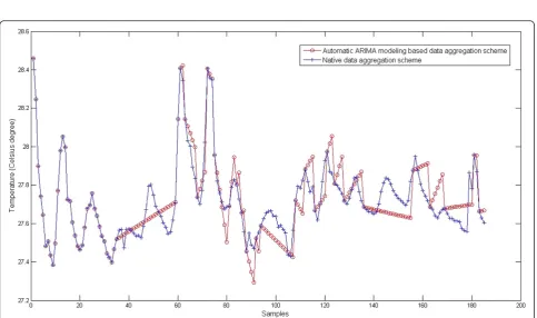
Figure 5Data comparison of two schemes when the error threshold is set to 0.1°C.
beyond the application-specified error threshold. In na-tive data aggregation scheme without data prediction, ordinary sensor node will transmit all the sensed data values to the aggregator. We will refer to it as native data aggregation scheme in the rest of this article. It is noteworthy that we only consider the problem of data transmission between ordinary sensor node and data aggregator. Both schemes can be combined with other data aggregation schemes which deal with data ag-gregation between aggregator and sink.
Figures 5 and 6 show the comparison of sensed data values of native data aggregation scheme and predicted data values of automatic ARIMA modeling-based data aggregation scheme with different predefined error threshold, 0.1 and 0.2°C, respectively. The source data values which are used to build ARIMA prediction model
were collected from the buoy deployed at 8° north latitude 155° west longitude. We can conclude that the predicted values of our scheme fit the sensed values very well. And the less the predefined error threshold, the better the predicted values fit the sensed values. On the contrary, more ARIMA prediction models should be rebuilt to satisfy the error threshold condition. We will discuss this property further in the next section.
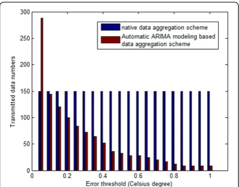
Figure 7 shows the comparison of transmitted data numbers of both data aggregation schemes when the number of predicted values is set to 150. In native data aggregation scheme, all the sensed data values should be sent to the aggregator. In automatic ARIMA modeling-based data aggregation scheme, only the sensed data values which are beyond the error tolerance range and the ARIMA model parameters should be sent to the aggregator. We can see that automatic ARIMA modeling-based data aggregation scheme transmits much less number of messages than native data aggregation scheme for most of the times. Consequently, precious battery energy of wireless sensor nodes is saved and much longer network lifetime is maintained. Only when the error threshold is set too small, many ARIMA prediction models are unfitted and should be rebuilt. Therefore, the transmission of corresponding ARIMA model parameters outnumbers the transmission of sensed data values.
4.2. Performance evaluation
In this section, we evaluate the performance of automatic ARIMA modeling-based data aggregation scheme.
Figure 8 shows the ARIMA model rebuild times of our proposed scheme at different error threshold when the number of predicted values is set to 150 and histor-ical data size is set to 35. And corresponding average prediction number of ARIMA model is shown in Figure 7Comparison of transmitted data numbers.
Figure 9. We can see that the ARIMA model rebuild times decreases with the increase of error threshold. And average prediction number of ARIMA model increases with the increase of error threshold. The reason behind this pattern lies in the fact that larger error threshold implies wider prediction range an ARIMA model can achieve.
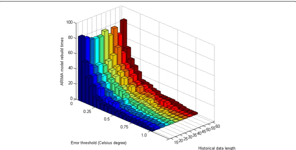
Figure 10 demonstrates the influence of error thresh-old and historical data length on ARIMA model rebuild times in an overall view. We can draw the conclusion that error threshold is inversely proportional to ARIMA
model rebuild times. And historical data length has no prominent influence on ARIMA model rebuild times. However, larger historical data length implies more com-putation cycles and memory usage. Hence, we should adopt large error threshold and small historical data length in order to increase the network lifetime of wireless sensor node.
When the predicted value is beyond the fault tolerant range of the sensed value, the ARIMA model should be rebuilt and corresponding ARIMA model parameters should be transmitted to the aggregator. Therefore, the Figure 10Multiple ARIMA model rebuild times.
cost of ARIMA model rebuild is composed of two parts, the computation cost of ARIMA model and the transmis-sion cost of ARIMA model parameters. The computation of ARIMA model is executed in the ordinary sensor node with the cost of a small number of search times [20]. It is well known that the communication cost is often several orders of magnitude higher than that of computation. Hence, the computation cost of ARIMA model is relatively low. After that, several bytes of ARIMA model parameters are transmitted from ordinary sensor to the aggregator. Compare with the general data and control message transmission within the network, the cost of model parameters transmission can be negligible.
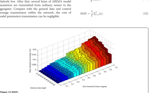
To evaluate the prediction accuracy of automatic ARIMA modeling-based data aggregation scheme, we measure the prediction error and investigate the following three prediction accuracy indicators:mean squared error (MSE), mean absolute error (MAE), and mean absolute percentage error (MAPE), respectively.
MSE¼ 1 T∑
T
t¼1e2t ð12Þ
MAE¼ 1 T∑
T
t¼1j jet ð13Þ
Figure 12MAE.
MAPE¼ 1
In Equations (12), (13), and (14), prediction erroret=
yt–pt, whereytis sensed value andptis predicted value.
The influence of error threshold and historical data length on MSE, MAE, and MAPE are shown in Figures 11, 12, and 13, respectively. We can see from the figures that pre-diction accuracy decreases with the increase of the predefined error threshold and increases with the increase of historical data length. The reason behind this property lies in the fact that larger error threshold implies wider error tolerance range, which will result in lower prediction accuracy. Larger historical data length implies more precise prediction model, which will result in higher prediction accuracy. Hence, we should adopt small error threshold and large historical data length in order to improve the prediction accuracy of our proposed scheme.
5. Conclusion
We have introduced automatic ARIMA modeling-based data aggregation scheme in this article. Our motivation is to suppress the unnecessary transmitted data values be-tween ordinary sensors and aggregator by data prediction. We first presented the ARIMA prediction model and then described how the ARIMA prediction model could be built and applied in data aggregation scheme to decrease the number of transmitted messages within the network. Our simulation and analysis indicate that the predicted values of our proposed scheme fit the real sensed values very well and fewer messages are required to transmit between sensor node and aggregator. The relationships between scheme performance and scheme parameters are also discussed in this article.
As a future work, we would like to improve our proposed data aggregation scheme by utilizing spatial and temporal data correlation characteristics to-gether. Furthermore, we would like to implement automatic ARIMA modeling-based data aggregation scheme into a WSN testbed and evaluate its per-formance too.
Competing interests
The authors declare that they have no competing interests.
Acknowledgments
We would like to thank the anonymous reviewers for their constructive comments and suggestions on improving the presentation of this study. We also would like to thank the TAO Project Office of NOAA/PMEL for allowing us to use the TAO data. The study was supported by the Fundamental Research Funds for the Central Universities of China (Program no. N100323001 and N120423005), the Natural Science Foundation of Hebei Province, China (Grant no. F2012501014), the Scientific Research Foundation of the Higher Education Institutions of Hebei Province, China (Grant no. Z2010215), the Research Fund for the Doctoral Program of Higher Education
of China (Grant no. 20120042120009), and the Science and Technology Research and Development Project of Qinhuangdao (Grant no. 2012021A029).
Author details 1
School of Computer and Communication Engineering, Northeastern University at Qinhuangdao, Qinhuangdao, China.2Department of Information Engineering, Qinhuangdao Institute of Technology, Qinhuangdao, China.
Received: 12 November 2011 Accepted: 27 February 2013 Published: 25 March 2013
References
1. G Li, J He, Y Fu, Group-based intrusion detection system in wireless sensor networks. Comput. Commun.31(18), 4324–4332 (2008)
2. J Yick, B Mukherjee, D Ghosal, Wireless sensor network survey. Comput. Netw.52(12), 2292–2330 (2008)
3. Micaz(US Memsic, Andover, 2011). http://www.memsic.com. Accessed 11 November 2011
4. TelosB(US Memsic, Andover, 2011). http://www.memsic.com. Accessed 11 November 2011
5. G Meulenaer, F Gosset, F Standaert, O Pereira, On the energy cost of communication and cryptography in wireless sensor networks, in
Proceedings of IEEE International Conference on Wireless and Mobile ComputingAvignon, France, 2008), pp. 580–585
6. S Lee, S Kim, D Ko, S Kim, S An, Prediction based mobile data aggregation in wireless sensor network, inProceedings of 4th International Conference on Advances in Grid and Pervasive ComputingGeneva, Switzerland, 2009), pp. 328–339
7. R Rajagopalan, P Varshney, Data-aggregation techniques in sensor networks: a survey. IEEE Commun. Surv. Tutor.8(4), 48–63 (2006)
8. E Fasolo, M Rossi, J Widmer, M Zorzi, In-network aggregation techniques for wireless sensor networks: a survey. IEEE Wirel. Commun.14(2), 70–87 (2007) 9. W Heinzelman, A Chandrakasan, H Balakrishnan, An application-specific
protocol architecture for wireless microsensor networks. IEEE Trans. Wirel. Commun.1(4), 660–670 (2002)
10. S Lindsey, C Raghavendra, PEGASIS: power-efficient gathering in sensor information systems, inProceedings of IEEE Aerospace Conference
Montana, USA, 2002), pp. 1125–1130
11. C Intanagonwiwat, D Estrin, R Goviindan, J Heidemann, Impact of network density on data aggregation in wireless sensor networks, inProceedings of 22nd International Conference on Distributed Computing SystemsVienna, Austria, 2002), pp. 457–458
12. W Zhang, G Cao, DCTC: dynamic convoy tree-based collaboration for target tracking in sensor networks. IEEE Trans. Wirel. Commun.3(5), 1689–1701 (2004) 13. M Ding, X Cheng, G Xue, Aggregation tree construction in sensor networks,
inProceedings of IEEE 58th Vehicular Technology ConferenceOrlando, USA, 2003), pp. 2168–2172
14. H Xu, L Huang, Y Zhang, H Huang, S Jiang, G Liu, Energy-efficient cooperative data aggregation for wireless sensor networks. J. Parallel Distrib. Comput.70(9), 953–961 (2010)
15. L Villas, A Boukerche, H Oliveira, R Araujo, A Loureiro, A spatial correlation aware algorithm to perform efficient data collection in wireless sensor networks. Ad Hoc Netw.11(3), 966–983 (2013)
16. H Yousefi, M Yeganeh, N Alinaghipour, A Movaghar, Structure-free real-time data aggregation in wireless sensor networks. Comput. Commun.
35(9), 1132–1140 (2012)
17. L Xiang, J Luo, A Vasilakos, Compressed data aggregation for energy efficient wireless sensor networks, inProceedings of 8th IEEE Conference on Sensor, Mesh and Ad Hoc Communications and NetworksSalt Lake City, USA, 2011), pp. 46–54
18. L Xiang, J Luo, C Deng, A Vasilakos, W Lin, DECA: recovering fields of physicals quantities from incomplete sensory data, inProceedings of 9th IEEE Conference on Sensor, Mesh and Ad Hoc Communications and Networks
Seoul, Korea, 2012), pp. 182–190
19. G Box, G Jenkins, G Reinsel,Time Series Analysis: Forecasting and Control, 4th edn. (Wiley, NJ, 2008), pp. 47–92
21. G Li, Y Wang, A prediction based data aggregation scheme in wireless sensor networks. Adv. Mater. Res.268–270, 517–522 (2011)
22. S Yang, Y Wu, J Xuan,Time Series Analysis in Engineering Application, 2nd edn. (HUST Press, Wuhan, 2007), pp. 265–269
23. TAO project(US NOAA, Seattle, 2011). http://www.pmel.noaa.gov/tao. Accessed 11 November 2011
doi:10.1186/1687-1499-2013-85
Cite this article as:Li and Wang:Automatic ARIMA modeling-based
data aggregation scheme in wireless sensor networks.EURASIP Journal on Wireless Communications and Networking20132013:85.
Submit your manuscript to a
journal and benefi t from:
7Convenient online submission
7Rigorous peer review
7Immediate publication on acceptance
7Open access: articles freely available online
7High visibility within the fi eld
7Retaining the copyright to your article