Lists in a Lighthouse

University of South Carolina

Scholar Commons

Theses and Dissertations

2015

Adaptivity For Meshfree Point Collocation

Methods In Linear Elastic Solid Mechanics

University of South Carolina

Follow this and additional works at:https://scholarcommons.sc.edu/etd

Part of theCivil Engineering Commons

This Open Access Thesis is brought to you by Scholar Commons. It has been accepted for inclusion in Theses and Dissertations by an authorized administrator of Scholar Commons. For more information, please [email protected].

Recommended Citation

ADAPTIVITY FOR MESHFREE POINT COLLOCATION METHODS IN LINEAR ELASTIC SOLID MECHANICS

by

Joshua Wayne Derrick Bachelor of Science in Engineering University of South Carolina, 2013

Submitted in Partial Fulfillment of the Requirements For the Degree of Master of Science in

Civil Engineering

College of Engineering and Computing University of South Carolina

2015 Accepted by:

Robert L. Mullen, Director of Thesis Juan Caicedo, Reader

Joseph Flora, Reader Shamia Hoque, Reader

A

A

This study presents the behavior of local node adaptivity for point collocation meshfree numerical methods and its application to linear elastic solid mechanics. A bisection approach to meshfree adaptivity will be presented with numerical examples showing that convergence is achieved. A threshold value is required from the user and this value is an acceptable change in gradient for the problem. If the change in gradient between 2 nodes exceed this limit, a node is added at the mid-point between the two nodes. This process applies to all nodes in the model. Once the refinement is complete, the model is processed again and this procedure is repeated until the program reaches a limit of iterations or the acceptable error is achieved.

T

C

ACKNOWLEDGEMENTS ... iii

ABSTRACT ... iv

LIST OF TABLES ... vi

LIST OF FIGURES ... vii

CHAPTER 1INTRODUCTION ...1

CHAPTER 2:LITERATURE REVIEW ...8

CHAPTER 3:FORMULATION OF THE PARTICLE DIFFERENCE METHOD...11

CHAPTER 4:COMPUTER IMPLEMENTATION ...19

CHAPTER 5:NUMERICAL EXAMPLES ...22

CHAPTER 6:DISCUSSION ON THE LOCAL INFLUENCE PARAMETER ...35

CHAPTER 7:SUMMARY AND CONCLUSIONS ...37

L

T

L

F

Figure 3.1 PDA Weight Function ...4

Figure 5.1 2D Cantilever Beam Problem ...10

Figure 5.2 2D Cantilever Beam Model ...23

Figure 5.3 Global Refinement for Cantilever Beam ...25

Figure 5.4 Relative Error of Cantilever Beam ...30

Figure 5.5 2D Plate with Hole ...34

Figure 5.6 2D Plate with Hole Partition...4

Figure 5.7 2D Plate with Hole Model ...10

Figure 5.8 Global Refinement for Plate with Hole ...23

Figure 5.9 Relative Error of Plate with Hole ...25

Figure 5.10 Local Refinement of Cantilever Beam ...30

Figure 5.11 Relative Error of Cantilever Beam with Adaptivity ...34

Figure 5.12 Local Refinement of Plate with Hole ...23

Figure 5.13 Relative Error of Plate with Hole with Adaptivity ...25

CHAPTER

1

I

Computer simulations are powerful tools for practicing and research engineers due to the increasing power in computer technology and ability to simulate full scale engineered systems without the need to run expensive and potentially dangerous laboratory experiments. Computer simulation software is driven primarily by the numerical methods developed to approximate complex equations that do not have an obtainable analytical solution. These complex equations are often Partial Differential Equations (PDE) that describe the physics of a system, but cannot be easily solved analytically.

Meshed Methods and Meshfree Methods.

Numerical methods used to approximate the solution for PDE’s can be divided into two categories: meshed methods and meshfree methods.

Meshed methods are numerical methods that require a mesh for the purposes of approximating the integral form of a PDE. Mesh is a geometric representation of a model constructed from an arrangement of elements and nodes where elements are lines (1D models), triangles, quadrilaterals (2D models), tetrahedrons, pentahedrons and hexahedrons (3D models) and nodes are the vertices of each on an element. Typically, elements have assigned interpolation schemes to convert the nodal approximations to a functional representation over the domain of that element. This allows the model to have a continuous function to determine the solution values at any point in the model based on the nodal solutions only. One purpose of having mesh is to use the nodal solutions and element interpolants to obtain the functions over that element. When the union of all elements form the problem domain, a function can be constructed for the entire model allowing access to the solution values at any point in that model.

approximation scheme in which a weighted function is expanded about each node to form a derivative approximation based on the relative location of the surrounding nodes. The detail of the LSM used in this research will be expanded more in chapter 3.

Using meshed based numerical methods is sometimes cumbersome due to the complexity of the models’ geometry. Mesh generation can be difficult for models with complex geometries and ill-conditioned solutions can result from certain mesh constructions, for example when the mesh is highly distorted. The interest for meshfree technology is also motivated by the absence of mesh and eliminating the need for complex computational geometry programs. Computational geometry programs can be very time consuming and computationally expensive depending on the fineness of the model and the degree of accuracy prescribed. In meshed methods, nodal data and element data is required for the operations, where in meshfree methods, only nodal data is needed for the approximation schemes.

Numerical Methods in Solid Mechanics.

In the field of solid mechanics, numerical methods are typically used for stress analysis, meaning, as forces are applied to a non-rigid body, the body deforms and internal energy is developed which leads to the development of stress in that body. Some of the most common methods are the Finite Difference Method (FDM), Boundary Element Method (BEM) and Finite Element Method (FEM).

dependent, in other words, the solution of a node depends on the solution of the surrounding nodes. The grid needed for most FDM’s can introduce more difficulties compared to general mesh based methods, as the grid is needed to be well structured. The FDM can be a less desirable choice for modeling due to the node arrangement restriction making it difficult to model problems with curved boundaries or inclusions, also, it is not well suited for modeling discontinuities.

The Boundary Element Method (BEM) is a meshed numerical method that discretizes the boundary of a problem into elements and nodes and uses a boundary integral formulation to approximate the weak form. The BEM uses polynomial interpolants to approximate the solutions in the domain between known solutions on the boundary. The BEM requires that a fundamental solution be known for the method to work, however, the fundamental solution are known for only a limited number of linear PDE’s.

be problematic to work with when modeling complex problems due to the computational requirements needed to process the data such as complex 3D geometries, multi-physics modeling, discontinuities, etc.

The Element-Free Galerkin Method (EFGM) [1] is a meshfree numerical method that uses nodes only and incorporates the Moving Least Squares Method (MLSM) to approximate the derivatives of the weight functions for the weak form of a differential equation. The EFGM does, however, use a background mesh to generate a nodal discretization. Once the nodal solutions are known, Gauss Integration of each cell is used to compute the integral form.

Developments in Meshfree Methods.

Meshfree numerical methods have become a more popular choice for modeling since they do not require the computational power and resources like meshed methods. Meshfree methods are very popular in studies regarding fracture mechanics and crack propagation because the mesh refinement process is not required for approximations as cracks propagate through a body. Several methods have been introduced into modeling fracture such as that in [1, 2, 3] where the meshfree method is used with enriched weight functions for modeling fatigue crack growth. Another meshfree method was presented for modeling elastic cracks in [2] where a point collocation scheme based on diffuse derivatives was presented.

Concept of Adaptivity.

with two difference approaches: h-adaptivity and p-adaptivity. H-adaptivity is the idea of using smaller elements in regions with a high gradient in the solution, where p-adaptivity is the process of using a higher order interpolant for smoothing out a solution where the current interpolant is not capturing all of the effects of the nodal solution. Another approach to adaptivity is L-adaptivity in which the discretizations are moved based on the solution. In the FEM, L-adaptivity is moving existing nodes closer to the regions with high gradients so that refinement is completed without the need to add elements. In meshfree methods, h-adaptivity is the most commonly form of adaption practiced. Meshfree adaptivity is a popular practice due to the simplicity of refinement for meshfree methods. To adapt a model that only contains points simply means adding more points in strategically computed locations.

Summary of Study.

CHAPTER 2

L

R

The use of adaptive methods in numerical analysis is quiet extensive. Here, the focus is on adaptivity in meshfree methods. Adaptivity for meshfree numerical methods are motivated by the reduction in numerical modeling by local refinement strategies rather than defining an extremely fine model that could be extremely computationally expensive or time consuming.

Adaptivity has been implemented primarily for problems involving complex physics such as fracture mechanics or crack propagation. Belytschko and Rabczuk [4] implemented the algorithm they proposed in [5] to model arbitrary evolving cracks and large deformation by including enrichment functions to mathematically model the discontinuity in the domain.

A common approach is using a structured grid of nodes and defining cells that connect the nodes. Ling [6] proposed an adaptive method in which the model was discretized into a structured grid of nodes and square or cubic cells were defined as a background node connectivity mesh depending on the dimension of the problem. The algorithm proposed refined cells based on a cell principal value and if the cell met the refinement criteria, the cell was subdivided by quadrisection which is dividing 1 cell into 4 cells. Belytschko and Rabczuk [5] also proposed an adaptivity algorithm based on background cells in which each cell was quadrisected into 4 cells based on the energy in that cell. The difference between the work developed by Ling and Belytschko is that Ling does not use cell-wise integration to determine which regions will be adapted with more nodes where Rabczuk and Belytschko use background cells to determine the error based on the energy norm.

other words, meshfree methods are highly sensitive to node distributions and triangulated cells with centroidal adaption could add more nodes to one side of a triangular cell and result in too many nodes in a localized region.

In this study, the adaptivity is truly meshfree in the since there are no background cells or background elements for integration. The error estimator is the L2 norm of the

CHAPTER

3

F

P

D

M

In this section, the Particle Derivative Approximation (PDA) is derived as presented in [2]. This meshfree numerical method is a point collocation numerical method used to directly approximate the strong form where methods such as the EFGM is used to approximate the weak form. The PDA was constructed in the framework of the Moving Least Squares Method (MLSM) which is a numerical differentiation scheme used to compute the nodal derivatives based on weighting functions and spatial discretization of the nodes. Once the nodal derivatives and nodal solutions are computed, the Taylor Series Expansion is used to convert the discrete nodal solutions to a continuous function.

For the PDA, the continuous function, 𝑢𝑐𝑜𝑛𝑡, will be expanded with Taylor Series Expansion about the reference coordinate, 𝐱̅, given by

𝐮𝑐𝑜𝑛𝑡_{(𝐱, 𝐱̅) = ∑}(𝐱 − 𝐱̅)𝑟

𝑟! 𝐷𝑟𝐮(𝐱 − 𝐱̅)

𝑚

𝑟

(3.1) Where x is the spatial coordinate, 𝐱̅ is the local center, r is the order of the term, 𝐷𝑟 is the

𝐮𝑐𝑜𝑛𝑡_{(𝐱, 𝐱̅) = ∑}(𝐱 − 𝐱̅)𝑟

𝑟! 𝐷𝑟𝐮(𝐱 − 𝐱̅)

𝑚

𝑟

= 𝐩𝑚𝑇(𝐱; 𝐱̅)𝐚(𝐱̅) (3.2)

where 𝐩_𝑚𝑇 is the polynomial vector of length 𝐾 = (𝑚+𝑁)!_𝑁!𝑚! and N is the number of spatial dimensions (N=2 for 2D or N=3 for 3D). The polynomial vector, 𝐩_𝑚𝑇, is defined to be

𝐩𝑚𝑇(𝐱; 𝐱̅) = ((𝐱 − 𝐱̅) 0

0! , … ,

(𝐱 − 𝐱̅)𝑚

𝑚! ) (3.3)

and the derivative coefficient vector is defined to be

𝐚(𝐱̅) = (𝐷

𝑟1𝑢(𝑥̅)

⋮

𝐷𝑟𝐾_𝑢(𝑥̅)) (3.4)

The MLSM will be used to approximate the 𝐚(𝐱̅) terms since it is a numerical differentiation scheme and 𝐚(𝐱̅)is the derivative coefficient. The residual of the approximation is given by

𝐽 = ∑ 𝑤 (𝐱𝑖 − 𝐱̅

𝜌_𝑖 ) (𝐩𝑚𝑇(𝐱; 𝐱̅)𝐚(𝐱̅) − 𝑢𝑖)2

𝑛

𝑖=1

(3.5) where w is the weight function of node i, 𝜌_𝑖 is the size of the local influence domain (radius of a circle for 2D and radius of a sphere for 3D) and ui is the discrete nodal

approximation at x with respect to 𝐱̅. J is the residual computed between the nodal solution, ui, and the continuous solution.

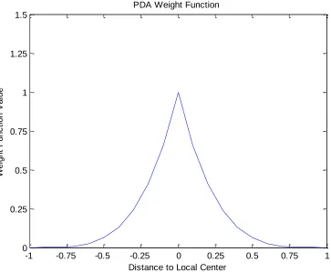
Figure 3.1: Weight function of the reference node with respect to another node where the Distance to Local Center axis is the ratio of the spatial difference over the size of the influence parameter.

-1 -0.75 -0.5 -0.25 0 0.25 0.5 0.75 1

0 0.25 0.5 0.75 1 1.25 1.5

Distance to Local Center

W e ig h t F u n c ti o n V a lu e

the spatial difference to the influence domain size. This figure implies that all nodes that fall within the local influence domain will have a weighting value not equal to zero; where all nodes that fall outside the local influence domain will have a weight value of zero because the radius between the outside nodes and the target node is larger than the influence parameter, therefore making the ratio greater than 1. The weight function used in the PDA is given by

𝑤 (𝐱 − 𝐱̅

𝜌_𝑖 ) = (1 −

‖𝐱 − 𝐱̅‖

𝜌_𝑖 )

4

(3.6) The size of the local influence domain is also important to discuss. This topic will be expanded in chapter 3 but an overview will be addressed in this section. The size of the local influence domain, more formally known as the influence parameter, is a value that determines the node density with respect to the reference node.

In traditional MLSM, the residual is minimized by setting the derivative equal to zero

(𝜕𝐽_𝜕𝐱̅= 0) to yield the following equation

𝐌(𝐱̅)𝐚(𝐱̅) = 𝐁(𝐱̅){𝑢} (3.7)

Where M is the moment matrix and the B matrix is an assembly of p and weight functions defined as

𝐌(𝐱̅) = ∑ (𝐩𝑚(𝐱𝒊; 𝐱̅) ∙ 𝑤 ( 𝐱 − 𝐱̅ 𝜌𝑖 ) ∙ 𝐩𝑚 𝑇_(𝐱 𝒊; 𝐱̅)) 𝑛 𝑖=1 (3.8)

𝐁(𝐱̅) = (𝑤 (𝐱1− 𝐱̅

𝜌1 ) ∙ 𝐩𝑚(𝐱1; 𝐱̅); … ; 𝑤 (

𝐱𝒏− 𝐱̅

𝜌𝑛 ) ∙ 𝐩𝑚(𝐱𝑛; 𝐱̅)) (3.9)

obtain the derivative coefficient matrix, the inverse of the moment matrix must be computed to yield

𝐚(𝐱̅) = 𝐌−𝟏_{(𝐱̅)𝐁(𝐱̅){𝑢} (3.10)}

The invertibility of the moment matrix must be invertible which is only possibly by having a high enough node density around the reference node. The nodal density only depends on one parameter and that is the influence parameter. The larger the influence domain is, the higher the node density will be. By substitution, equation (10) can be rewritten as

(𝐷

𝑟0𝑢(𝑥̅)

⋮ 𝐷𝑟𝑚𝑢(𝑥̅)

) = 𝐌−𝟏_{(𝐱̅)𝐁(𝐱̅) ∙ (}

𝑢1

⋮

𝑢_𝑛) (3.11)

(𝐷

𝑟0

⋮

𝐷𝑟𝑚) = 𝐌

−𝟏_{(𝐱̅)𝐁(𝐱̅) (3.12)}

Equation (12) implies that the inverse of the product of the moment matrix and the B matrix are the actual derivative approximation values. The first row is the 0th derivative approximation and the second row is the first derivative, so forth and so on. These values are substituted directly into the governing differential equation of the reference node to be superimposed into the global shape function matrix. The global shape function matrix can be re-written as

(𝐷

𝑟0𝑢(𝑥̅)

⋮ 𝐷𝑟𝑚𝑢(𝑥̅)

) = [

Φ₁𝑟0 _{⋯ Φ}

𝑛𝑟0

⋮ ⋱ ⋮

Φ₁𝑟𝑚 _{⋯ Φ}

𝑛 𝑟𝑚 ] ( 𝑢1 ⋮ 𝑢𝑛 ) (3.13)

superimposed into a global matrix so that there are an equal number of equations and unknowns.

Application to Solid Mechanics Problems

In the field of solid mechanics, the idea is to obtain the stress, strain and displacement fields of a problem. Extensive research in numerical methods to handle complex problems in solid mechanics have been explored such as modeling permanent deformation, cracks, contact (friction), impact and interface physics. In any solid mechanics problems, each problem is subjected to 3 boundary conditions; the essential boundary condition, the natural boundary condition and the inner domain. The essential boundary condition is a displacement boundary condition in the sense that the displacements are known. The natural boundary condition is the region on the surface of a model where tractions are prescribed. When modeling solid mechanics problems with meshfree numerical methods, each degree of freedom must be subjected to a boundary condition.

The governing equation in linear elastic solid mechanics is given by

𝛁 ∙ 𝛔 + 𝐛 = 𝟎 (3.14a)

Indicial notation (I.N.) will be used for the remaining equations. Equation (3.14a) written in I.N. and given by

∇𝑗𝜎𝑖𝑗+ 𝑏𝑖 = 0 (3.14b)

where 𝜎 is the stress tensor, and b is the body force. For the 1D case, equation (3.14b) is expanded to

𝜕𝜎_𝑥𝑥

𝜕𝑥 + 𝑏𝑥 = 0

For the 2D case, the equation is expanded to

𝜕𝜎𝑥𝑥

𝜕𝑥 +

𝜕𝜎_𝑥𝑦

𝜕𝑦 + 𝑏𝑥 = 0

(3.16)

𝜕𝜎𝑥𝑦

𝜕𝑥 +

𝜕𝜎𝑦𝑦

𝜕𝑦 + 𝑏𝑦 = 0

(3.17)

Stress for linear elastic, homogeneous material is given by

𝜎_𝑖𝑗 = 𝐶_{𝑖𝑗𝑘𝑙}𝜀_𝑘𝑙 (3.18)

The C tensor is more formally known as the elastic coefficient matrix, which is a 4th order tensor given by the following equation

𝐶_{𝑖𝑗𝑘𝑙} = 𝜆𝛿_𝑖𝑗𝛿_𝑘𝑙 + 𝜇(𝛿_𝑖𝑘𝛿_𝑗𝑙+ 𝛿_𝑖𝑙𝛿_𝑗𝑘) (3.19)

And substituting equation (3.19) into equation (3.18) and simplifying yields

𝜎_𝑖𝑗 = 𝜆𝛿_𝑖𝑗𝜀_𝑘𝑘+ 2𝜇𝜀_𝑖𝑗 (3.20)

Where λ and μ are material constants known as Lame parameters. The delta is more formally known as the Kronecker Delta property. The kronecker delta is given by

𝛿_𝑖𝑗 = {1 𝑖 = 𝑗

0 𝑖 ≠ 𝑗}

(3.21)

Equation (3.14) is used for stress analysis for any point within the domain of a problem. The surface tractions are given by the following equation

𝑡𝑖 = 𝜎𝑖𝑗𝑛𝑗 (3.22)

Where t is the tractions at a point and n is the unit normal to a point on the surface. Stress is a function of strain and strain is defined as

𝜀_𝑖𝑗 =1

2(𝑢𝑖,𝑗+ 𝑢𝑗,𝑖)

Where the u denotes displacement at a point. By substituting equation (3.23) into equation (3.20) and substituting equation (3.20) into equation (3.14), the resulting differential equation, also known as the Navier-Lamé Equation, becomes

(𝜆 + 𝜇)𝑢_{𝑗,𝑖𝑗}+ (𝜇)𝑢_{𝑖,𝑗𝑗} + 𝑏_𝑖 = 0 (3.24)

This is the final form in which the differential equation will be approximate by the PDA for all nodes inside the domain. For nodes on the natural boundary subjected to applied tractions and traction-free regions, equation (3.23) will be substituted into equation (3.20) and then equation (3.20) will be substituted into equation (3.22) to obtain a differential form for the traction boundary condition nodes. The final equation will yield

𝑡_𝑖 = 𝜆𝑢_𝑘,𝑘𝑛_𝑗+ 𝜇(𝑢_𝑖,𝑗+ 𝑢_𝑗,𝑖)𝑛_𝑗 (3.25)

CHAPTER

4

C

I

In this section, computer implementation will be discussed. In chapter 3, the PDA was derived and the corresponding equations was presented, however the equations and concepts can be overwhelming and tedious to decipher.

Implementation Concepts.

One of the most important concepts in using this meshfree numerical method with adaptivity is understanding that each node has N degrees of freedom. To be able to solve for these unknown nodal solutions, a system of equations is needed that is n x n where n

is the total degrees of freedom in the overall system. To obtain such as matrix, the PDA will be applied to every node in the system and the matrix will come from the derivative approximations of all nodes with respect to each node.

General Process.

Below are descriptions of how to construct the PDA for linear elastic problems. Each section is listed in order of chronology.

displacements (if on the essential boundary), and surface unit normal (if node is on the surface). The best practice for implementation is the use of data structures for the nodes.

Once the nodal data is obtained, the nodal influence parameters should be computed. This is not part of the discretization process, but should be part of the pre-processing step because these parameters are based on the mathematical modeling data prescribed by the user. There are several methods to compute the influence parameters, but at this point each node needs an influence parameter.

At this point, the pre-processing is complete. This step is the assembly of the shape function matrix where the PDA starts. The PDA process is repeated for each node in the model, in other words, the first node takes the role as the reference point. The reference node, for the purposes of explanation will be denoted as node-i. The M and B matrix need to be computed first by iterating through all nodes in the model, this will be referred to as node-j. To construct the M matrix, the p-vector needs to be assembled. The p-vector follows the Taylor Series Expansion coefficients, for example, 2D quadratic is given by

𝑝𝑇 _{= [1 𝑑𝑥 𝑑𝑦 𝑑𝑥}2 _{𝑑𝑥𝑑𝑦 𝑑𝑦}2_{]. Where 𝑑𝑥 = 𝑥 − 𝑥̅ and 𝑑𝑦 = 𝑦 − 𝑦̅. The x and y are}

the coordinates of node-j where 𝑥 ̅and 𝑦̅ are the coordinates of the reference node, node-i. The weight value is computed as the radial difference between node-i and node-j and if the radial distance is within the influence domain, the weight value will be non-zero. The p-vector and product of the weight value will be placed in the jth _{column of the B matrix.}

with respect to all other nodes, the equation is 𝐷_𝑖0 = [1 0 0 0 0 0]𝑀−1𝐵 for a 2D quadratic system, where 𝐷_𝑖𝑥2 = [0 0 0 2 0 0]𝑀−1𝐵would be the second derivative with respect to x. Once this coefficient array is obtained, each coefficient should be substituted into the governing equation for that node and iterated through the rest of the model nodes and superimposed into the global shape function matrix. For example, consider a 1D

derivative term, 𝑑

2_𝑦

𝑑𝑥2, the coefficient would be 𝐷𝑖2 = [0 0 2]𝑀−1𝐵 and superimposed into

the global shape function matrix in the row corresponding to that node. These derivative coefficient arrays are the actual values of the derivative terms without the value of the unknown function.

Once this process is over, the displacements can be solved. The differential equation coefficients are in the shape function matrix and the RHS of the differential equations consist of the body force terms, tractions and prescribed displacements for the nodes.

At this point the nodal displacements are computed so using the PDA (a derivative approximation method), the nodal strains can be computed because the strains are the derivative of the displacements. Once the strains are known, the stresses can be computed by substituting into the stress equation given back in chapter 3.

CHAPTER

5

N

E

In this section, several numerical examples will be presented. The first two examples are classic examples from solid mechanics will then be presented to show that the PDA is a self-converging system in the sense that globally refining the model will converge the approximate solution to the analytical solution. Then error results for the same two examples will be presented with

Example – Cantilever Beam with Global Refinement

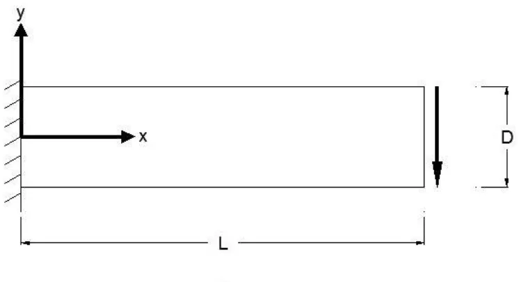
Plane-stress is used because plane-strain is used to model structures that are 1-dimensional in the sense that is has a relatively large dimension in one direction. The assumption for plane stress is that the stress normal to the plane of the domain is 0. Since the domain of the model is given in x and y coordinates, the assumptions associated with plane-stress is that 𝜎_𝑧𝑧, 𝜎_𝑥𝑧, 𝜎_𝑦𝑧are all zero.

Figure 5.1 – Cantilever beam problem with applied traction at end.

Table 5.1 – Parameters for a 2D cantilever beam

Physical Parameter Variable Name Variable Quantity

Length L 64 inches

Depth D 16 inches

Applied Traction P 10 ksi Modulus of Elasticity E 2000 ksi Poisson Ratio v 0.33

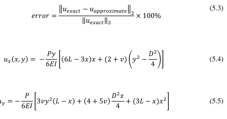
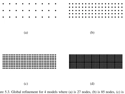
The node discretizations are given by figure 5.3 and the associated error is given by figure 5.4. The error estimate was based on the L2 norm for the nodal displacements and

the equation for the L2 norm is given by

𝐿₂ = ‖𝐮‖₂ = (∑ 𝑢_𝑖2₎1/2 (5.2)

And the error estimator used to compute the error of the approximate solution with respect to the analytical solutions is given by

𝑒𝑟𝑟𝑜𝑟 =‖𝑢𝑒𝑥𝑎𝑐𝑡− 𝑢𝑎𝑝𝑝𝑟𝑜𝑥𝑖𝑚𝑎𝑡𝑒‖2

‖𝑢_{𝑒𝑥𝑎𝑐𝑡}‖₂ × 100%

(5.3)

𝑢_𝑥(𝑥, 𝑦) = − 𝑃𝑦

6𝐸𝐼[(6𝐿 − 3𝑥)𝑥 + (2 + 𝑣) (𝑦2− 𝐷2

4 )] (5.4)

𝑢_𝑦 = − 𝑃

6𝐸𝐼[3𝑣𝑦2(𝐿 − 𝑥) + (4 + 5𝑣) 𝐷2_𝑥

(a) (b)

(c) (d)

Figure 5.4. Cantilever beam relative error of approximate solution with respect to the analytical solution with L2 norm.

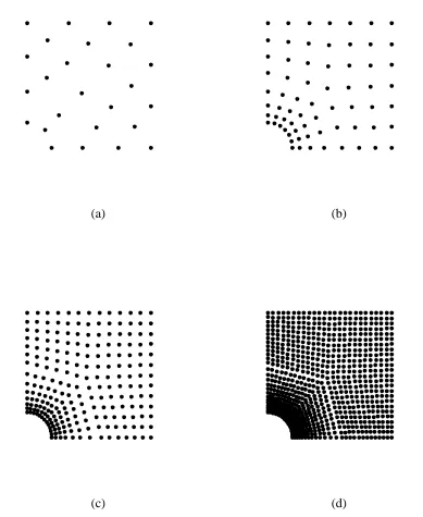
Example – Plate with Hole with Global Refinement

In this example, a plate with a hole at the center will be studied as shown in figure 5.5. The model will only be a quarter-plate with the assumption that each quadrant of the model is equal and opposite as shown in figure 5.6. In the Theory of Elasticity, this class of problem is defined as the infinite plate problem and the analytical solution is given by Timoshenko’s Theory of Elasticity [9] and is represented by equation (5.6, 5.7). It is not possible to model the entire problem due to an unrestrained rigidbody translation. In the model, rollers are used to enforce the condition that the y-axis is non-translational in the x-direction due to symmetry and the x-axis is non-translational in the y-direction as shown in figure 5.7. Table 5.2 gives the parameters of the model and variables as shown in the program. Figure 5.8 shows the relative error with respect to the exact solution and the convergence rate with global refinement.

0 100 200 300 400 500 600 700

0 10 20 30 40 50 60 E rr o r (% )

Table 5.2 – Parameters for a 2D Plate with Hole

Physical Parameter Variable Name Variable Quantity

Length L 5 inches

Applied Traction P 1 ksi Modulus of Elasticity E 2000 ksi Poisson Ratio v 0.33 Radius of Hole a 1 inch

Figure 5.6. The modeling region from the original problem.

(a) (b)

(c) (d)

Figure 5.9. Plate with hole relative error of approximate solution with respect to the analytical solution with L2 norm.

The analytic solutions to the plate with the hole is given by

𝑢𝑟 = 𝑟 (

𝐾 − 1

2 + cos (2𝜃)) +

𝑎2

𝑟 (1 + (1 + 𝐾)cos (2𝜃)) − 𝑎4

𝑟3_4𝐺cos (2𝜃) (5.6)

𝑢_𝜃 = 1

4𝐺(

(1 − 𝐾)

𝑟 𝑎2− 𝑟 −

𝑎4

𝑟3) sin (2𝜃) (5.7)

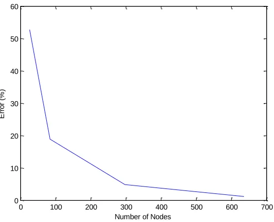
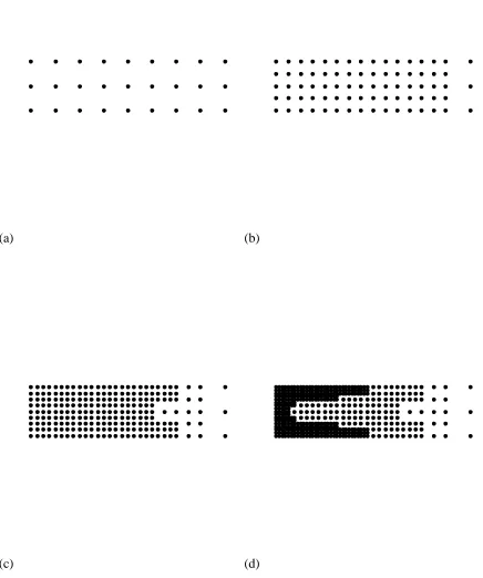
Example – 2D Cantilever Beam with Local Adaptivity

In this section, the 2D cantilever beam problem will be presented with the adaptive approach to show solution convergence without the need of global refinement. All the same parameters will be used, and the adaptivity will be based on the solution of the initial node discretization model containing 27 nodes.

0 100 200 300 400 500 600 700 800 900

0 5 10 15 20 25 30 35 40 45

Nodes in Model

(a) (b)

(c) (d)

Figure 5.11 – Relative error of cantilever beam problem with local node adaptivity.

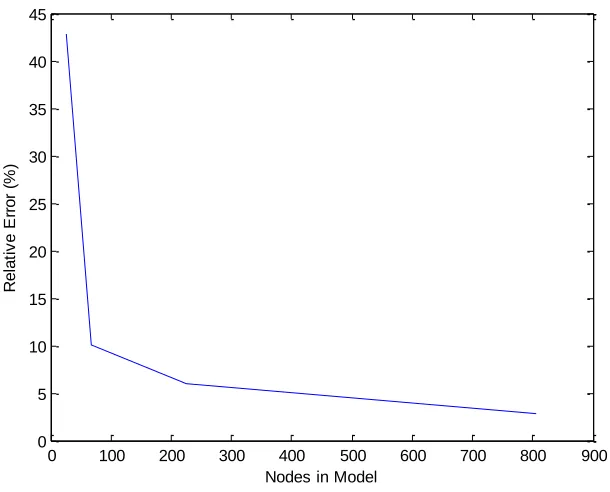
Example – 2D Plate with Hole with Local Adaptivity

In this section, the 2D plate with hole problem will be presented with the adaptive approach to show solution convergence without the need of global refinement. All the same parameters will be used from before and the adaptivity will be based on the solution of the initial node model consisting of 26 nodes.

0 100 200 300 400 500 600 700

0 10 20 30 40 50 60

Number of Nodes

(a) (b)

(c) (d)

Figure 5.13 – Plate with hole relative error based on adaptive process.

0 100 200 300 400 500 600 700 800 900

0 5 10 15 20 25 30 35 40 45 50

Number of Nodes

R

e

la

ti

v

e

E

rr

o

r

(%

)

CHAPTER

6

D

L

I

P

In this section, the influence parameter will be discussed. As mentioned in chapter 2, each node possesses a feature known as the influence parameter. The influence parameter is a radius in which is defines a local influence domain. For the 2D case, the influence domain is a circle and for the 3D case the influence domain is a sphere. The objective of the influence parameter is to be large enough to capture the effects of surrounding nodes to ensure the invertibility of the moment matrix but not too large or the effects of relatively distant nodes could cause the solution to diverge. Kim and Kim [9] devised a dilation function scheme for point collocation meshfree methods, however, their algorithm tends to be unstable for highly irregular node distribution patterns. When implementing their method in an adaptive algorithm, the solution becomes highly sensitive to the 3 input parameters and produces large oscillating errors in a refinement process. In other meshfree methods that implement the MLSM, others have defined the influence parameter to be a constant value, but large enough to satisfy the invertibility criteria such as that in [1].

𝑅 = 𝐶 ∙(𝑚 + 𝑁)!

𝑚! 𝑁! (1)

Where R is the number of required nodes, C is a density coefficient, m is the highest order polynomial and N is the number of spatial dimensions. The algorithm is an iterated process where the initial influence parameter value is the distance to the closets node then an iteration process starts to increase the influence value process until the required

CHAPTER

7

S

C

Meshfree adaptivity methods for point collocation methods are studied. Also a nodal influence parameter algorithm is presented and compared with the dilation parameter function by Kim and Kim [9]. The PDA is different than other point collocation methods because the MLSM derivative approximation is based on a minimized residual functional. Two methods for nodal adaption was presented. The first method was based on a bisection approach in which a node was added between two nodes that resulted in a high change in the gradients. This method is applicable for structured nodal discretizations and rectangular node patterns. The second method is an interpolation approach in which the user defines an acceptable change in gradient and the algorithm adds an appropriate amount of nodes between two high gradient nodes so that the change in gradients are less than or equal to the defined changed in gradient. Several examples were presented ranging from scalar field problems to vector field problems with mixed boundary conditions to show that the proposed adaptive methods allow the approximate solution converge to the analytical solutions, exponentially.

Further Studies

comparisons have been performed to show that adaptivity can be sensitive, and in some cases, highly unstable based on the influence parameter. Figure 9.1 shows the relative error as the number of nodes increase. Recall the proposed influence parameter algorithm requires the user define a radial step size for the algorithm to iteratively increase the radius until the node density is satisfied. Each error plot in figure 7.1 shows the effects of variable radial step sizes. In 7.1 (a), the step size is a constant 2 for each refined model. In 7.1 (b), the step size is a constant 1 for each refined model. In 7.1 (c), the step size is initially 0.5 and decreases linearly by 0.1 until the end of the refinement process. In figure 7.1 (d) the radial step size is the square root of 1 to account for nodes along a square diagonal. These are just a few examples of how significant the effects of the radial step size are in the refinement process.

Other mathematical approaches can be used for the adaptivity process. In meshed methods, the 3 types of adaptivity approaches are H-adaptivity, P-adaptivity and L-adaptivity. For meshfree methods, H- and P-adaptivity is generally accepted, however the L-adaptivity is not. Recall L-adaptivity for meshfree methods is the process of moving nodes to have better coverage in regions of high gradients, but this is not acceptable in meshfree methods because the initial points are typically defined at locations where information is critical such as places where boundary conditions exist or tractions are applied. Certain points cannot be moved also due to the node density criteria and having irregular influence parameters that could cause instability in the adaptive methods.

(a) (b)

(c) (d)

Figure 7.1 – Relative error as a function of node count based on different influence parameters. (a) is the solution based on the proposed dilation function by [9], (b-d) is the proposed influence parameter based on variable K values.

0 100 200 300 400

0 100 200 300 400 500

Number of Nodes

E rr o r (% )

0 100 200 300 400 500

10 20 30 40 50 60

Number of Nodes

E rr o r (% )

0 200 400 600 800

0 20 40 60 80 100

Number of Nodes

E rr o r (% )

0 200 400 600 800

0 10 20 30 40 50 60 70 80

Number of Nodes

R

1. T. Belytschko, Y. Lu, L. Gu, “Element-Free Galerkin Method”, International Journal for Numerical methods in Engineering, 37:229-256 (1994).

2. Y. Yoon, J-H Song, “Extended Particle Difference Method for Weak and Strong Discontinuity Problems Part I.”, Computer Methods in Mechanics, 53:1087 – 1103 (2014).

3. J. Oden, S. Prudhomme, “Goal-Oriented Error Estimation and Adaptivity for the Finite Element Method”, Computers and Mathematics with Applications, 41:735-756 (2001).

4. T. Rabczuk, T. Belytschko, “A Three-Dimensional Large Deformation Meshfree Method for Arbitrary Evolving Cracks”, Computer Methods in Applied

Mechanics and Engineering, 196:2777-2799 (2007).

5. T. Rabczuk, T. Belytschko, “Adaptivity for Structured Meshfree Particle Methods in 2D and 3D”, International Journal for Numerical Methods in Engineering, 63:1559-1582 (2005).

6. L. Ling, “An Adaptive-Hybrid Meshfree Approximation Method”, International Journal for Numerical Methods in Engineering, 89:637-657 (2012).

8. C. Augarde, A. Deeks, “The Use of Timoshenko’s Exact Solution for a Cantilever Beam in Adaptive Analysis”, Finite Elements in Analysis and Design, 44:595-601 (2008).

9. D. Kim, H. Kim, “Point Collocation Method Based on the FMLSRK Approximation for Electromagnetic Field Analysis” IEEE Transactions on Magnetics, 40 (2004).