Impedance Analysis of A Foundation Supported on A Sloping Layered Soil

(1)

Impedance Analysis of a Foundation Supported on a Sloping Layered Soil

Yoshio Ikeda 1) and Hiroshi Tajimi 2)

1) Nuclear Facilities Dept., Eng. Div., Taisei Corporation, Tokyo, Japan 2) Tajimi Engineering Services, Ltd., Tokyo, Japan

A B S T R A C T

The present paper aims to obtain a dynamic impedance of a foundation supported on a horizontal surface which was made by cutting a sloping formation consisting of laminated soils. The analysis uses the direct boundary integral method applied to a half-space analogy with an excavation as an exterior problem. The soil model is assumed in accordance with the thin-layer approach. Since this model is treated as lying horizontally, the foundation is rather inclined. The evaluation of traction matrix is reasonably improved. Main interests are laid on variation of the impedance of foundation with soil profiles and in addition with the effects of inclination of supporting soil layers.

I N T R O D U C T I O N

The present paper aims to obtain a dynamic impedance of a foundation supported on a horizontal surface which was made by cutting a sloping formation consisting of laminated soils. Special interests are laid on the variation of impedance with the soil profiles.

The analysis treats the 3-dimensional thin-layer model, which consists of a horizontally laminated medium and is characterized by use of linearization of the displacements in the layering direction, while it is assumed as a continuum in the lateral direction. This model is well known by its application to the formation of transmitting boundary [1]. Afterwards, the Green's functions of the model have been developed in

[2],[3],[4] and are now essential to their application in the BEM analysis. Fig.1 Configuration of analytical object F U N D A M E N T A L S O L U T I O N IN T H E THIN-LAYER M O D E L

Consider a thin-layer model consisting of N layers. When a point excitation of

(Px, Py, Pz)

is applied to the origin of the s-interface, the resulting displacement of (u, v, w) at the location of (r, 0 ) of the r-interface is given in the following forms:

u V 1 cos 20 + V 2 V 1 sin 20 V 4 cos O

Px

w = V ls i n 2 0 -V 1 c o s 2 0 + V 2 V 4sin0

Py

- V 3 cos 0 - V 3 sin 0 V5 Pz

(1)

1 XrkXsk 2

1 N yrkYsk Fl(flkr)

V1 =-2---~ k=l

Dkot

ak Fl (C~k r) +-~Z = Dkp

12~k l XrkXsk 2

l ~ YrkYsk F2(flkr )

Fig. 2

V 2 - - ' ~ =

Dka

a i F 2 ( a ~ r ) + ' ~ z k=l

DkP

=__~1 ZrkXsk 2

1 2~k 1XrkZsk 2

.___1 ~ZrkZsk 2

V3 Z k=l

Dta

°~iF3(°~kr)' V 4 - 7 =

Dka

o~kF3(o~kr)' V5 /r k=l

Dta ~iF2(~kr)

F~ (g') = - ~ + ~ H (2> (g'), F 2 (g') = ~- Ho (2> (g'), F 3 (g') = -~ H (a> (g')

! I

Py

s s SS

P~

Coordinate system of a thin-layer model

H~ 2) (z)=Hankel function of the 2nd kind

SMiRT 16, Washington DC, August 2001 Paper # 1381

(2)

In the above, o~ k and

(Xrk,Zrk), (Xsk,Zsk)are

eigenvalues and eigenvectors, respectively, as solutions of the quadratic equation of Rayleigh wave mode. Similarly, flk and

Yrk, Ysk

are eigenvalues and eigenvectors, respectively, as solutions of the quadratic equation of Love wave mode.

D m

and

Dkp are

the corresponding modal coefficients.

T R A C T I O N MATRIX USED TO THE BEM ANALYSIS

The traction-displacement relationship in a single thin layer can be defined by those at two nodes in the top and bottom surfaces of a layer and is given by

(2)

The analogous relationship in a layer system is expressed by those of any two contacting layers and can be written as

Fig. 3 i-1

t1

;+1

1

Boundary elements

Ipi-1

-k~l 1

k~21

Iui-1

p i = kill ki-21 +k[ 1 k[ 2 l

ui

pi+l

k~ 1

ki22 ui+l

(3)

Eq.(2) can be obtained by the well known virtual work method and its general form is given in the text as

k = I B r D B d(vol)

(4)

where D denotes the elasticity matrix connecting the stress o" and strain e in the form

a = D e

(5)

m

and B denotes the transformation matrix connecting the strain e to the relevant derivatives V of displacements from the fundamental solution of Eq.(1) in the form

m

e = BV

(6)

Herein, B is given by [5]

B = L N (7)

In these equations, one has

(8a)

I bu Ov Ow ~u Ov by

~

~ - t - ~ ~-~-~

e= -~x Oy ~9z Oy ~gx Oz

Ow Ow Ou

₊

_j

_(8b)

a y a x - ~ z

D

~,+2G ~ ,~

,,~ ~,+2G

A & + 2 G G

G G

(8c)

(3)

. . . . . . . u v w 7

Ox ~x ~y ~y ~z H H

-l~'-[Z x Zy Zz]

LX 1 0 0

0 0 0

0 1 0

0 0 0

_0 0 1_

Zy =

-0 0 O"

0 1 0

0 0 0

1 0 0

[ 01

0 0

, L z =

-0 0 0-

0 0 0 0 0 1 0 0 0

(9)

(lOa)

(lOb)

N=EN1 N2]

(11a)

Sl

=diag(H ZH ZH ZH ZH

z 1 H 1 1)

N2=diag( 1-zH 1-ZH 1-!H 1-ZH 1-ZH 1-ZH -1 -1 -1 !

(llb)

(llc)

It follows that the traction P = [P1 /'2 ] working on the width

wf

of the element and the corresponding derivatives of displacement 1 7 = [ ~ 179 ] are combined by

[o ]_- sr ]

A = -~DE

(12)

where the components of vectors of traction and displacement are

[ L

i

ilT"

Pi = P Pxy Pxz Pyx Pry Pyz Pzx Pzy Pzz ,

_i..

Vi = ~tli ~vi .~i ~"i ~ i ~12i bli Vi Wi

i=1, 2 (13a)

(13b)

Finally, one has the stiffness matrix in the form,

k = d z = w f

wf a i ~ ~ A ~ 1

Nf AN 2

C21 C22

wf =

width of the concerned face of the element

(14)

The detailed results of Eq.( 14 ) are presented in Appendix.

BOUNDARY I N T E G R A L AROUND A HALF-SPACE ANALOGY WITH AN EXCAVATION

As well known, the BEM analysis treats the integral:

u k

(x, co) --

~aD Uki(X' Y'co)Pi(Y'co)ds(y)- faD wki(x' Y'co)ui(Y'co)ds(y)

(15)

If the source point x within the domain D approaches to a boundary point y on OD, the traction

Wki

(x,y,co)

becomes more strongly singular and must be evaluated by the Cauchy principal value. But this method is applied to only

(4)

the interior problem, while the exterior problem is usually solved by the following method:

u k (x,w) = f Uki(x, y,w)pi(y,w)ds(y)- f Wki(x , y,w)(ui(y,o))-ui(xo,w))ds(y )

,I bD ,I bD

-- U i ( Xo , O9) rOD w k i ( x '

y, (o)ds(y )

(16)

where x 0 means the source point laid on the boundary. In thus rewrited expression, the 2nd term in the right-hand side

holds finite and regular, even if

Ix-yl ~ O.

However, the 3rd term shows strong singular. In the 2nd term, since

Wki(x,y,(o )

is given by a product with

ui(y,o) ) ,

its contribution to the integral can be neglected, because

ui(y,oo )

vanishes at the laterally infinite boundary as well as at the lower boundary of the model. But, the 3rd term can not be neglected.

~D ~D 1 bD 2

,

,I

,

,,

. ... . ... ...

,

I I I I I I

i i I i i ... i

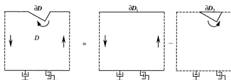
Fig. 4 Integration contour of a thin-layer model with an excavation

The exterior domain D herein considered can be taken as the space which is covered entirely by the thin-layer model D 1 and partially subtracted by the excavation zone D 2 .

Therefore, one has

f ~D = f ~DI --~~D2

(17)

If the thin-layer model is made to simulate to the half-space, one can approximate

f,

Wki(x, Y,W)ds(y) = l

(18)

OD1

According to the Gauss divergence theorem, the boundary integral of

Wki (x, y, w)

in the domain D 2 is given by the

volume integral of the equilibrium equation of stresses

O'ig

with the applied force as well as the inertia force, so that one can

write

~~D2 Wki(x'Y'O))ds(y)= fv2[(O'ik'i-piii)-6kiS(x°-Y)-pii(xo)ldv(y)

(19)

where Ui is the relative acceleration to the surrounding acceleration //(x0) and the second term represents the applied unit

force. The fundamental solution to be substituted herein vanishes the equilibrium equation of the internal stresses. It means

to make the first term in the parenthesis to be null, so that it yields

f

Wki(x, y,w)ds(y) =-

Io

6ki6(x- y)dv(y)+

fo

pro2Uki(x, y,w)dv(y)

(20)

OD2 2 2

When this equation is substituted into Eq.(17), the traction forces

Wki(x,y,(O )

on both interior and exterior

boundaries should be noticed to be different each other in their signs of + , one obtains

J

Wki(x, y,w)ds(y) = l -

fo,

6ki6(x- y)dv(y)+

fo

pW2Uki(x, y,w)dv(y)

OD1 1

(21)

(5)

uk ( X' CO) - uk ( X°' CO) = ~bD U ki ( x' Y' co) Pi (Y' co) ds( y ) - ~oDWki ( x' Y' g-°)(ui (Y' (°)- ui ( x°' g-°)) ds( y )

_ui(Xo,co)Ii+~~DP(O2Uki(x,y, oJ)dv(y)]

(22)

If x approaches to x 0, the left-hand side of the above equation vanishes and it produces the following boundary

integral equation:

~OD

Uki

(X0'

y' co)Pi (Y, co)ds(y) - f ~o Wki (x°' y' co)(Ui (y' co) -- bli (XO'

0 =

co))ds(y)

-ui(Xo,co)II+~bDPco2Uki(xo,Y,co)dv(y)]

(23)

For the numerical integration, one uses the constant elements and rewrite the above equation into the discrete forms as N

I' Uki(x°' Y'co)Pi(Y'co)ds(y) ---> Z UkiPi

bD ₁

N

Wki(xo, Y, co)ui(Y,co)ds(y ) --->

WkiU i

1

(24)

u

where it should be noted that the diagonal component W~ in the traction matrices Wki is specified as the following form in accordance with Eq.(23 ):

N2 N

Wkk - I + Z p c o 2 U k i V i - Z W k j ( 2 5 )

i k~j

Vj =

volume occupied by the node j, N 2 = total number of nodes in D 2

N U M E R I C A L E X A M P L E S

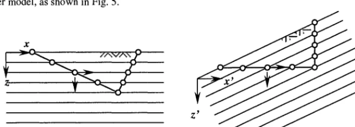
The analysis requires the rotation of the prototype model so as to agree the sloping surface with the horizontally free surface of the thin-layer model, as shown in Fig. 5.

X

Z ~

Fig. 5 Coordinate axes of analytical model and prototype model

(6)

The present paper emphasizes the methodology for solving the impedance of the foundation placed in the excavation of the layered soils. The above numerical works have been conducted to illustrate its applicability. While the results are limited to only the case that the foundation is placed closely to the surrounding excavation wall, the following conclusion may be drawn:

1. The static values of the horizontal stiffness decreases slightly as the inclination angle increases, while those of the rocking and vertical stiffnesses increase with increasing of the inclination angle.

2. The top stiffer soil profile seems to affect the rocking impedance rather than the horizontal impedance.

REFERENCES

APPENDIX

1. Waas, G., "Linear Two-Dimensional Analysis of Soil Dynamics Problems in Semi-Infinite Layered Media," Ph.D. Thesis, Univ. of California, Berkelery, California, 1972.

2. Tajimi, H., "A Contribution to Theoretical Prediction on Dynamic Stiffness of Surface Foundations," Proc. 7th World Conf. Earthquake Eng. Istanbul, Vol.5, pp.105-112, 1980.

3. Kausel, E., "An Explicit Solution for The Green Functions for Dynamic loads in Layered Media," MIT Research Report r81-13, Department of Civil Engineering, MIT, Cambridge, Ma, 1981.

4. Tajimi, H., " Predicted and Measured Vibrational Characteristics of a Large-Scale Shaking Table Foundation," Proc. 8th World Conf. Earthquake Eng., San Francisco, Vol. III, 873-880, 1984.

5. Kausel, E., "Thin-Layer Method: Formulation in the Time Domain," Int. J. Numer. Math. Engng., Vol. 37, 927-941, 1994.

Cll

The C matrix in Eq.(14) is given by

C21

I 2Axx 2Axy 3Axz

Axx

Axy -3Axz

H I2Ay x 2Ayy 3Ay z

H

= "-6-- ' C12 = ~ Ayx Ayy - 3 A y z

[ 3Azx 3Azy 6Azz

3Azx 3A~ -6Azz

A ~ - -

I

Axx

Axy

3Axz

H | 2Ay x

,r

2A~

2Axy

2Ayy

= H Ay x

Ayy

3Ay z ,

C22=

6 L -3Azx -3Azy "6Azz 1-3azx -3azy

-3Axz

-3Ay z

6Azz

2 + 2 G

A ~ - G ,

G

2 + 2 G 2

G , A x z =

G

2,

G

Ayx= A

G

Ayy =

G

, Ayz =

G

2 Azx

G

A

Azy --

G

G ,

Azz =

~,+2G

CONCLUSIONS

(7)

Nodal Surface No.

1

9 --;

/

10 _/z. 1 1 / -

/

12 -7

/

13 /'~

14 -z--..._ /

/ 15 " ~

16

17

18

_/

J

/

19 /

20 21 22 23 24 25 35 36 i / / /

/--7

/

,4,..,. i i i

/

/ ~3 /

/ / 8 0 . 0 m /

/ ,,,' / ,,

/

/ / / / / / /

/

/ / /; / / i i / i

/

t a n ¢~ = 0 . 4

/

--or

i

- p - - -

/

j//

..z. / / _¢.. / / . - . z .

/

=.4===== /

/

/ / / ! / ,,: i

1. O / / i / / /

' , ' 4 " -

/ /

6

/ / )..._

-'-'-4, !

...¢., / ! .._.,L / / / ---O--- / / / / / / ¢ / / /

/

30.0 m

Case 1 Case 2 A . . .

/

~ B A

m

A

I

lO.O m

v~

m/s

A 2000

B 1300

P kNs2/m 4 2.67 2.01 0.36 0.35 / - . 4 . =

/

,i,

O m

40 m

lOOm

250 m

(8)

( X 1 0 9)

2 . 0 . . . . , . . . . , . . . . , . . . . , . . . .

1.5

Z

,.~ 1 . 0

0 . 5

t~

~, 2 . 0

Z

~, 1.0

R e . tan ¢ = 0 . 0

- - - - . . - - - tan ¢ = 0 . 2

. . . . tan ~ = 0 . 4

. , . i , , . , , - - , , - , , . . ~ - - , ~ - ~ ' - " ' ' ' ' '

O 0 .. .. I .... I • i f , I , i i i i ! i i s

O. 2 4 6 8

F r e q u e n c y ( H z ) ( X 1 0 1 2 )

3 . 0 . . . . , . . . . , . . . . , . . . . , . . . .

R e . tan ~ =0.0

- - - tan ~ =0.2

. . . . tan ~ =0.4 1 0

__ __ - - ~ _ .

0 . 0 0 . . . 2 4 6 8 1 0

F r e q u e n c y ( H z )

Z 1.0

0 . 5

( X 1 0 9 )

2 . 0 . . . . , . . . . , . . . . , . . . . , . . . .

l m . tan ~ =o.0

- - - - . - - - . tan ~ =0.2 1.5

. . . . tan ~ = 0 . 4

0 . 0 0

.. .. I ... . I .... I .... I ....

2 4 6 8 1 0

F r e q u e n c y ( H z ) ( X 1 0 1 2 )

2 . 0 . . . . , . . . . , . . . . , . . . . , . . .

I m . tan ~ =0.0

- - - tan ~ = 0 . 2

1.5

¢~ tan ~ = 0 . 4

Z 1.o

0 . 5

0 0 o ' I ~ - ' T i " - ' " 2 r ' 4 . . . . 6' . . . 8

_ _ . . ~ D i b ~ . . . - ~ . v

10 F r e q u e n c y ( H z )

F i g . 7 R e a l a n d i m a g i n a r y p a r t s o f h o r i z o n t a l a n d r o c k i n g i m p e d a n c e f u n c t i o n s , C a s e 1, H o m o g e n e o u s s o i l

Z

..~ 1.0

0 . 5

( X 1 0 9)

2 . 0 . . . . , . . . . , . . . . , . . . . , . . . .

R e ,

v

~ ~ ' ,=

1.5 . ~ ~ ~ - - = - - ~

"o

0 . 0 0

~ i ~ O ~ ° ~ I ~ t / l ~ 0 ~ ~j i j i j II e j j l n l ~ j ee ~

, tan ~ = 0 . 0 - - - tan ~ = 0 . 2 . . . . tan ~6 = 0 . 4

I I ' ' I .. .. I , I , I .... I .. ..

2 4 6 8

F r e q u e n c y ( H z ) ( X 1 0 1 2 )

3 . 0 . . . . , . . . . , . . . . , . . . . , . . . .

R e .

2 . 0

Z - - - ~ ~ ~ . : . _ . _ . . - . ~ 2 2 ~ - ~ ~ - - . -

1 0

1 . 0 ~ tan ~6 = 0 . 0 - - - tan ~ = 0 . 2 . . . . tan ~ = 0 . 4

0 " 0 0 . . . 2 . . . . 4 . . . . ; . . . . 8 . . . . 10

2 . 0

1.5

Z

( X 1 0 9 )

l m . tan ~ = 0 . 0 - - - tan ~ = 0 . 2 . . . . tan ~ = 0 . 4

.... ! ....

o . o . . . . ; . . . . ; " 1 o

2 . 0

1.5

2; 1.0

0 . 5

F r e q u e n c y ( H z ) ( X 1 0 1 2 )

. . . i . ... i .... i . ... j

I m . tan ~ = 0 . 0 tan ~ = 0 . 2 . . . . tan ¢ = 0 . 4

° , f ' /

. . . . . . . ; . . .

0 " 0 6 . . . . 2 8 10

F i g . 8 R e a l a n d i m a g i n a r y p a r t s o f h o r i z o n t a l a n d r o c k i n g i m p e d a n c e f u n c t i o n s , C a s e 2 , T o p s t i f f e r s o i l p r o f i l e

}