ABSTRACT
JASPER, MICAH NATHANAEL. Development and Application of the DIRECT Algorithm for Leak Detection in Water Distribution Systems. (Under the direction of Dr. Kumar
Mahinthakumar).
The Dividing Rectangles (DIRECT) search is a deterministic, global search algorithm for bound constrained problems. The algorithm searches for the global minimum by
recursive space partitioning, essentially grouping similar regions in the decision space and selecting a sample from each group. The DIRECT algorithm was initially designed for continuous problems, but has since been modified to allow for integer variable types.
This research extends the DIRECT algorithm to use a mix of continuous and discrete variables, including connected graph nodes. The algorithm is first tested with standard test functions and then applied to leak detection problems in water distribution systems (WDSs), which involve both discrete network nodes and continuous magnitudes. In addition, the DIRECT algorithm is parallelized using a master-worker paradigm and tested using cluster resources for a moderate number of processors.
The extension of DIRECT algorithm to problems involving discrete network
Development and Application of the DIRECT Algorithm for Leak Detection in Water Distribution Systems
by
Micah Nathanael Jasper
A thesis submitted to the Graduate Faculty of North Carolina State University
in partial fulfillment of the requirements for the degree of
Master of Science
Civil Engineering
Raleigh, North Carolina 2014
APPROVED BY:
DEDICATION
I dedicate this thesis to my wife, my bestest best friend, and something more, Christian Ashley Jasper. C-:
BIOGRAPHY
ACKNOWLEDGMENTS
First and foremost, I would like to thank God from whom all blessings flow, such as life, breath, a beating heart, and many other things that I take for granted (James 1:17). It is through our Lord Jesus that all things are possible (Mark 9:23) and it is He who is able to do immeasurably more than all we ask or imagine (Ephesians 3:20).
I would like to thank my advisor, Prof. Kumar for his help with the C coding, EPANET, and MPI. He is very knowledgeable about high-performance computing and inverse modeling, and he greatly aided this research. I would like to thank Prof. Ranjithan for encouraging me to go to graduate school when I was still taking undergraduate classes at NC State. I would also like to thank Prof. Brill for his encouragement through this research and for giving me the opportunity to TA his Engineering Economics class, probably my favorite engineering class. I would also like to thank my committee members for their feedback and discussion in the group meetings over the past two years. Thank you for your encouragement and advice.
I would also like to thank Jörg Gablonsky, Daniel Finkel, and Prof. C. T. Kelly who were students and faculty here at NC State, whom I have never met, but whose research on the DIRECT method greatly helped my understanding of the algorithm.
Thank you to the National Science Foundation and the Civil Engineering Department at NC State for funding this research.
TABLE OF CONTENTS
LIST OF TABLES ... ix
LIST OF FIGURES ... x
Chapter 1 Introduction ... 1
1.1 The DIRECT Algorithm ... 1
1.2 Leak Detection in Water Distribution Systems ... 3
1.3 Overview ... 3
Chapter 2 The Original DIRECT Algorithm ... 4
2.1 Definition of Lipschitz Continuous ... 4
2.1.1 Examples of Lipschitz continuous functions ... 5
2.1.2 Examples of Continuous Functions that are not Lipschitz Continuous ... 5
2.2 Lipschitz Optimization in One Dimension ... 6
2.2.1 Algorithm Steps ... 7
2.2.2 One Dimensional Example ... 7
2.2.3 Disadvantages of Lipschitz Optimization ... 9
2.3 DIRECT Algorithm in One Dimension ... 9
2.3.1 Division in One Dimension ... 9
2.3.2 Potentially Optimum Intervals ... 11
2.3.3 ε Parameter ... 14
2.3.4 Algorithm Steps ... 15
2.3.5 One Dimensional Example ... 17
2.4 DIRECT Algorithm in Two or More Dimensions ... 19
2.4.1 Normalization to a Unit Hypercube ... 19
2.4.2 Division in Two or More Dimensions ... 19
2.4.3 Rectangle Size ... 21
2.4.4 Algorithm Steps ... 22
2.4.5 Two Dimensional Example ... 23
2.5 Changes to the DIRECT Algorithm from Prior Research ... 24
2.5.1 Aggressive DIRECT ... 24
2.5.2 Dividing Only One Dimension ... 25
2.5.4 Only One Minimum Rectangle per Size Group ... 28
2.5.5 Integer Variables ... 29
2.5.6 Adaptive ε Parameter ... 30
Chapter 3 The DIRECT Algorithm for the Generic Variable Type ... 32
3.1 Generalized Variable Type ... 32
3.1.1 Division ... 33
3.1.2 Midpoint ... 35
3.1.3 Singularity ... 35
3.1.4 Copy ... 35
3.2 Generalized Rectangle ... 36
3.2.1 Division ... 36
3.2.2 Midpoint ... 37
3.2.3 Singularity ... 37
3.2.4 Radius ... 37
3.3 Test Functions ... 38
Chapter 4 Leak Detection in Water Distribution Systems (WDS) using the Dividing Rectangles (DIRECT) Search ... 40
4.1 Introduction to Leak Detection ... 40
4.1.1 Motivation ... 40
4.1.2 Current Approaches ... 40
4.2 Water Distribution Simulator ... 41
4.2.1 Leak Representation... 42
4.2.2 Inverse Modeling Approach ... 43
4.2.3 Objective Function ... 44
4.3 Dividing the Discrete Network Nodes ... 45
4.4 Problem Representation ... 46
Chapter 5 Leak Detection Results... 47
5.1 Small Network ... 47
5.1.1 DIRECT Options Tests ... 49
5.1.2ε Parameter Tests ... 52
5.1.3 Location and Magnitude for Small Network (Method 1) ... 54
5.2 Large Network ... 59
5.2.1 Location and Magnitude for Large Network (Method 1) ... 61
5.2.2 Magnitude at Candidate Nodes for the Large Network (Method 2) ... 63
5.3 Comparison of the DIRECT algorithm and a Genetic Algorithm ... 65
Chapter 6 Parallel Performance ... 67
6.1 Parallel Organization ... 67
6.2 Computer Architecture... 68
6.3 Speedup Curves for Different DIRECT Options ... 69
Chapter 7 Conclusions and Future Work ... 72
7.1 Summary ... 72
7.2 Future Work ... 73
REFERENCES ... 75
APPENDICES ... 77
LIST OF TABLES
Table 3.1 - General Variable Interface ... 33
Table 3.2 - Possible Division Procedures for Various Variable Types ... 34
Table 3.3 - General Rectangle Interface ... 36
Table 3.4 - Function Evaluations to find Global Minimum for Test Functions ... 39
Table 5.1 - Comparison of DIRECT Options for Low Dimensional Problems in Terms of the Number of Function Evaluations to Find the True Leak Case ... 51
Table 5.2 - Comparison of Aggressive DIRECT Options for Low Dimensional Problems in Terms of the Number of Function Evaluations to Find the True Leak Case ... 51
Table 5.3 - Comparison of Various ε Parameters using Method 1 for Low Dimensions in Terms of the Number of Function Evaluations to Find the True Leak Case ... 53
LIST OF FIGURES
Figure 2.1 - Lipschitz continuous function, with Lipschitz constant K, such that for any point within the domain, the slope is within ±K ... 4 Figure 2.2 - Functions that are Lipschitz continuous over the real domain ... 5 Figure 2.3 - Functions that are not Lipschitz continuous over the real domain ... 5 Figure 2.4 - First Iteration of Lipschitz Optimization with the Objective Function Estimate,
B, shown for the Interval [a, b] ... 6 Figure 2.5 - One Dimensional Example of Lipschitz Optimization ... 8 Figure 2.6 - Comparison of Lipschitz and DIRECT Divisions ... 10 Figure 2.7 - Graphical interpretation of "potentially optimal" interval selection, with
intervals represented as points, and the "potentially optimal" intervals along the delineated convex hull ... 11 Figure 2.8 - Graphical interpretation of Lipschitz interval selection, with the Lipschitz
constant, K, represented as a line, and the selected interval as a point along this line ... 13 Figure 2.9 - Graphical interpretation of DIRECT interval selection with ε Parameter
illustrated as a slope and the "potentially optimal" intervals delineated along the modified convex hull ... 15 Figure 2.10 - Rectangle Storage for Potentially Optimal Determination ... 16 Figure 2.11 - One Dimensional Example of DIRECT Optimization ... 18 Figure 2.12 - DIRECT sampling and division in two dimensions with the objective function value shown above each point ... 20 Figure 2.13 - Objective Function for Two Dimensional DIRECT Example ... 23 Figure 2.14 - Two Dimensional Example of DIRECT Optimization ... 24 Figure 2.15 - Graphical interpretation of the rectangle selection using Aggressive DIRECT
Figure 5.2 - Final Objective Function Value for Various Leak Configurations for the Small
Network using Method 1 ... 54
Figure 5.3 - DIRECT Solution for 3 Leaks Searched For and 1 Actual Leaks "3 1" ... 55
Figure 5.4 - DIRECT Solution for 3 Leaks Searched For and 3 Actual Leaks "3 3" ... 55
Figure 5.5 - Final Objective Function Value Comparison for the Small Network using Method 1 ... 57
Figure 5.6 - DIRECT Solution for 6 Candidate Nodes and 2 Actual Leaks "6 2" ... 58
Figure 5.7 - DIRECT Solution for 6 Candidate Nodes and 6 Actual Leaks "6 6" ... 58
Figure 5.8 - Actual and Candidate Leak Locations for the Large Network (Network_2) ... 60
Figure 5.9 - Final Objective Function Value Comparison for the Large Network using Method 1 ... 61
Figure 5.10 - DIRECT Solution when Searching for 3 Leaks with 3 Actual Leaks "3 3" ... 62
Figure 5.11 - Final Objective Function Value Comparison for the Large Network using Method 2 ... 63
Figure 5.12 - DIRECT Solution with 6 Candidate Nodes and 6 Actual Leaks in the Large Network "6 6" ... 64
Figure 5.13 - GA Comparison for Small Network using Method 1 ... 66
Figure 5.14 - GA Comparison for Small Network using Method 2 ... 66
Figure 5.15 - GA Comparison for Large Network using Method 1 ... 66
Figure 5.16 - GA Comparison for Large Network using Method 2 ... 66
Figure 6.1 - Simple Parallel Implementation ... 68
Chapter 1 Introduction
The Dividing Rectangles (DIRECT) search is a deterministic, global search algorithm for bound constrained problems [1]. This method is able to locate areas around local optima in relatively few function evaluations, but it takes many more function evaluations to
converge around a global optimum [2].
The DIRECT method was originally designed for continuous problems. The
algorithm has since been modified to allow for integer problems [3]. However, the DIRECT method has not been applied to other discrete variable types, such as graph nodes. Part of this research is generalizing the DIRECT algorithm to allow for all possible variable types as long as the decision space can be intelligently grouped or divided, and as long as each group or section can be representatively sampled.
Furthermore, the DIRECT method has not previously been applied to problems involving a water distribution system (WDS). A second aim of this research is evaluate the feasibility of solving for the location and magnitude of leaks in a water network using the DIRECT search.
1.1 The DIRECT Algorithm
The DIRECT method is typically used for problems with bound constraints (also called box constraints), meaning that each of the decision variables has a minimum and maximum values, but no other constraint equations. However, the DIRECT algorithm has been later modified to allow for other kinds of constraints [2] [3].
Furthermore, the DIRECT method is considered to be a sampling algorithm, or a derivative-free method, because it does not use the derivative of the objective function. This is particularly useful in engineering applications and other difficult problems where
information about the function, such as the smoothness, continuity, and differentiability, is not available. Often times in engineering problems, the objective may be the product of a simulation or some other iterative method. This also means that it can be computationally expensive to calculate the objective, taking many minutes, hours, or even days. Therefore, it is preferable in many engineering problems to use an algorithm that takes few function evaluations and is easily parallelizable.
The DIRECT algorithm takes relatively few function evaluations when compared to other methods [1], and can be parallelized [2] [4] [5] [6], though the number of function evaluations does change per iteration. It has also been noted that the DIRECT method does not scale well in higher dimensions [3] [7]. This is a problem for some engineering
1.2 Leak Detection in Water Distribution Systems
Water distribution systems (WDSs) are critical in transporting safe, clean drinking water to the public. Yet, these systems age and degrade, and are thus vulnerable to leaks. It has been estimated that up to 50 percent of water in a WDS is lost to leaks [8].
There are many current ways of detecting leaks. Equipment called acoustic listening devices that can detect the sound of water flowing through a crack in the pipe, like a
stethoscope for pipes. Other methods include inverse transient analysis, infrared imaging, and tracer gas analysis. Most of the current methods are time and labor intensive. The goal of this research is to aid in the location of suspect leak areas by using measurements that can be routinely taken, such as the pressure and chlorine concentration at specific nodes, and the flows through certain pipes. These measurements can be used in an inverse modeling
approach, specifically a simulation-optimization approach, using EPANET a WDS simulator, to solve for the location and magnitude of leaks.
1.3 Overview
Chapter 2 The Original DIRECT Algorithm
The DIRECT algorithm is considered a Lipschitzian optimization algorithm, even though it bears only a slight resemblance to the original Lipschitz optimization.. It was originally designed to overcome some of the pitfalls of traditional Lipshitz optimization [1]. This chapter details the origin of the DIRECT algorithm and some modifications since. 2.1 Definition of Lipschitz Continuous
A function is considered Lipschitz continuous if the slope of the function is not greater in magnitude at any point in the domain than a finite constant. More formally, a function is Lipschitz continuous if and only if there is a positive constant K, called the Lipschitz constant, such that
|f(x1) - f(x2)| ≤ K|x1 - x2|, for all x1 and x2 in the domain X
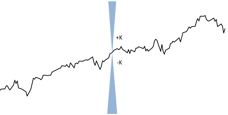
A function that is Lipschitz continuous over a specified domain is shown in Figure 2.1.
Figure 2.1 - Lipschitz continuous function, with Lipschitz constant K, such that for any point within the domain, the slope is within ±K
+K
2.1.1 Examples of Lipschitz continuous functions
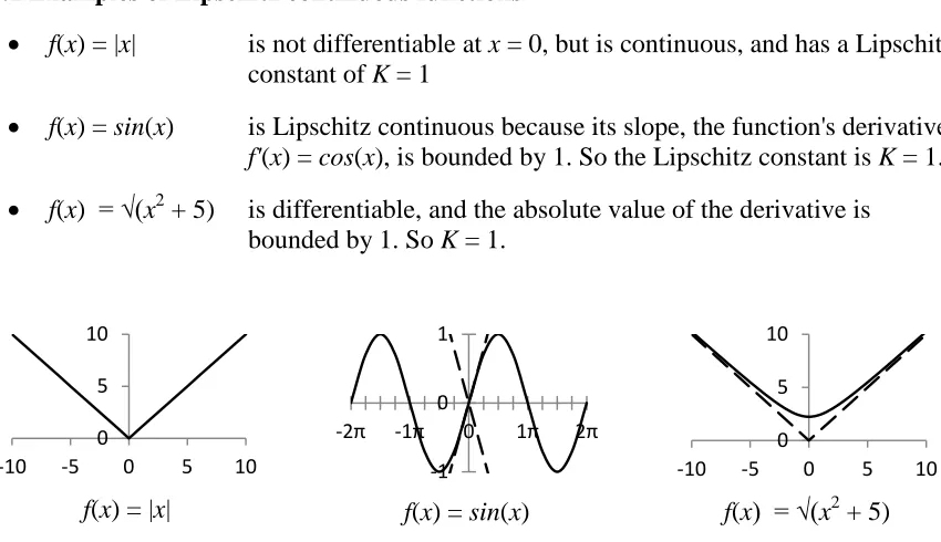
• f(x) = |x| is not differentiable at x = 0, but is continuous, and has a Lipschitz constant of K = 1
• f(x) = sin(x) is Lipschitz continuous because its slope, the function's derivative f'(x) = cos(x), is bounded by 1. So the Lipschitz constant is K = 1.
• f(x) = √(x2 + 5) is differentiable, and the absolute value of the derivative is bounded by 1. So K = 1.
f(x) = |x| f(x) = sin(x) f(x) = √(x2 + 5) Figure 2.2 - Functions that are Lipschitz continuous over the real domain
2.1.2 Examples of Continuous Functions that are not Lipschitz Continuous
• f(x) = √(x) is continuous, but not Lipschitz continuous, because the slope becomes infinitely steep a x→ 0.
• f(x) = ex is also continuous, but the slope becomes infinitely steep as x→ +∞.
• f(x) = x2 is continuous along the domain of all real numbers, but is not Lipschitz continuous, because the slope becomes infinity steep as x→ ±∞.
f(x) = √(x) f(x) = ex f(x) = x2 Figure 2.3 - Functions that are not Lipschitz continuous over the real domain
0 5 10
-10 -5 0 5 10 -1
0 1
-2π -1π 0 1π 2π 0
5 10
-10 -5 0 5 10
0 1 2 3 4 5
-5 -4 -3 -2 -1 0 1 2 3 4 5
0 1 2 3 4 5
-5 -4 -3 -2 -1 0 1 2 3 4 5 0
1 2 3 4 5
2.2 Lipschitz Optimization in One Dimension
Lipschitz optimization requires the knowledge of the Lipschitz constant K. Finding the true Lipschitz constant is as hard as solving the optimization problem itself [9]. The Lipschitz optimization algorithm was developed independently by Piyawskii [10] and
Shubert [11]. It is based on the assumption that the Lipschitz constant K is known. Shubert's algorithm is described here, with a brief overview, followed by detailed steps and an
illustrative example.
Figure 2.4 - First Iteration of Lipschitz Optimization with the Objective Function Estimate, B, shown for the Interval [a, b]
The Shubert algorithm finds the intersection point B of the lines with slopes of -K and +K, originating at the start and end points of the interval respectively, as shown in Figure 2.4 above. It assumes that this intersection point is a lower bound of the objective function. This assumption is true as long as the estimated Lipschitz constant K used is not less than the true Lipschitz constant. Then the algorithm evaluates the objective function at this
intersection point (X, B) and divides the interval into two sub intervals, and determines the objective function estimate, B, for each new sub interval. Then the interval with the lowest B value is further divided. The algorithm stops when the estimated objective function value, B, is within a specified tolerance, E, of the true objective function value, f, at any point. The algorithm steps below and the example given illustrate how the algorithm works.
0 0
f(
x)
x B
X +K -K
(a, f(a))
2.2.1 Algorithm Steps
First, define B(a, b) (Equation 2.1) as the estimate of the best objective function value contained in interval [a, b]. Also define X(a, b) (Equation 2.2) as the x value at the estimate for the best objective function value contained in interval [a, b].
B(a, b, f, K) = (f(a) + f(b))/2 - K∙(b - a)/2 ( 2.1) X(a, b, f, K) = (a + b)/2 + (f(a) - f(b))/(2K) ( 2.2)
Initialize
1. Evaluate the function at the bounds, f(a) and f(b). Update fmin = min(f(a), f(b))
2. Calculate B for the entire domain interval [a, b] (Equation 2.1). 3. Add this interval to a list of intervals L.
Iterate
1. Remove the interval from the list L with the least B value. 2. Evaluate the objective function at point X (Equation 2.2).
Update fmin = min(fmin, f(X)).
3. Split this interval at point X to yield two intervals [a,X] and [X,b] 4. Calculate B for each new interval.
5. Add each new interval to the list of intervals L.
6. Stop when the difference between the best objective function value fmin, and the
minimum B value, are within a predefined tolerance E (stop when fmin - Bmin < E).
2.2.2 One Dimensional Example
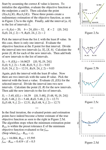
1. Start by assuming the correct K value is known. To initialize the algorithm, evaluate the objective function at the endpoints a and b. Then calculate the point
(X(a,b,f,K), B(a,b,f,K)). These three points create a rudimentary estimation of the objective function, as seen in Figure 2.5a to the right. Finally, add the interval [a, b] to the list of intervals L.
a = 0, f(a) = 20, b = 24, f(b) = 32, K = 2 {[0, 24]}
X0(0, 24, f, 2) = 9, B0(0, 24, f, 2) = 2 Figure 2.5a
2. Pick the interval from the list L with the least B value. In this case, there is only one interval. Evaluate the
objective function at the X point for that interval. Divide the interval into two intervals [a, X], [X, b]. Calculate the point (X, B) for each of the new intervals. Then add both of new intervals to the list of intervals.
X0 = 9, f(X0) = 16.0625 {[0, 9], [9, 24]}
X1(0, 9, f, 2) = 5.48, B1(0, 9, f, 2) = 9.03
X2(9, 24, f, 2) = 12.51, B2(9, 24, f, 2) = 9.03 Figure 2.5b
3. Again, pick the interval with the least B value. Now there are two intervals with the same B value. Pick the interval with the least a value. Evaluate (X, f(X)) for the selected interval. Divide the interval into two new
intervals. Calculate the point (X, B) for the new intervals. Then add the new intervals to the list of intervals.
X1 = 5.48, f(X1) = 16.39 {[0, 5.48], [5.48, 9], [9, 24]}
X3(0, 5.48, f, 2) = 5.48, B3(0, 5.48, f, 2) = 12.71
X4(5.48, 9, f, 2) = 12.51, B4(5.48, 9, f, 2) = 12.71 Figure 2.5c
… …
4. In the final iteration, the evaluated points and estimation points have indeed become a better estimate of the true objective function as seen to the right in Figure 2.5d. The algorithm stops when the minimum estimation point Bmin is within the preset tolerance E of the minimum
objective function evaluated so far fmin.
(Stop when fmin - Bmin < ε).
fmin = 16.004, Bmin = 15.595
fmin - Bmin = 0.419 < E = 0.5 Figure 2.5d
Figure 2.5 - One Dimensional Example of Lipschitz Optimization
0 2 4 6 8 10 12 14 16 18 20 22 24 26 28 30 32
0 2 4 6 8 10 12 14 16 18 20 22 24
f( x) x 0 2 4 6 8 10 12 14 16 18 20 22 24 26 28 30 32
0 2 4 6 8 10 12 14 16 18 20 22 24
f( x) x 0 2 4 6 8 10 12 14 16 18 20 22 24 26 28 30 32
0 2 4 6 8 10 12 14 16 18 20 22 24
f( x) x 0 2 4 6 8 10 12 14 16 18 20 22 24 26 28 30 32
0 2 4 6 8 10 12 14 16 18 20 22 24
f(
x)
x B0(a,b,f,K) X
0(a,b,f,K)
+K -K
(b, f(b))
(a, f(a))
(X0, f(X0))
(X1, B1) (X2, B2)
fmin
2.2.3 Disadvantages of Lipschitz Optimization Lipschitz optimization has two main disadvantages:
1. Initializing the algorithm requires the storage and evaluation of the objective function at the corners of the search domain, which requires 2N function evaluations in the first iteration, where N is the number of dimensions. This many function evaluations makes the initialization very time consuming in high dimensional problems.
Furthermore, for some problems, a single evaluation of the objective function takes a very long time to evaluate. This is especially true if the objective function uses iterative methods or simulations.
2. In many applications, the Lipschitz constant is unknown. Since finding the correct Lipschitz constant is as difficult as solving the optimization problem itself [9], estimates of the Lipschitz constant are often used. However, an incorrect estimate of the Lipschitz constant may lead to extremely slow convergence [12].
2.3 DIRECT Algorithm in One Dimension
The DIRECT algorithm was introduced by Jones, Perttunen, and Stuckman in their paper "Lipschitzian Optimization without the Lipschitz Constant" [1] specifically to overcome the shortcomings of Lipschitz optimization mentioned previously. This section describes the dimensional DIRECT algorithm, and how it differs from the
one-dimensional Lipschitz optimization. 2.3.1 Division in One Dimension
distances of one third of the interval length, ±ℓ/3. These sample points will be the centers for new sub intervals that are one third of the size of the parent interval, as shown below in Figure 2.6.
Lipschitz Optimization DIRECT Algorithm
Figure 2.6 - Comparison of Lipschitz and DIRECT Divisions
As shown in Figure 2.6, one of the main differences between the DIRECT algorithm and Lipschitz optimization is that DIRECT divides the specified interval into three
2.3.2 Potentially Optimum Intervals
When choosing the interval to further divide, the DIRECT algorithm does not simply pick the interval with the most optimal function evaluation. The DIRECT method chooses multiple "potentially optimal" intervals each iteration based on both the objective function value and the size of the interval. This section will first describe and illustrate the selection process, and then afterward give the formal definition of "potentially optimal intervals."
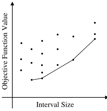
To illustrate how the DIRECT algorithm identifies potentially optimal intervals, first the intervals are plotted with the size (in this case the interval length) along the x-axis, and the objective function value is plotted along the y-axis. Then by examining this graph, all of the intervals (represented by points) along the lower right of the convex hull of these data points are chosen as potentially optimal, as shown in Figure 2.7 below.
Figure 2.7 - Graphical interpretation of "potentially optimal" interval selection, with intervals represented as points, and the "potentially optimal" intervals along the delineated convex hull
O
bj
ec
ti
ve
F
unc
ti
on V
al
u
e
Formally stated, suppose that the initial interval is divided into m sub intervals [ai, bi]
with midpoints ci, for i = 1, 2, …, m. Define fias the objective function value evaluated at
the midpoint of interval i, so that fi = f(ci), and define rias the distance from the center point
ci of the intervalto one of the end points (ai or bi) of interval i,which is the length of interval
divided by 2, so that ri = (bi - ai)/2 (ri is called the radius or the size of the interval). The
interval j is said to be "potentially optimal" if there exists some rate-of-change constant K' > 0 such that:
fj - K'∙dj≥ fi - K'∙ri, for all i = 1, 2, …, m ( 2.3)
Again, this formal statement simply makes sure that the potentially optimal intervals are on the lower right convex hull of the objective function value vs. interval size graph.
Here are some generalizations about selecting the potentially optimal intervals as described so far:
1. If all of the intervals are the same size at a given iteration, the DIRECT algorithm will pick the interval(s) with the best objective function value.
2. If there are different interval sizes at a given iteration, the DIRECT algorithm will always pick at least the interval(s) with the best objective function value overall, as well as the interval(s) that have the best objective function value among the intervals with the longest length.
2.3.2.1 Comparison of Interval Selection Methods for Lipschitz Optimization and the DIRECT Algorithm
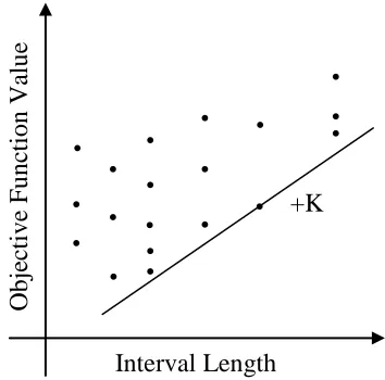
The original DIRECT paper [1] shows that Lipschitz optimization implicitly does this same kind of "potentially optimal interval" selection, by positioning a line with a fixed slope of the Lipschitz constant, K, below all of the data points, then shifting this line upwards until it touches one of the points. The algorithm then divides the interval represented by this point. This is illustrated below in Figure 2.8. The similarity in the two algorithms for one
dimension is paraphrased in the original DIRECT paper [1] as follows: "The one dimensional DIRECT algorithm is essentially Shubert's algorithm modified to use center-point sampling and to sample all potentially optimal intervals during an iteration."
Indeed, some of the main characteristics of Lipschitz optimization—the recursive division, and the incorporation of global and local search—are retained in the DIRECT method, even though many other properties of the algorithm have changed.
Figure 2.8 - Graphical interpretation of Lipschitz interval selection, with the Lipschitz constant, K, represented as a line, and the selected interval as a point along this line
O
b
jec
ti
ve
F
unc
ti
on V
al
u
e
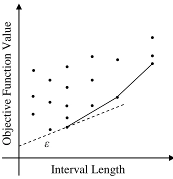
2.3.3 ε Parameter
A purely local search would only divide the intervals with the best objective function value. A purely global search would divide only the longest intervals until none of that size group is left, and then continue to divide the next size group until none of that size group is left. The global approach would be very similar to a uniform division of the search space. The DIRECT algorithm tries to balance local and global searching by dividing intervals of various size groups in the same iteration.
Figure 2.9 - Graphical interpretation of DIRECT interval selection with ε Parameter illustrated as a slope and the "potentially optimal" intervals delineated along the modified
convex hull
The introduction of the ε parameter modifies the previous formal definition of potentially optimal intervals, by adding another condition. In addition to the definitions given above, further define fmin as the minimum objective function value evaluated so far, and
define ε as a positive constant. The interval j is said to be "potentially optimal" if there exists some rate-of-change constant K' > 0 such that:
fj - K'∙rj≥ fi - K'∙ri, for all i = 1, 2, …, m ( 2.3)
fj - K'∙rj≥ fmin - ε∙|fmin| ( 2.4)
2.3.4 Algorithm Steps
First, a discussion of how to store the rectangles (or intervals in this case) will be given. Then the steps will be given for the one-dimensional DIRECT algorithm, followed by an example in Section 2.3.5.
O
bj
ec
ti
ve
F
unc
ti
on V
al
u
e
Interval Length ε
2.3.4.1 Rectangle Storage
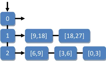
The process of determining the potentially optimal rectangles requires a specialized data structure to be algorithmically efficient. All of the rectangles must be organized by size first, then by objective function value. He et al. [7] describes a data structure to store the potentially optimal rectangles. For this research, the rectangles are organized as a list of lists. The primary list contains the secondary lists and it is indexed by rectangle size. More
specifically, the number of times, T, the rectangle has been divided can be used as an integer index for the secondary lists, since T is directly proportional to the rectangle size. The secondary lists (referred to as size groups) contain the rectangles of the same size and are sorted by objective function value evaluated at the midpoint. This type of data structure is shown in Figure 2.10 below.
Figure 2.10 - Rectangle Storage for Potentially Optimal Determination
Now, only the rectangles with the best objective function values per size group need to be checked against Conditions 2.3 and 2.4 for being potentially optimal. However, it is possible for multiple rectangles of the same size to have the same objective function value. Therefore, all of the rectangles in a size group with the best objective function value must be checked. Since, the secondary lists are sorted, all of the rectangles with the best objective function value will be at the front of the list.
0
1
2
[9,18] [18,27]
2.3.4.2 DIRECT One Dimensional Steps
Given a data structure, similar to the one shown in Figure 2.10, to store the intervals (called SizeRects or "the list of all rectangles"), here are the steps for the one-dimensional DIRECT algorithm.
Initialize
1. Sample the midpoint of the entire search space. 2. Add the initial interval to SizeRects.
Iterate
1. Determine the Set P of all potentially optimal intervals in SizeRects. Remove Set P from SizeRects.
2. For each interval I in Set P:
a. Evaluate points ±1/3 the length of interval I from the midpoint of I Increment the function counter m by 2.
b. Divide I into thirds, such that the points evaluated previously are now the centers of these new intervals.
c. Add the new intervals into a temporary Set R.
3. Clear Set P. Add the Set R of new intervals to SizeRects. Clear Set R. Increment the iteration counter i by 1.
4. Stop when the evaluation counter m is greater than the maximum number of function evaluations mmax, or when the iteration count is greater than the maximum number of
iterations imax (Stop when i > imaxor m > mmax).
2.3.5 One Dimensional Example
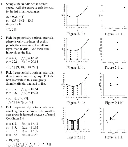
The following example shows the first four iterations of the one-dimensional
number times the interval has been divided. Since the graph has a log scale, the straight lines on the convex hull are not accurate, but serve as illustrations.
1. Sample the middle of the search
space. Add the entire search interval to the list of all rectangles.
a0 = 0, b0 = 27
c0 = (27 - 0)/2 = 13.5
f(c0) = 17.89
{[0, 27]}
Figure 2.11a Figure 2.11b
2. Pick the potentially optimal intervals, (there is only one interval at this point), then sample to the left and right, then divide. Add these sub intervals to the list.
c1 = 4.5, f(c1) = 16.78
c2 = 22.5, f(c2) = 29.14
{[0, 9], [9, 18], [18, 27]} Figure 2.11c Figure 2.11d
3. Pick the potentially optimal intervals, there is only one size group. Pick the best intervals in this size group. Sample, divide, and add to list.
c3 = 1.5, f(c3) = 18.64
c4 = 7.5, f(c4) = 16.02
{[9, 18], [18, 27]}
{[6, 9], [3, 6], [0, 3]} Figure 2.11e Figure 2.11f
4. Pick the potentially optimal intervals, checking the conditions. The smallest size group is ignored because of ε and Condition 2.4.
c5 = 6.5, f(c5) = 16.14 c6 = 8.5, f(c6) = 16.02 c7 = 10.5, f(c7) = 16.39 c8 = 16.5, f(c8) = 20.52
{[18, 27]}
{[9,12],[3,6],[12,15],[0,3],[15,18]} {[8, 9], [7, 8], [6, 7]}
Figure 2.11g Figure 2.11h
Figure 2.11 - One Dimensional Example of DIRECT Optimization
0 4 8 12 16 20 24 28 32 36 40
0 3 6 9 12 15 18 21 24 27
f( x) x 0 5 10 15 20
0.019 0.056 0.167 0.500
f( x) Size 0 4 8 12 16 20 24 28 32 36 40
0 3 6 9 12 15 18 21 24 27
f( x) x 0 5 10 15 20 25 30 35
0.019 0.056 0.167 0.500
f( x) Size 0 4 8 12 16 20 24 28 32 36 40
0 3 6 9 12 15 18 21 24 27
f( x) x 0 5 10 15 20 25 30 35
0.019 0.056 0.167 0.500
f( x) Size 0 4 8 12 16 20 24 28 32 36 40
0 3 6 9 12 15 18 21 24 27
f( x) x 0 5 10 15 20 25 30 35
0.019 0.056 0.167 0.500
f(
x)
2.4 DIRECT Algorithm in Two or More Dimensions
The main difference between the one-dimensional DIRECT algorithm and the multi-dimensional DIRECT algorithm is how the potentially optimal hyperrectangles are divided. There are two other small differences. One difference is that, in the initialization of the algorithm, the search space is normalized to a unit hypercube. The second difference is the definition of rectangle size. These details are explained in this section.
2.4.1 Normalization to a Unit Hypercube
Normalization is performed to convert all of the variable ranges from their original upper and lower bounds to a range between 0 and 1. Conversion back to the original values only needs to be performed when calling the objective function. Normalizing the variables means that the side lengths of each rectangle will all be multiples of 1/3. This step is supposed to make the division calculations simpler.
2.4.2 Division in Two or More Dimensions 2.4.2.1 Division of a Hypercube
The original DIRECT algorithm divides the hypercube into thirds along every dimension around the center point. It also divides the hypercube along all of the dimensions in a specific order in an attempt to avoid premature, local convergence.
First, the algorithm samples the objective function at points around the center point, plus and minus one-third of the cube's side length in every dimension. Formally stated, it samples points c ± δui for all i = 1, 2, …, n, where c is the center point of the hypercube, δ is
one-third the side length of the hypercube, n is the number of dimensions, and ui is a unit
Now with all of these samples evaluated, DIRECT sorts the dimensions based on the best out of the two samples per dimension. Then, the algorithm divides the hypercube in thirds along the dimension with the best objective function value first, and then it recursively divides the center rectangle along the subsequent dimensions in order of their best function value. This means that the dimension with the best objective function value will have the largest rectangles. The divisions are performed in this order to allow the area with the best objective function value to be searched more. If the dimensions were divided in the reverse order, the dimension with the best objective value would have the smallest rectangle, and this could lead to premature convergence at a local optimum. Figure 2.12 shows a hypercube sampled and divided in two dimensions. The objective function values are shown above the sample point.
Figure 2.12 - DIRECT sampling and division in two dimensions with the objective function value shown above each point
2.4.2.2 Division of a Hyperrectangle
Once the initial hypercube is divided, there will be many hyperrectangles as well as smaller hypercubes. The hyperrectangles are divided in a similar manor as the hypercube, except that only the longest sides of the rectangle are sampled, sorted, and divided.
21.42 21.42
34.91
32.66 20.28
18.03
21.42 34.91
32.66 20.28
2.4.2.3 Division Steps
The steps for dividing potentially optimal hyperrectangles are described below. These include the hypercube as a special case of hyperrectangle.
1. Identify the set I of dimensions for the potentially optimal hyperrectangle with the longest side length. Define δ as one-third of the longest side length.
2. Evaluate the objective function at the points c ± δui for each dimension i in the set I,
where c is the center point of the potentially optimal hyperrectangle and ui is the unit
vector in the ith dimension.
3. Sort the dimensions in set I by the lowest objective function value vi for each
dimension, from the least to the greatest. vi = min{f(c + δui), f(c - δui)}
4. Divide the potentially optimal rectangle along each of the dimensions in set I in the sorted order from the least function value vi to the greatest, such that the dimension
with the least objective function value has the largest sub rectangles. 2.4.3 Rectangle Size
In the one-dimensional DIRECT, the interval is essentially the one-dimensional rectangle, and its size is measured by the distance from the center point to the end point of the interval i, which is the same as the length of the interval divided by 2, ri = (bi - ai)/2.
2.4.4 Algorithm Steps
The algorithm steps have not significantly changed from the one dimension algorithm except for the addition of normalization in the initialization, and a more complicated division strategy. The procedure for determining potentially optimal rectangles is still the same, only with a slightly modified definition of rectangle size. The objective function value vs.
rectangle size plot and lower right convex hull strategy still holds. Below are the steps for the multi-dimensional DIRECT algorithm, given a data structure for organizing rectangles called SizeRects as described earlier in Section 2.3.4.1 .
Initialize
1. Normalize all variables to the unit hypercube. 2. Sample the midpoint of the entire search space. 3. Add the initial rectangle to SizeRects
Iterate
1. Determine the Set P of all potentially optimal intervals in SizeRects. Remove Set P from SizeRects.
2. For each Rectangle R in Set P:
a. Sample and evaluate points c ± δui for all dimensions i = 1, 2, … n
Increment the function counter mby 2∙n.
b. Divide Rectangle R into thirds along every dimension, such that the points evaluated previously are now the centers of these new rectangles.
c. Add the new rectangles into a temporary Set T 3. Clear Set P. Add the Set T of new rectangles to SizeRects.
Increment the iteration counter i by 1.
4. Stop when the evaluation counter m is greater than the maximum number of function
evaluations mmax, or when the iteration count is greater than the maximum number of
2.4.5 Two Dimensional Example
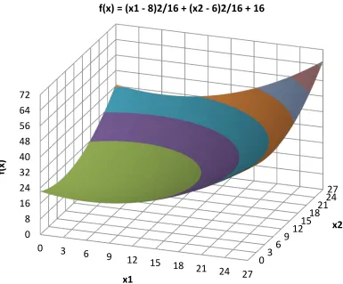
This two dimensional example shows the first three iterations of the DIRECT algorithm to optimize the objective function f(x) = (x1 - 8)2/16 + (x2 - 6)2/16 + 16 in the
domain 0 ≤ xi≤ 27 for i∈ {1,2}. This function is quadratic, and is graphed in Figure 2.13.
When displaying the SizeRects structure, the rectangles are represented by their center point. Also, the grayed rectangles indicate that they will be picked as potentially optimal in the next iteration.
Figure 2.13 - Objective Function for Two Dimensional DIRECT Example
03
69
1215 1821
2427
0 8 16 24 32 40 48 56 64 72
0 3 6
9 12 15 18 21
24 27
x2
f(x
)
x1
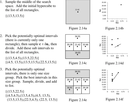
1. Sample the middle of the search space. Add the initial hypercube to the list of all rectangles.
{(13.5,13.5)}
Figure 2.14a Figure 2.14b 2. Pick the potentially optimal intervals
(there is currently only one
rectangle), then sample c ± δui, then
divide. Add these sub intervals to the list of all rectangles.
{(13.5,4.5),(13.5,22.5)}
{(4.5, 13.5),(13.5,13.5),(22.5,13.5)} Figure 2.14c Figure 2.14d 3. Pick the potentially optimal
intervals, there is only one size group. Pick the best intervals in this size group. Sample, divide, and add to list.
{(13.5,22.5)}
{(4.5,4.5),(13.5,4.5),(4.5, 13.5),
(13.5,13.5),(22.5,4.5), (22.5, 13.5)} Figure 2.14e Figure 2.14f Figure 2.14 - Two Dimensional Example of DIRECT Optimization
2.5 Changes to the DIRECT Algorithm from Prior Research
There have been many changes to the DIRECT method reported in the literature to improve efficiency or to adapt DIRECT to a specific application. Modifications to the DIRECT algorithm relevant to this research are discussed here.
2.5.1 Aggressive DIRECT
The original DIRECT algorithm does not divide the same number of rectangles every iteration. Usually the number of rectangles considered "potentially optimal" grows each
0.00 5.00 10.00 15.00 20.00 25.00
0 0.25 0.5 0.75 1
f( x) Size 0.00 5.00 10.00 15.00 20.00 25.00 30.00 35.00 40.00
0 0.25 0.5 0.75 1
f( x) Size 0.00 5.00 10.00 15.00 20.00 25.00 30.00 35.00 40.00
0 0.25 0.5 0.75 1
iteration. This makes DIRECT difficult to scale for parallel performance. The Aggressive DIRECT algorithm (Aggressive DIRECT) was introduced by Baker et al. [13] specifically to improve parallel performance. It does this by changing the definition of potentially optimal. Instead of using the convex hull strategy, Aggressive DIRECT divides all of the rectangles that have the best objective function value for each size group, as shown below in Figure 2.15. The number of rectangles divided still grows with each iteration, but the number of rectangles (and thus the number of function evaluations) is very large except in the early iterations. Therefore, the Aggressive DIRECT algorithm becomes almost embarrassingly parallel, and can yield good parallel performance scalability.
Figure 2.15 - Graphical interpretation of the rectangle selection using Aggressive DIRECT with most optimal rectangle of each size group selected and delineated in the plot
2.5.2 Dividing Only One Dimension
In a later article [3], Jones suggested, instead of the more complicated division strategy in the original DIRECT algorithm, to simply divide the hyperrectangle along only
O
bj
ec
ti
ve
F
unc
ti
on V
al
u
e
one of the longest sides. Apparently, there is little to no improvement gained by recursively dividing all of the dimensions and using the dimension sorting procedure described in Section 2.4.2.3. Furthermore, dividing only one dimension at a time saves function
evaluations and time used in sorting the dimensions. In the words of Jones: "Experience has since shown, however, that the robustness benefit is small and that trisecting on a single long side (as here) accelerates convergence in higher dimensions."
Jones also gives a procedure for breaking ties among the rectangles longer sides. He suggests keeping a counter ti of how often each dimension i has been divided in the entire
search (the counter is for the division of any rectangle along dimension i). To decide
between the longer sides of the hyperrectangle choose the side with the lowest division count ti, and if two of the long sides have the same division count, then choose the side with the
lowest dimension index i.
2.5.3 Generalized Definition of Rectangle Side Length and Radius
A generalized version of the rectangle side length and the rectangle radius (distance from the center point one of the vertices) is first described in the Jones article [3]. It is further detailed in a thesis by Gablonsky [2]. The generalized definitions for rectangle side length and radius are described below, as well as how the radius definition affects the selection of "potentially optimal" rectangles.
2.5.3.1 Side Length
distance (the radius) can be generalized. First, define T as the total number of times a
particular rectangle has been trisected, and define N as the total number of dimensions. Then define the level as k = ⌊T / N⌋ and the stage as j = mod(T, N). It can be shown that
T = k·N + j. Before explaining the meaning of the level k and stage j, it is important to note that for any given rectangle used in the DIRECT method, there are only two side lengths, a longer side length and a shorter side length. This is because the DIRECT method always divides one of the longer sides. The longer side length can be represented as ℓ = 3-k, and the shorter side length will be ℓs = 3-(k + 1). Conceptually, the level, k, is the number of times the
longest side has been trisected, and the stage, j, is a count of the shorter sides for that particular rectangle.
2.5.3.2 Radius
The radius of the rectangle can also be abstracted. Using simple algebra, the radius r (Equation 2.8) is determined from the level k (Equation 2.5) and the stage j (Equation 2.6) as shown below:
k = ⌊T / N⌋ ( 2.5)
j = mod(T, N) ( 2.6)
T = k·N + j ( 2.7)
𝑟= 3−𝑘2 �𝑗9+ 𝑁 − 𝑗�0.5 = 3−𝑘2 �𝑁 −8𝑗9 ( 2.8)
2.5.3.3 Rectangle Size Definition
In the original DIRECT algorithm, the rectangle size is synonymous with the rectangle radius r (i.e. the center-to-vertex distance), which directly corresponds to the number of times the rectangle has been divided T. However, in later research by Gablonsky [2], this size definition was changed to be the level k of the rectangle. The level of the rectangle was defined in the previous section to be the number of times the longest side of the rectangle has been divided k = ⌊T / N⌋ (Equation 2.5). The definition of rectangle size was changed in order to group more rectangles in a size group, so that there would be fewer potentially optimal rectangles chosen per iteration. Gablonsky took the opposite approach to the Aggressive DIRECT algorithm, in that he was trying to reduce the number of potentially optimal rectangles per iteration. The change in size definition was found to reduce the total number of function evaluations needed to find the optimal solution for certain test functions. However, it did increase the number of iterations.
2.5.4 Only One Minimum Rectangle per Size Group
2.5.5 Integer Variables
In the same article where Jones suggests dividing only one dimension and generalizes the definition of rectangle radius and side length [3], he also modified the algorithm to handle integers and inequality constraints. Jones mentions two minor changes that have to be made to make DIRECT work with integers: one is in the way the midpoint of the rectangle is defined, and the second is in the trisect routine.
2.5.5.1 Integer Midpoint
Redefining the midpoint is trivial. Jones defines it as the floor of algebraic average for each dimension. For example, for the interval [1, 8], the integer midpoint cannot be 4.5, which is (b - a)/2 as previously defined. So the integer midpoint is defined as ⌊(b - a)/2⌋ for the interval [a, b] (in this example 4). Therefore, the integer midpoint for multiple
dimensions is the floor of algebraic average for the interval of each dimension. 2.5.5.2 Trisecting Integers
2.5.5.3 Resolving Complications
Using integer variables yields three more complications, which Jones addresses in the article: 1. Because the midpoint of the integer dimension will not truly be at the geometric
center, the center-to-vertex distance is not the same from the midpoint to all of the vertices. This is resolved by ignoring the actual center-to-vertex distance, and instead using the radius formula (Equation 2.8) given above, which is based solely on the number of dimensions and the number of times the rectangle has been divided. 2. The floored integer division procedure yields side lengths that are not precisely in the
ℓ = 3-k format. This means that sides that have been divided the same number of times will not necessarily be the same length. The side length is mainly important in determining which sides are the longest and choosing the dimension to divide. This problem is solved by relaxing the definition of longest sides to mean those sides that have been divided the least number of times. Furthermore, if a side has a length of 0, meaning it only has one integer within that side's range [a, a], it will not be further divided.
3. Finally, if all of the variables are integers, then a rectangle could be reduced to a single point. In this case, the rectangle will be ignored from the "potentially optimal" selection process and will not be divided anymore.
2.5.6 Adaptive ε Parameter
a local optimum, and the algorithm will change the ε parameter to a higher value to induce a more global search. If there is no improvement, with the higher ε value, then the algorithm switches back to a more local search with ε = 0.
Chapter 3 The DIRECT Algorithm for the Generic Variable Type
The motivation for an abstract variable type is to be able to use other discrete variable types with the DIRECT method, specifically to use nodes in a water distribution system (WDS), which are essentially graph nodes. To be able to use DIRECT with graph nodes, more abstraction and generalization is needed, in the same manner that Jones abstracted the DIRECT method for integer variables, and mixed real and integer problems. This chapter details the generalizations that are made.
3.1 Generalized Variable Type
This section develops an interface for the generic variable type. An interface is used in computer programming as a class with abstract functions that are defined by the
implementing classes, like a header file in C or C++. The interface is a template that needs the specific implementations to be further defined by the child objects. Such an interface is given in Table 3.1.
As Jones noted when changing the DIRECT method to handle integer types, the two main considerations are how to handle the division and how to select a midpoint of the variable range. These will be the first two generalizations discussed in this section.
It is important to note that a side of the rectangle is a dimension of the rectangle, and both represent a variable being search by the DIRECT algorithm. Therefore the words variable, side, and dimension are essentially synonymous in this discussion.
Table 3.1 - General Variable Interface Interface Variable
1: 2: 3: 4: 5: 6: 7: 8: 9: 10: 11:
interface Variable properties
int divcount end properties
methods
Variable[] trisect()
float midpoint() boolean issingular() Variable copy() end methods
end interface
3.1.1 Division
Each time a variable is divided, the divcount counter should be incremented in each of its child variables. That way this counter is an accurate count of the number of times a variable has been divided.
Table 3.2 - Possible Division Procedures for Various Variable Types Variable Type Possible Division Procedures
Real A real variable range [a, b] can be divided into three child
variables [a, a +Δ], [a +Δ, b -Δ], [b -Δ, b], where Δ = (b - a)/3 Integer An integer variable range [a, b] can be divided into three child
variables [a, a +Δ - 1], [a +Δ, b -Δ], [b -Δ + 1, b], where Δ = ⌊(b - a + 1)/3⌋ (see Section 2.5.5)
Discrete Set A discrete set of sorted integer or real numbers can be divided into subsets where each subset has approximately the same number of members per subset
For example, {1, 2, 4, 8, 16, 32, 64} can be divided into three subsets {1, 2}, {4, 8, 16}, {32, 64}.
Binary A binary variable can be trisected, so that the third child is NULL. {0, 1} → {0}, {1}, NULL
Cartesian Points A set of Cartesian points can be divided into three subsets based on either the x-coordinate or the y-coordinate, or it can alternate between the dimension it divides each time the variable is divided. Graph Nodes A set of graph nodes can be partitioned based on adjacency
information, such as using recursive minimum cuts, or using clustering algorithms.
Water Distribution System (WDS) Nodes
3.1.2 Midpoint
Each Variable also has a midpoint method that returns the midpoint of the variable's range. This method returns a floating-point type, but if the variable is an integer type it can still return an integer cast as a floating point, and if the variable type is a graph node, it can return the node's index (an integer) cast as a floating point.
This midpoint method is called when the objective function value of the rectangle midpoint of the rectangle is evaluated. The objective function is responsible for casting the floating-point midpoint before use. Since the variables of a rectangle are ordered, the objective function casts and uses each floating-point midpoint number appropriately. For example, if the variable is an integer type variable, the floating-point midpoint will be cast to an integer.
3.1.3 Singularity
As Jones pointed out in [3], when dealing with integer variables, care must be taken when the size of the variable’s range reduces to below three. Specifically, if there is only one item in the variable’s range, then it should not be divided any more. The issingular method returns a boolean that is true if the variable only contains one item, and it returns false otherwise. When a variable is trisected with only two items, one of the child variables will be NULL.
3.1.4 Copy
The three child rectangles will each receive one of the new child variables respectively, as well as copies of the other variables that were not divided.
3.2 Generalized Rectangle
The rectangle interface given below in Table 3.3 standardizes the methods available and so that interaction with the various variable types is made clear.
Table 3.3 - General Rectangle Interface Interface Rectangle
1: 2: 3: 4: 5: 6: 7: 8: 9: 10: 11: 12:
interface Rectangle properties
int divcount int ndims end properties methods
Rectangle[] trisect(int n)
float[] midpoint() boolean issingular() float radius() end methods
end interface
3.2.1 Division 3.2.1.1 Trisect
3.2.2 Midpoint
The midpoint method returns the midpoint of the rectangle. This midpoint can be thought of as a "central" or representative sample of the decision space contained within the rectangle. This midpoint is not necessarily geometrically central, because some of the variable types solved for in the problem may be discrete. The method returns an array of floating-point numbers that is the midpoint of this rectangle. The array is made up of the midpoints of each of the variables that comprise this rectangle. For example, the first
element of the array will be the midpoint of the first variable in the rectangle, and the second element will be the midpoint of the second variable, etc. This midpoint is the solution that is evaluated in the objective function, and represents this rectangle when determining the potentially optimal rectangles.
3.2.3 Singularity
The rectangle is considered singular if all of its variables are singular, as previously defined in Section 3.1.3. If the rectangle is singular, it means that there is only one solution contained within the rectangle, and that the rectangle will not be considered for division any longer. However, the objective function value of the singular rectangle will still be
considered when determining the best solution found. 3.2.4 Radius
radius is the measure of rectangle size used when determining the potentially optimal rectangles. It is the x-axis in the objective function value vs. rectangle size plot. 3.3 Test Functions
In the original DIRECT paper by Jones et al. [1], there are numerous test functions given to gauge the performance of DIRECT compared to other algorithms. In the thesis by Gablonsky [2], he also used these test functions to compare his modifications to the original DIRECT algorithm. Table 3.4 below presents some of these test functions. The number of function evaluations to find the known global minimum is given for the original application of the DIRECT method, for Gablonsky's results, and for the results of this research. In this research, the version of the DIRECT algorithm used to solve these test functions divided only one dimension at a time, sorted the rectangles by the longest side (level), and only considered one of the minimum rectangles per size group as potentially optimal, unless noted otherwise.
Table 3.4 shows that the version of DIRECT used in this research was able to outperform both the original DIRECT algorithm and Gablonsky’s version of DIRECT in some cases (indicated in bold). In few cases, this version of DIRECT only outperformed the original DIRECT method, but did not outperform Gablonsky’s version. Finally, this version of DIRECT underperformed both the original DIRECT algorithm and Gablonsky’s DIRECT for the Shekel functions, which have a relatively flat objective space with many local
divide all the dimensions of a rectangle in one iteration. For most cases, dividing only one dimension at a time reduces the number of function evaluations, but not in every situation.
Table 3.4 - Function Evaluations to find Global Minimum for Test Functions Number of Function Evaluations
to find Global Minimum * DIRECT Methods
N Dims Range Global
Min
1991 Jones et al.
2001 Gablonsky
This Research
Linear 2 [0,1]2 0 475 173 171
Quadratic 2 [0,10]2 10 139 65 49
Branin 2 [-5,10]×[0,15] 0.397887 195 159 135
Shekel 5 4 [0,10]4 -10.153 155 147 183
Shekel 7 4 [0,10]4 -10.403 145 141 193
Shekel 10 4 [0,10]4 -10.536 145 139 257**
Hartman 3 3 [0,1]3 -3.863 199 111 155
Hartman 6 6 [0,1]6 -3.322 571 295 171
Goldstein Price 2 [-2,2]2 3 191 115 107
Six-hump Camel
Back 2 [-3,3]×[-2,2] -1.03163 285 191 197
Chapter 4 Leak Detection in Water Distribution Systems (WDS) using the
Dividing Rectangles (DIRECT) Search
This chapter introduces the leak detection problem in WDS (Section 4.1), describes WDS simulation and optimization (Section 4.2), and details the specific problem
representations used in this research (Section 4.3). 4.1 Introduction to Leak Detection
4.1.1 Motivation
Water distribution systems are a vital part of modern infrastructure, bringing safe clean drinking water to the public. Yet these systems are susceptible to leaks and
contaminant intrusion. High pressures, freezing water, corrosion, and aging can cause cracks in the distribution pipes. It has been estimated that anywhere between 3 and 50 percent of water is lost to leaks in a WDS: three percent in well-maintained systems, and fifty percent in aging systems and in developing countries [8]. Large leaks are usually easy to locate because they can cause significant property damage and flooding, but small leaks gradually loose water into the soil and can be difficult to locate. Leaks cause the pressure to drop in the system, which requires more pumping to maintain the required pressure. If there is negative pressure in the pipe, a leak can become a contaminant intrusion point by leaching chemicals from soil into the water.
4.1.2 Current Approaches
other field methods, such as thermal imaging and tracer gas analysis. There are also simulation-based approaches, the most common of which is called Inverse Transient
Analysis (ITA). However, ITA requires the use of induced pulses (e.g. opening and closing a fire hydrant), and then backward calculation to determine the leak location. Also, ITA is usually used for locating leaks along a straight long pipe, not in a water network.
These current methods, however, are usually expensive and time consuming. This research seeks to use measurements that can be routinely collected, such as the pressure and chlorine concentration at sensor nodes, and the flow through certain metered pipes. In some more progressive utilities, these measurements can be obtained in real time. These
measurements can carry a signature that will help identify the leak location and magnitude by using an inverse-modeling approach, potentially reducing the time and expense of leak detection.
4.2 Water Distribution Simulator
input to the water distribution simulator and it will affect the pressure, quality, and flow values, as illustrated in Figure 4.1.
Figure 4.1 - The WDS Simulator
4.2.1 Leak Representation
Leaks are modeled in EPANET as emitters, such as a sprinkler or a fire hydrant. The distinction between an emitter and a demand, is that a demand is a flow out of a node that is known and fixed at each timestep, but an emitter is a flow that depends on the pressure at that node at that time. The equation for the emitter flow is given below (Equation 4.1).
fn,t = cn·pn,tγ ( 4.1)
where n is the emitter node (i.e. leak node), t is the current timestep, γ is called the pressure exponent and is fixed at γ = 0.5, p is the pressure at node n at time t, f is the emitter flow (i.e. flow through the leak) for node n at time t, and c is the emitter coefficient for node n.
The variables in this equation when modeling leaks are the leak location (the leak node n), and the leak magnitude (the emitter coefficient cn).
• Demands • Network
Configuration
• Flows • Pressures • Chlorine WDS
Simulator
4.2.2 Inverse Modeling Approach
It is not a straightforward operation to invert complex models in EPANET to obtain the inputs, such as leak location and magnitude, from the outputted pressure, flow, and water quality values. However, this problem can be formulated as a parameter estimation problem, and an inverse modeling approach (specifically, a simulation-optimization approach) can be used to determine the leak locations and leak magnitudes. In this approach, the leak
parameters can be iteratively estimated by using the WDS simulator as the objective function that returns the simulated pressure, quality, and flow values. Then the difference (or error) between the simulated and the measured values can be calculated. By minimizing this error, a better estimation of the leak parameters is made. This is an optimization problem
minimizing the difference between the simulated and measured sensor values for pressure, quality, and flow. Figure 4.2 shows the simulated and measured values being compared to make better estimates of the leak parameters.
Figure 4.2 - The Simulation Optimization Approach • Demands
• Network Configuration
• Flows • Pressures • Chlorine WDS
Simulator
• Leaks
• Flows • Pressures • Chlorine
Simulated Measured
4.2.3 Objective Function
As previously stated, the goal of this inverse modeling approach is to find the leak parameter values (location and magnitudes) that minimize the error between the simulated values and the measured values. Since there are three different type of measurements with different units and magnitudes (for pressure [ft], quality [mg/L], and flow [gpm]), they are normalized to be incorporated into a single objective function. Equation 4.2 below gives the normalized objective function, which is minimized for this leak detection problem.
∑ ∑ �𝑝𝑛 𝑡 𝑛𝑡−𝑝𝑛𝑡0 �2
∑ ∑ �𝑝𝑛 𝑡 𝑛𝑡0 �2
+
∑ ∑ �𝑞𝑛 𝑡 𝑛𝑡−𝑞𝑛𝑡0 �2
∑ ∑ �𝑞𝑛 𝑡 𝑛𝑡0 �2
+
∑ ∑ �𝑓𝑙 𝑡 𝑙𝑡−𝑓𝑙𝑡0�2
∑ ∑ �𝑓𝑙 𝑡 𝑙𝑡0�2
( 4.2)
where p represents the pressure values, q the quality values, f the flow values, t the current timestep, n the sensor node, l the sensor link (pipe), and 0 the measured values (observed, instead of simulated).
Figure 4.3 below shows the objective function as used in this simulation-optimization approach, along with the decision variables.
Figure 4.3 - The Simulation Optimization Approach with Decision Variables and Objective Function
∑ ∑n t(pnt−pnt0)2 ∑ ∑n t(pnt0)2 +
∑ ∑n t(qnt−qnt0)2 ∑ ∑n t(qnt0)2 +
∑ ∑l t(flt−flt0)2 ∑ ∑l t(flt0)2
Objective Function (Error):
Decision Variables: {n, cn}
• Demands
• Network Configuration
• Flows
• Pressures
• Chlorine
WDS Simulator
• Leaks
?
• Flows
• Pressures