Classification of aircraft images using different architectures of radial basis function neural network : a performance comparison

ARCHITECTURES OF RADIAL BASIS FUNCTION NEURAL

NETWORK: A PERFORMANCE COMPARISON

Puteh Saad, Subariah Ibrahim and Nur Safawati Mahshos

Department of Software Engineering, Faculty of Computer Science & Information System University Technology Malaysia, 81310 Skudai, Johor, Malaysia

Tel: +607-5532344 Fax: +607-5565044

Email: I.llteh@[email protected]@gmail.com

Abstract; Four Radial Basis Network architectures are evaluated for their performance in terms

of classification accuracy and computation time. The architectures are Radial Basis Neural

Network, Goal Oriented Radial Basis Architecture, Generalized Gaussian Network, Probabilistic

Neural Network. Zernike Invariant Moment is utilized to extract a set of features from the

aircraft image. Each of the architectures is used toclassify the image feature vectors. It is found that Generalized Gaussian Neural Network Architecture portrays perfect classification of 100%

at a fastest time. Hence, the Generalized Gaussian Neural Network Architecture has a high

potential to be adopted to classify images in a real-time environment.

Keywords; Zernike Invariant Moment, Aircraft Image Classification, Radial Basis Neural

Network, Generalized Gaussian Network, Probabilistic Neural Network

1. INTRODUCTION

Currently there are numerous types of aircraft invented for a variety of uses namely; cargo for

transportation of goods, commercial for transporting passengers and military for national

defense. Their shapes and designs vary accordingly. Identification and classification of aircrafts

are needed for national security reasons and also for education purposes. For instance, cargo and

commercial aircrafts are allowed to tree-pass the country's airborne, however military aircraft

are strictly forbidden unless approved by the country's national security department. Production

of aircraft progressing rapidly thus only a few aircraft passionate individual can identify them

correctly, on the other hand majority cannot fathom the type of aircraft based on their shape.

A few works had been published on this area. Somaie et al. (2001) recognized 2-D aircraft

images using Back-Propagation(BP) algorithm. They utilized Hotelling Transform to extract a

set of features. They used 60 to 500 neurons in the hidden layer. The time taken to train the BP

algorithm escalated to 86.5 hours. The recognition performance is 95% as the hidden neuron is

i

less than 60 or more than 500 neurons at 3.4 seconds to 86.5 hours depending on the number of

hidden layer neurons. Abo-Zaid recognized samples of four types of aircraft images represented

as 2-D images using Back Propagation Algorithm (Abo-Zaid, 1996). An example of Translation

Invariant Transform (TIT) known as MT-Transform was used to obtain a set of invariant

features from image samples. He achieved 100 % classification rate, however he do not

mentioned the computation time utilized. Botha use BP and achieve 74.07% accuracy with 6

hidden neurons. He, too does not state the computation time taken (Botha, 2004). Chun et al

also use BP and achieve 85% accuracy (Chun et ai, 2001). He also does not state the

computation time taken. On the other hand Fatemi et al uses RBF and achieve 90% accuracy

(Fatemi et ai, 2003). They too disclosed the computation time utilized to classify the aircraft

images.

In our endeavour, Zemike Invariant Moment technique is chosen to extract a set of invariant

features from aircraft images due to its accuracy in terms of inter-class variances as reported in

(Puteh,2004). The resulting feature vectors are then classified into appropriate class using RBF

based architecture. Four different RBF based architectures are evaluated namely; Radial Basis

Architecture, Goal Oriented Radial Basis Architecture, Generalized Gaussian Neural Network

Architecture and Probabilistic Neural Network Architecture.

The next section of the paper explains ZMI as Feature Extraction technique. Section 3 describes

RBF to classify the aircraft image features. The paper continues with Section 4 reporting the

implementation. Section 5 discusses the results and Section 6 is the conclusion.

2. ZERNIKE MOMENT INVARIANT

Zemike Moment (Z.M) is chosen since it is invariant to rotation and insensitive to noise.

Another advantage of Z.M is the ease of image reconstruction because of its orthogonality

property (Teague, 1980). Z.M is the projection of the image function onto orthogonal basis

functions. Z.M also has a useful rotation invariance property where the magnitude of Z.M will

not change for a rotated image. Another main property of Z.M is the ease of image

reconstruction because of its orthogonality property. The major drawback of Z.M is it's

computational complexity (Mukundan,1998). This is due to the recursive computation of Radial

Polynomials. However in this study, we overcome the problem of computational complexity by

adopting a non recursive computation of Radial Polynomials. The computation is based on the

relationship between Geometric Moment Invariant and Z.M in order to derive Zemike Invariant

Moment.

The Z.M of order p with repetition q for a continuos image function!(x,y)

that vanishes outside the unit circle is as shown in Equation. I. I.

Jilid 20, Bi\. 4 (Disember 2008) Jumal Teknologi Maklumat

Z

-p+lfJ

To compute a Z.M

coordinates are map

denote Zemike Pol)

where the Zemike p,

relating Zemike and

Thus IZpql , the I

underlying image

Geometric Moment

Zoo = (lIn) ~

IZld

= (2In)

Z20 = (3In) [: IZ2212 = (3In)

I

3. RADIAL BASI:

Radial Basis Neural

output. Neurons in t

input nodes non-line

layer is also known

transformed linearly

(I965), a pattem-cla

probability to be

Theoretically, the me

Input ( " \ (

(1.2) (1.1)

Where... R = numberof

elements in input vector

.<>2 =numberof neuronsin layer 2

Jumal Teknologi Maklumat \

a~.~.

S:X I SI = numberof neuronsin layer 1

s~ )

LinearLayer

",1 =radbas (Ii ,IW:.: - P IIb,l) .' =plO·elin(LWl.J al +b:)

".1 is i th element of .' where .lWUlS. vector made of the i th row of IWL: Input RadialBasisLayer

r>.

R SI",

\...::J '­... ---'

Jilid 20, HilA (Disember 2008)

3. RADIAL BASIS NEURAL NETWORK

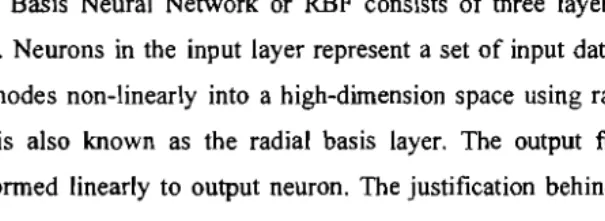
Radial Basis Neural Network or RBF consists of three layers of neurons; input, hidden and

output. Neurons in the input layer represent a set of input data. The hidden neurons transform

input nodes non-linearly into a high-dimension space using radial basis function. The hidden

layer is also known as the radial basis layer. The output from the hidden neurons is then

transformed linearly to output neuron. The justification behind this is that according to Cover

(1965), a pattern-classification problem that is transformed into a high-dimension space has a

probability to be linearly separable than in a low-dimensional space (Haykin, 1994).

Theoretically, the more neurons in the hidden layer, the more accurate will be the classification.

Figure I: Structure ofRBF neural network

Thus IZpql , the magnitude of the Z.M, can be taken as a rotation invariant feature of the

underlying image function. Rotation invariants and their corresponding expressions in

Geometric Moment are given below until the order of three:

Zoo = (1I7l:) Moo

IZld2= (2/7l:)2 (M 102+ M_OI2) Z20= (3/7l:) [2M 20+ M02) ­ Moo] IZ2i = (3/7l:)2 [(M 20 - M02)2 + 4 M112) IZ3d 2= (12/7l:)2 [(M 30 + M l2

l

l ]

IZ3312= (4/7l:)2 [(M 30- 3M I2

l

To compute a Z.M of a given image, the center of the image is taken as the origin and pixel

coordinates are mapped to the range of unit circle, i.e. x 2

+

l

denote Zernike Polynomials of order p with repetition q, and

*

.•

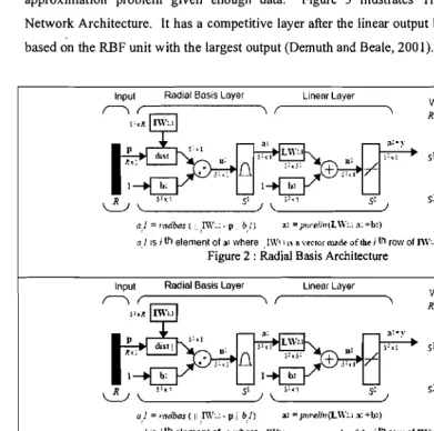
In this study four different RBF architectures are explored. In the Radial Basis Architecture

shown in Figure 2, the number of hidden nodes is equivalent to input data in the training data. In

the Goal-Oriented Radial Basis Architecture as depicted in Figure 3, the number of nodes is

-r"

i

, . '

added progressively until a desired outcome is produced. The Generalized Gaussian Network

\.::-J

Architecture as in Figure 4 consists of a set of hidden units centered at every training data. This

,,/;

unit is known as "kernels" that represent probability density functions normally of type ,",1

Gaussians. The Generalized Gaussian Network Architecture is often used for function

approximations for smooth functions, so it should be able to solve any smooth function

approximation problem given enough data. Figure 5 illustrates The Probabilistic Neural

Network Architecture. It has a competitive layer after the linear output layer that classifies data based on the RBF unit with the largest output (Demuth and Beale, 2001).

Where...

R = numberof elements in input vector

S2 =numlJer of neuronsin layer 2 SI = numberof

neuronsin layer'l LinearLayer

Radial Basis Layer

a/ = radbas l !nv:.: -p b.J) 32 =pur"lin(L \\':.1 a; +b~)

aI IS ; 1helementof .' where .rw""avecror made of the ; th row of nv:.: Figure 2 : Radial Basis Architecture Inpul

,.----.., (~---~\ r,.---~'o

'-.!:.J \.'­

Where ..

R =numberof elementsin input vector

S2 =numberof neuronsin layer 2

S'd Sl = numberof

neuronsin layer 1 LinearLayer

S-:l{l

SI ) \.

'---~ Radial Basis Layer

a,! =radbas ( !' IW:,: - P i bJ) ., =pm'elh,(l.W'.l a: +h')

aI is ; 1helementof .' where ,[WIl ... vector made of the ; th row of ny:.: Fi ure 3: Goal-Oriented Radial Basis Architecture Input

r>; r,.---~\(~---~\

.,-,. Q =no.of neurons in layer"

Q =no.of neurons in layer2

Q = no. of mpur targetpairs Q

Q ) \.

_'---

RadialBasis Layer Special linear Layer Where ..

'. ( \ R = no. of elements

in inputvector

\. lI"

Input

r>; (

a/ =radbas ( !I ,!Wi.: -p II b/) ., =purelin( nJ)

a] _r is ; th elementof .' where _; !Wi.: i•• vector wad. of the ; th row of IWl.l Figure 4: Generalized Gaussian Neural Network

5. IMPLEMENTATION, RESULTS AND DISCUSSION IMAGE ACQUISITION AND

PREPROCESSING

A k-fold cross validation technique is chosen to validate the classification results, Here image

samples are divided into k subset. Then, cross validation process repeat k times to make sure all

the subsets were trained and tested, The number of correct classification is computed using

equation (5.7). n is refers to the number data test. If testing vector is true, cr(x,y)t=l. However, if testing vector is wrong, then cr(x,y)t=O. The percentage of correct classification is given by

R ~number 01 elements in input vector Where ...

Jurnal Teknologi Maklumat

a:=y

J:xl

c

(5.7)

(5.8)

Radial Basis layer CompetiUve layer

\ ( \

Q = number 01inputttarget pairs = number 01neurons in layer ·1

K =number 01classes 01Input data =number 01neurons in layer 2

Figure 5: Probabilistic Neural Network

Input

r>. (

l~ J:'Q

'-.!!..J \

of = radbas ( ,1\\":'- P bll') a: = camp.,(L"':, a:)

a 1 is i th element 01al where 1\1,:1.: is a vectormadeof thei til row 01rwl.l

n

L

t

t = I I 4

PCC =0 100­

L

k Gk=ol k

NCC k

Jilid20, Bi\.4 (Disember 2008) 4. CROSS VALIDA TlON

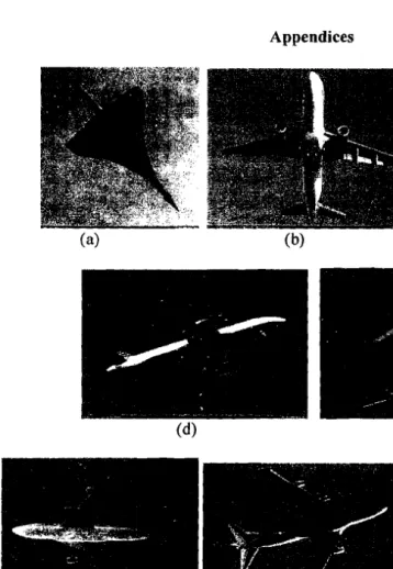
The coloured aircraft images that are downloaded from internet (www.airliners.net) are

converted into gray-level format. Noise is then removed from the image and subsequently it is

thresholded using Otsu thresholding algorithm. The resulting image is then saved using the .raw

format. Before the image file is closed, its width and height in pixels are noted since the

dimensions will become an input to the feature extraction phase. The aircraft image samples are

grouped into three categories based on their types. Category 1 represents commercial aircraft.

Category 2 represents cargo and finally Category 3 represents military. Figure 6, 7 and 8 show

the original images of each category of aircraft.

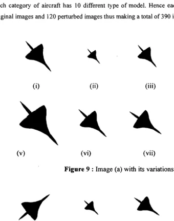
In this study, each aircraft image will become 13 images as depicted in Figure 9. For each

aircraft there are 12 images perturbed by scaling and rotation factors. The purpose of this

process is to test the invariant properties and the robustness of the feature extraction techniques

adopted. Basically, there are 4 different of scaling factors chosen namely 0.5, 0.75, 1.3 and 1.5.

For rotation factors, angles of 5°, 15°, 45° and 90° was chosen. While four images for each

aircraft are perturbed by both factors (0.5 with 5°, 0.75 with 15°, 1.3 with 45° and 1.5 with 90°).

Each category of aircraft has 10 different type of model. Hence each category consists of 10

original images and 120 perturbed images thus making a total of390 images.

(i) (ii) (iii) (iv)

Imall

(i)

(ii)

(iii) (iv)

(v)

(vi)

(vii)

(viii:

(ix)

(x)

(xi)

(xii)

(xiii'

(v) (vi) (vii)

Figure 9 : Image (a) with its variations

(ix) (x) (xii)

(xiv)

Figure 9: Image (a) with its variations (cont'.)

.Feature Extraction

.1

.~,1be

(viii)

:iJ

Tab

ZMI

0.< 0.< 0.<

45° 0.< (xiii)

90° 0.<

0.5 0.<

0.75 0.(

1.3 0.(

1.5 0.<

15"x 0.75 0.( 0.(

45"x I.J

0.(

90° x 1.5

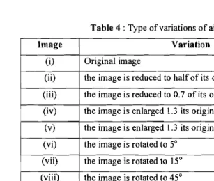
Table 4 : Type of variations of aircraft images

Image Variation

(i) Original image

(ii)

(iii)

the image is reduced to half of its original size

the image is reduced to 0.7 of its original size

I

(iv) the image is enlarged 1.3 its original size

(v) the image is enlarged 1.3 its original size

(vi) the image is rotated to 5°

(vii) the image is rotated to 15°

(viii) the image is rotated to 45°

(ix) the image is rotated to 90°

(x) the image is reduced to 0.5 and rotated to 5°

(xi) the image is reduced to 0.75 and rotated to 15°

(xii) the image is enlarged 1.3 and rotated to 45°

(xiii) the image is enlarged 1.5 and rotated to 90°

Feature Extraction

Zemike Moment features are extracted from image samples using equation (1.2). Table 5 depicts the Z.M features vectors of the same image.

Table 5 : The Z.M Feature Vector ofImage (a) and its Variants

ZMI 1 2 3 4 5 6

Original 0.00000 0.00000 0.496054 0.008847 0.020535 0.009627

5° 0.00000 0.00000 0.495574 0.008694 0.019817 0.008370 _I

15° 0.00000 0.00000 0.495431 0.008739 0.020038 0.009627

45° 0.00000 0.00000 0.497110 0.009031 0.020004 0.007078

90° 0.00000 0.00000 0.495590 0.008648 0.020367 0.006955

0.5 0.00000 0.00000 0.495738 0.008825 0.020038 0.009411

0.75 0.00000 0.00000 0.495770 0.008757 0.019979 0.009484

1.3 0.00000 0.00000 0.495620 0.008701 0.020155 0.009549

1.5 0.00000 0.00000 0.495642 0.008691 0.020191 0.009568

15° x 0.75 0.00000 0.00000 0.496542 0.008945 0.019826 0.005711

45° x 1.3 0.00000 0.00000 0.495091 0.008708 0.019019 0.006961

90° x 1.5 0.00000 0.00000 0.495644 0.008691 0.020185 0.006881

I It is observed that Z.M orders 1 and 2 have null values and order 3 is significant. Thus only rp 3

to rp 6 are utilized to train the RBF classifier.

Radial Basis Function Parameter Initialization

In order to execute RBF neural network, only one parameter need to be initialized, namely

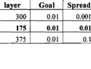
spread. Spread is to control the width of r unit in the hidden layer. According to Table 6, the best

spread value for Radial Basis Architecture is 0.01 because its sum square error (SSE) and

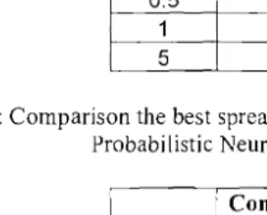
computation time is the least from other spread values. Table 7, 8 and 9 shows the comparison

for Goal Oriented Radial Basis Architecture, Generalized Regression Neural Network and

Probability Neural Network respectively. It shows that the best spread value for three architectures in the training phase is 0.001 since it produces zero error and the computation time

is the least as compared to other spread values.

Table 6: Comparison the best spread parameter value according SSE for Radial Basis Architecture

Neurons in Hidden

layer Goal Spread SSE

Computation Time

300 0.01 0.001 0.0118026 44.42

175 0.01 0.01 0.0105504 15.84

375 0.01 0.1 0.227323 150.77

Table 7: Comparison the best spread parameter value according computation time for Goal Oriented Radial Basis Architecture

Spread

Computation Time

Total Error

0.001 0.55 0

0.005 0.56 0

0.01 0.59 0

0.05 0.7 0

0.1 0.7 0

0.5 0.77 0.75

1 0.69 0

5 0.67 19.01

Table 8 : Compa

Gel

\

Table 9 : Cornpa

Cross Validation Result

In order to verify that th sub sample. Since the tc two sub samples have Three sub samples will

By using this approach, at dissimilar cycle. Figu

ktime Sub Sal I

C

2

_C

3

C

4

II

C

Figure

Table 8 : Comparison the best spread parameter value according computation time for Generalized Gaussian Neural Network Architecture

Spread

Computation Time

Total Error 0 0 11.48

0.001 0.09

c-­

0.005 0.13

0.01 0.09

0.05 0.11 15.22

0.1 0.13 36.92

0.5 0.13 42.86

1 0.06 43.8

5 0.13 38.69

Table 9 : Comparison the best spread parameter value according computation time for Probabilistie Neural Network Architecture

Spread

Computation Time

Total Error

0001 0.19 0

0.005 0.13 0.7

0.01 0.13 6.35

0.05 0.08 40.3

0.1 0.09 39.02

0.5 0.13 45.16

1 0.14 39.02

5 0.13 43.31

Cross Validation Result

In order to verify that the network has generalized well, the sample data is divided into 4 sub sample. Since the total images are 390, 2 sub samples have 98 images while another two sub samples have 97 images. The network was trained and tested for four times. Three sub samples will act as the training data and one sub sample will be the test data. By using this approach, each sample will experience being in the test set and training set at dissimilar cycle. Figure 10 illustrates the sequence of data exchanges.

ktime Sub sample 1 Sub sample 2 Sub sample 3 Sub sample 4 1

0

D

D

•

2

•

0

D

•

D

3

•

0

D

D

4

D

0

D

D

II

Figure 10: Sub sample representation for each k times

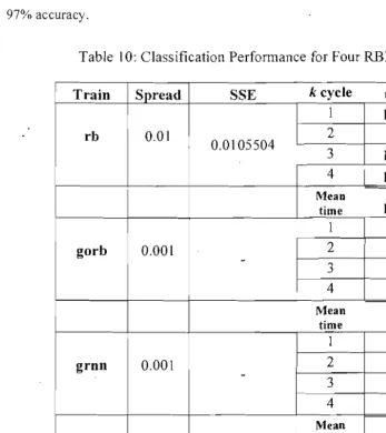
Table 10 illustrates the performance for the four REF architecture evaluated. The spread

for Radial Basis Architecture is different form others since with the value of 0.01, it

produces the least sum square error (SSE) as indicated in Table 7. It is observed that the

classification performance of Goal Oriented Radial Basis Architecture, Generalized Gaussian

Neural Network Architecture and Probabilistic Neural Network Architecture is excellent, each

of them achieve 100% accuracy. On the other hand, Radial Basis Architecture only achieves

97% accuracy.

Table 10: Classification Performance for Four REF Architectures

Network Architect:

Architecture then

Architecture has th

that, to explore tl application. Arnoi

Architecture not or

This is due to the

weights are assign:

data are inserted in

time classification;

Train Spread SSE k cycle time

NCC

rb I 0.01

0.0105504 I 2 3 15.84 15.5 16.42 98 97 98

4 _{16.14 97}

Mean

time 15.98 100

1 _{0.55 98}

gorb 0.001

-

3 _{0.56 98}

4 _{0.56 97}

Mean

time 0.61 100

I _{0.09 98}

grnn 0.001

-

3 _{0.08 98}

4 _{0.11 97}

Mean

time 0.13 100

I _{0.19 98}

pnn 0.001

- 2 3.3 97

3 0.13 98

4 _{0.09 97}

Mean

time 0.93 100

6. CONCLUSIO

In this work, v classifying aircral

that is invariance

Radial Basis Arc

Neural Network AI

architectures explo:

classification at the

repeatedly update t

training. Thus, we

to be utilized for ret

REFERENCES

Abo-Zaid, A.M (19

Radio Science Coni

19-21 Mar 1996, PI'

Botha E. C. (1994)

Legend;

In Table 10, rb represents Radial Basis Architecture 7803-1998-2. pp 13

gorb represents Goal Oriented Radial Basis Architecture

grnn represents Generalized Gaussian Neural Network Architecture

Chun, J. H. et al. (2

pnn represents Probabilistic Neural Network Architecture

neural network. Asi,

lilid 20, Bil.4 (Disern

We focus now on the computation time aspect, it is observed that the Probabilistic Neural

Network Architecture has the fastest speed, followed by Generalized Gaussian Neural Network

Architecture then Goal Oriented Radial Basis Architecture. Conversely Radial Basis

Architecture has the slowest computation time. The reason we examine the computation time is

that, to explore the feasibility of adopting the classifier for large data set in a real-time

application. Among the four architectures examined, Generalized Gaussian Neural Network

Architecture not only exhibit perfect classification but also can be performed the task the fastest.

This is due to the fact that the architecture has a function approximation capability. Here,

weights are assigned and not "trained". Existing weights will never be alternated but only new

data are inserted into weight matrices when training, thus making it a suitable candidate for real­

time classification application .

. '6. CONCLUSION

In this work, we examined the performance of four RBF based architecture in

classifying aircraft images. The images are represented using Zernike Invariant Moment

that is invariance towards rotation and scaling. The architectures that are evaluated are

Radial Basis Architecture, Goal Oriented Radial Basis Architecture, Generalized Gaussian

Neural Network Architecture and Probabilistic Neural Network Architecture. Out of the four

architectures explored, Generalized Gaussian Neural Network Architecture exhibits the perfect

classification at the fastest time. This is due to its function approximation ability that does not

repeatedly update the existing weights, only new data are inserted into weight matrices during

training. Thus, we can claim that Generalized Gaussian Neural Network Architecture is suitable

to be utilized for real-time image classification application.

REFERENCES

Abo-Zaid, A.M (I996). A simple invariant neural network for 2-D image recognition

Radio Science Conference, 1996. NRSC apos;96., Thirteenth National, ISBN: 0-7803-3656-9,

19-21 Mar 1996, pp 251 - 258.

Botha E. C. (1994). Classification of aerospace targets using superresolution ISAR images. 0­

7803-1998-2. pp 138-145.

Chun, J. H. et al. (2001). Airport pavement distress image classification using moment invariant neural network. Asian conference on Remote Sensing. (CRISP) (SISY) (AARS). Nov 2001.

I

I

Fatemi, B., Kleihorst, R., Corporaal, B.and Jonker, P. (2003) Real time face recognition on a smart camera,". Proceedings of ACIVS 2003 (Advanced Concepts for Intelligent Vision

Systems), (Gent, Belgium), 2003.

Haykin, S.(1994) "Neural Networks - A Comprehensive Foundation." Toronto, Canada:

Maxwell Macmillan.

McAulay, A., Coker, A. and Saruhan, K. (1991). Effect of noise in moment invariant neural network aircraft classification. Proceedings og the IEEE 1991 National Aerospace and

(a) Electronic Conference, NAECON. Vol. 2 pp743-749.

Mukundan, R., and Ramakrishnan, K. R. (1998). Moment Function In Image Analysis.

Farrer Road, Singapore: World Scientific Publishing.

Puteh Saad(2003), Trademark Image Classification Approaches using Neural Network and

Rough Set Theory, Ph.D. Thesis, Universiti Teknologi Malaysia.

Puteh Saad (2004), Feature Extraction of Trademark Images using Geometric Invariant Moment and Zernike Moment - A Comparison, Chiang Mai 1. Sci; 31(3):217-222.

Ii

i

Shahrul Nizam Yaakob, Puteh Saad and Abu Hassan Abdullah, Trademarks classification by

Moment Invariant and FuzzyARTMAP, Proc. of the Tenth Int. Symp. on Artificial Life and

Robotics (ARaB 10th '05), 13th - 14'h May 2005.

Shahrul Nizam Yaakob. Classification of binary insect images using Fuzzy and Gaussian ARTMAP Neural Network. MSc. Thesis. Kolej Universiti Kejuruteraan Utara Malaysia; 2006

Somaie, A. A., Badr, A. and Salah, T. (2001). Aircraft image recognition using back­

I

propagation. Radar, 2001 CIE International Conference on, Proceedings. ISBN: 0-7803-7000­

:1

7,2001.

I

I.

I

Society ofAmerica.Vol 70, No.8 pp920-930

, '

I

www.airliners.net. (10 Ogos 2007) !

Howard Demuth and Mark Beale, Neural Network Toolboxfor Use with MATLAS: User's

Guide (v. 4), The Mathworks, Inc., 2001.

Jilid 20, Bil.4 (Dise

Appendices

(a) (b) (c)

(e) (d)

(t) (g) (h)

Figure 6 : Category 1

(k) (1)

)

Figure 7 : Category 2

]ilid 20, Bi\.4 (Disember

Jilid 20, Bi\. 4 (Disember 2008) Jumal Teknologi Maklumat

(x) (y)

(z-4)

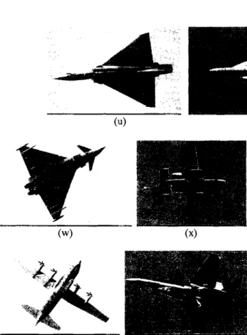
Figure 8 : Category 3

.

Table I : Category I

Image name

Aerospatiale-British Aerospace Concorde 102 Airbus A320-214 Airbus A340-313X Airbus A320-232 Airbus A380-841 Boeing 747-485 Boeing 747-4J6M Ilyushin Il-62M Boeing 747-41R Boeing 747SP-94

Table 2 : Category 2

Image Image name

k Airbus A330-243

I Boeing 737-824

m Boeing 737-...

n Dassault Falcon 10

0 McDonnell Douglas MD-II

-p DC-6A N70BF

q Boeing 747-4B5ERF

r Boeing 767-238 ER

s Boeing 747-245F SCD

t Boeing 747-422

Table 3 : Category 3

~

-APPLICAl

ROUGHAPF

Abstract: In this pal

the exploratory phase

researchers found the

the ambiguity that cr

some clustering opel

approximation (uppei

SaM is employed to

on the output grid 0

general optimization

overlapped data to

Experiments show tl

fewer errors as comp

Image Image name

u Boeing F SLASH A-18F Super Hornet

v Dassault Mirage 2000C

w Eurofizhter EF-2000 Typhoon TI

y Fairchild OA-I OA Thunderbolt II

z Gloster Meteor NF 11

z-1 Lockheed Martin C-130J Hercules C5 (L-382\

z-

z-

z-4 Mitsubishi F-15J Eagle

z-5 Panavia Tornado F3 (1)

Keywords: Clusterir

data.

1. INTRODUCn

. The Self Organizim

industrial applicatio

signal processing ai

200gb, 200gc). It is of the SaM algoritJ

used in many appli dimensional structu

Jilid 20, BHA(Disem