Cooperative Communication and Information Processing in Distributed Wireless Networks

ABSTRACT

ZHANG, YANBING. Cooperative Communication and Information Processing in Distributed Wireless Networks. (Under the direction of Dr. Huaiyu Dai.)

Large-scale wireless networked systems of intelligent devices are playing an increasingly important role in our life. In such systems, finding solutions in a collaborative and distributed fashion, in the absence of a central coordinator, is of great importance. In this dissertation, we explore some important problems in this area, making certain contributions to both theory and practice of this broad research topic.

Recent research has shown that cooperation of wireless nodes can achieve much better energy efficiency, which is known as a main concern for wireless ad-hoc and sensor networks. But whether cooperation benefits the total energy consumption or not highly depends on system demands and network topology. In Chapter 2 of this dissertation, we take an initial step to determine the switching criteria for non-cooperative transmission and some representative cooperative transmission strategies. Energy efficiency of relevant transmission strategies is studied both for wideband asymptotes and realistic system settings. General guidelines are presented for optimal transmission strategy selection in some typical scenarios involving system level metrics, aiming at minimum energy consumption with a target BER. We also address the criteria for choosing the optimal strategy according to instantaneous channel knowledge.

testified through the self-calibration problem in wireless networks, where the system dynamism, largely unexplored in the BP study, is explicitly considered.

Distributed and energy efficient in nature, message passing algorithms (such as belief propagation) are attractive for wireless applications. To this end, we propose a variational message passing framework for Markov random fields, with more energy and computation saved compared to the traditional belief propagation algorithm. Based on this framework, structured variational methods are explored to take advantage of the simplicity of approximation and the high accuracy of exact inferences. To investigate the asymptotic performance of this structured distributed inference framework, we first distinguish the intra- and inter-cluster inference algorithms as vertex and edge processes (corresponding to reversible and non-reversible Markov chains respectively). Their difference is illustrated, and convergence rate is derived for the intra-cluster inference procedure which is based on an edge process (the inter-cluster process has been well studied as reversible Markov chains). Then, viewed as a mixed vertex-edge process, the overall performance of structured variational methods is characterized via the coupling approach. The tradeoff between the complexity and performance of this algorithm is also addressed, which provides insights for network design and analysis. This constitutes the Chapter 4 of this dissertation.

Cooperative Communication and Information Processing in Distributed Wireless Networks

by Yanbing Zhang

A dissertation submitted to the Graduate Faculty of North Carolina State University

in partial fulfillment of the requirements for the degree of

Doctor of Philosophy

Electrical Engineering

Raleigh, North Carolina 2009

APPROVED BY:

_______________________________ ______________________________ Dr. Alexandra Duel-Hallen Dr. Ilse Ipsen

________________________________ ________________________________

BIOGRAPHY

ACKNOWLEDGMENTS

Pursuit of the PhD degree at NC State University is one of the most memorable experiences in my life. I have benefited tremendously from my interaction with many extraordinary individuals here. My deepest gratitude goes first and foremost to my advisor, Dr. Huaiyu Dai for his supervision, support and encouragement throughout the last five years. His wisdom, vision, and hard work not only immensely influenced my academic growth, but benefit me in the way I look at many problems faced in my life. Working with him was really a great experience for me.

Secondly, I would like to express my heartfelt gratitude to Professor Brian Hughes, Professor Alexandra Duel-Hallen, Professor Keith Townsend and Profressor Ilse Ipsen. I learned fundamentals of communication, signal processing and mathematics theory from their courses. I would like to acknowledge them to serve as my committee member, and to provide illuminating instruction, encouragement, and valuable feedbacks on my research work. I would also like to take the opportunity to thank all professors and teachers who have imparted to me knowledge in my student life.

It was my pleasure to have worked closely with my colleagues: Dr. Hongyuan Zhang, Dr. Quan Zhou, Dr. Wenjun Li and Chengzhi Li. I have benefited significantly from enlightening discussions with them. I am also grateful to many friends I have made at NC State, for helping me out in my difficult times, and for the great memory we shared.

TABLE OF CONTENTS

List of Tables………...vii

List of Figures ………viii

List of Abbreviations and Acronyms………. ………..ix

Chapter 1 Introduction……….. ... 1

1.1. Collaborative Information Processing in Distributed Wireless Networks ... 1

1.2. Energy Efficiency and Transmission Strategy Selection ... 2

1.3. Distributed localization and Tracking in Wireless Networks ... 4

1.4. Distributed Inference in Wireless Networks ... 6

1.5. Distributed Network Decomposition... 7

1.6. Dissertation Outline... 8

Chapter 2 Energy-Efficiency and Optimal Transmission Strategy Selection... 9

2.1. Introduction ... 9

2.2. System Model... 11

2.2.1. Channel Model... 11

2.2.2. Energy Model... 14

2.3. Energy Efficiency of Non-Cooperative and Cooperative Transmission... 16

2.3.1. Wideband Asymptote... 16

2.3.2. Realistic Setting ... 18

2.4. Optimal Transmission Strategy Selection – System Level ... 22

2.4.1. Given Transmission Distance ... 23

2.4.2. Spectral Efficiency Demand ... 24

2.4.3. Delay Constraint ... 25

2.5. Optimal Transmission Strategy Selection – Link Level ... 27

2.6. Numerical Results ... 28

2.7. Summary ... 31

Chapter 3 Cooperative Self-Calibration via Particle Belief Propagation ... 33

3.1. Introduction ... 33

3.2. System Models and Problem Statement ... 35

3.2.1. Motion Model ... 35

3.2.2. Distance Measurement Model ... 36

3.3. Gaussian Particle Filtering based Belief Propagation for Self-Calibration... 37

3.3.1. Belief Propagation Algorithm... 37

3.3.2. Belief Propagation with Gaussian Particle Filtering... 39

3.3.3. GBP Algorithm for Self-Calibration... 41

3.3.4. Remarks ... 42

3.4. Simulation Results... 44

3.5. Summary ... 50

Chapter 4 Distributed Inferences in Structured Wireless Networks... 52

4.1. Introduction ... 52

4.2. Variational Message Passing in MRF ... 55

4.2.1. Variational Method and Mean Field Approach ... 55

4.2.2. Variational Message Passing in MRF... 56

4.2.3. Variational Message Passing in Gaussian MRF ... 58

4.3. Structured Variational Methods for Distributed Inference... 60

4.3.1. Structured Mean Field... 61

4.3.2. Distributed Inference in Structured Gaussian MRF... 61

4.3.3. Convergence Analysis ... 64

4.4. Performance of Intra-Cluster Algorithms... 66

4.4.1. Vertex, Edge and Mixed Process ... 67

4.4.2. Convergence Rate of Edge Process ... 69

4.5. Performance-Complexity Tradeoff in Structured Variational Methods... 73

4.6. Simulation Results... 77

4.7. Summary ... 80

Chapter 5 Distributed Network Decomposition: A Probabilistic Greedy Approach... 82

5.1. Introduction ... 82

5.2. Problem Formulation... 83

5.2.1. Problem Statement ... 83

5.2.2. Factor Graph and Max-Product Algorithm... 85

5.3. Distributed Clustering via Factor Graph ... 86

5.4. Simulation Results... 93

5.5. Summary ... 97

Chapter 6 Conclusions and Future Work... 98

6.1. Conclusions ... 98

REFERENCES……….. ... 102

APPENDICES……… ... 111

A. Proof of the Equivalence of PEP for SM-ML and SIMO ... 112

B. Derivation of (2.24) (2.25) and (2.26)... 113

C. Derivation of Gaussian Belief Propagation Formulas (4.24) and (4.26)... 114

D. Derivation of Cluster Potential and Compatibility Functions ... 116

E. Proof of Lemma 4.1 ... 117

F. Proof of Lemma 4.4 ... 118

G. Proof of Lemma 4.5 ... 119

LIST OF TABLES

LIST OF FIGURES

Figure 2.1 Wideband behaviors with Rayleigh fading ... 18

Figure 2.2 Transmit energy comparison with different spectral efficiency ... 22

Figure 2.3 Switching bound based on spectral efficiency and distance ... 30

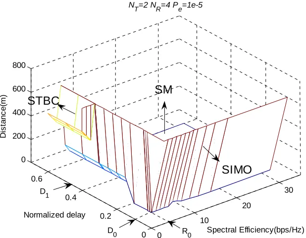
Figure 2.4 Switching bound based on spectral efficiency, delay and distance ... 30

Figure 2.5 Probability of selecting SIMO, STBC and SM... 31

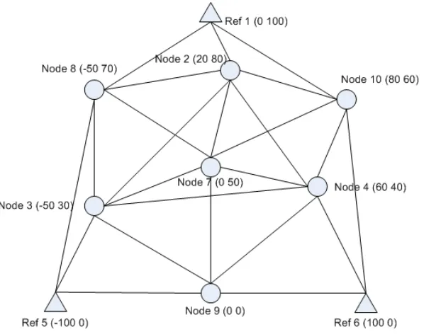
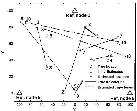
Figure 3.1 Topology of a simple network ... 44

Figure 3.2 Performance of joint localization and tracking ... 45

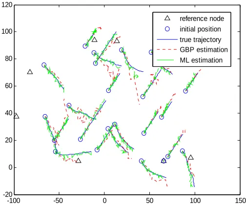
Figure 3.3 Snapshot of a random geometric network... 45

Figure 3.4 True and estimated trajectory of moving nodes... 46

Figure 3.5 Effect of node density on performance ... 48

Figure 3.6 Trade-off between communication and computation ... 49

Figure 3.7 Mean square error ratio with different particle numbers ... 50

Figure 4.1 Markov blanket (shaded nodes) and Markov blanket clusters (shaded clusters) for cluster C1. (reproduced Figure 1 in [40]) ... 63

Figure 4.2 Vertex Process (a), Edge Process (b) and Mixed Process (c) ... 68

Figure 4.3 State labeling of edge orocess on a 2-d torus... 70

Figure 4.4 Mean square error of estimation versus iteration number... 79

Figure 4.5 Mean square error of estimation versus communication energy ... 80

Figure 5.1 A factor graph example... 85

Figure 5.2 Factor graph structure for distributed clustering... 87

Figure 5.3 Factor graph structure of “mega-nodes” clustering ... 91

Figure 5.4 Ratio cut comparison with different network sizes... 94

Figure 5.5 Ratio cut comparison with different cluster sizes ... 95

Figure 5.6 Performance of distributed clustering for structured inferences-Convergence Rate ... 96

LIST OF ABBREVIATIONS AND ACRONYMS

AP affinity propagation AWGN additive white Gaussian noise BER bit error rate

BP belief propagation CP consensus propagation

GBP Gaussian particle filtering Belief Propagation algorithm GPF Gaussian particle filtering

i.i.d. independent and identically distributed KL Kullback–Leibler

MA mobile agent

MAP maximum a posterior MIMO multi-input multi-output ML maximum likelihood MSE mean square error

MMSE minimum mean square error MRF Markov random fields MRC maximum ratio combining PEP pairwise error probability pdf probability density function QAM quadrature amplitude modulation RSS received signal strength

SENMA sensor networks with mobile agents SIMO single-input multi-output

SISO single-input single-output SM spatial multiplexing

Chapter 1

Introduction

1.1. Collaborative Information Processing in Distributed

Wireless Networks

Recent advances in information technology are leading to a paradigm shift towards ad hoc networking, distributed processing and pervasive computing and communications. Examples include mobile ad hoc networks, wireless mesh networks, and sensor networks for various military, commercial, environmental and emergency applications. Due to rapid development in signal processing, networking and MEMS technologies, these networks are playing an increasingly important role in our life [1]. Such kinds of large-scale wireless networked systems consisting of small devices (nodes) capable of sensing, computing, and wireless communication are referred to as distributed wireless networks in this dissertation, or wireless networks for short, in contrast to the traditional infrastructure-based wireless networks, such as cellular networks and wireless LANs (WLAN).

exhibit daunting global behavior, a phenomenon already observed in many biological systems. For anticipated applications, cooperative schemes that are distributed, robust, scalable, and energy-efficient, are much desired.

In general, distributed and cooperative information processing can be conducted with two infrastructures: a hierarchical one where data are collected and transmitted to some fusion centers for central processing, without excluding the possibility of local processing and coordination among nodes; and a flat one where the global computing is effectively distributed in the whole network solely via local information exchange. This dissertation investigates both of these infrastructures, but mostly focuses on the latter one, which is far less explored, and expected to be both more challenging and more fruitful.

While collaborative communication and information processing in distributed wireless networks is a very active research area, many problems remain open and a general design framework is lacking. This constitutes the motivation for this dissertation, where we address some important issues of this broad topic, including cooperative transmission, distributed localization and tracking, distributed inference and distributed clustering. In subsequent sections of this chapter, we give a more detailed introduction of each sub-topic treated this dissertation.

1.2. Energy Efficiency and Transmission Strategy Selection

[3] and references therein). Specifically, by allowing sensor nodes in close proximity to cooperate in transmission to form a virtual multiple-input multiple-output (MIMO) system, recent progress in wireless MIMO communications can be exploited to boost the system throughput, or equivalently reduce the energy consumption for the same throughput and BER target. However, these cooperative transmission strategies may incur additional energy cost and system overhead. In the first part of this dissertation, by assuming that data collectors are equipped with antenna arrays and superior processing capability, we study energy efficiency of relevant traditional and cooperative transmission strategies: Single-Input-Multi-Output (SIMO), Space-Time Block Coding (STBC) and Spatial Multiplexing (SM).

1.3. Distributed localization and Tracking in Wireless

Networks

Belief propagation (BP, also known as sum-product algorithm) refers to a general class of message-passing algorithms intended to solve the NP-hard probabilistic inference problems by exploiting “partial independence” existing among random variables [4]. Having succeeded in many diverse fields, BP has also been considered for wireless networks very recently [5]. Arguably, wireless ad hoc and sensor networks provide an excellent arena for BP algorithms, where a large number of nodes are only weakly and locally coupled, and where dominating applications are to draw inference or compute functions based on the whole collection of data. On the other hand, BP supplies a general and flexible framework for collaborative information and signal processing in wireless networks.

However, infeasible computation and communication requirements involved in applications entailing non-discrete distributions limits its use in practical situations with resource constraints. Particle filtering techniques (or sequential Monte Carlo) [6] can be exploited to tackle these issues, involving particle-based approximation and importance sampling. The basic idea is to represent relevant continuous distributions with a list of mass points (“particles”) together with the associated weights. This approach turns the integral form of messages into weighted sums of functions, and importance sampling techniques can be applied to further transform the messages into particles or more general sample-based density estimates, thus suitable for transmission.

achieve predetermined goals. In the second part of this dissertation, we apply this idea of particle-based belief propagation for the distributed localization and tracking problems. Particularly, we proposed a distributed self-localization algorithm based on particle-based belief propagation, for which the majority of nodes determine their own locations through range estimates between themselves and their neighbors, and through the aid of a few reference nodes (i.e., nodes with known coordinates).

1.4. Distributed Inference in Wireless Networks

Distributed inference is the primary task of a wide range of wireless networking applications, like localization, tracking and time synchronization. In general, the objective of distributed inference is to compute marginal posterior probabilities through local interactions among nodes, given a set of observations and some underlying graph model. Message passing algorithms, like belief propagation are attractive for distributed inference in wireless sensor networks (WSN) due to their energy efficiency, robustness and scalability [2].

In the third part, we proposed a variational message passing framework for Markov random fields, which is computationally more efficient and admits wider applicability compared to the traditional approaches. Distributed inference on a flat infrastructure enjoys the benefits of simplicity and uniformity in message formation, while higher accuracy and faster convergence can usually be achieved by organizing the whole network into a more structured one. In this part, we further investigate exploiting substructures of networks to improve variational methods in real systems. Thus the simplicity of variational methods (for inter-cluster processing) and the high accuracy of exact inference algorithms (for intra-cluster processing) can be exploited simultaneously. To our knowledge, this is the first work to explicitly apply the structured variational methods for distributed inference in wireless networks.

overall performance is quantitatively characterized via the coupling approach. A tradeoff between complexity and performance of this algorithm is analytically addressed, which provides important insights and guidelines for the system analysis and design.

1.5. Distributed Network Decomposition

Aiming to minimize the sum of cut weights between different clusters of nodes, network decomposition, or graph partition, lies in the core of a wide range of data processing and networking applications, like pattern recognition, load balancing and parallel computation. Especially, it offers flexibility for distributed inference in wireless networks, which we discussed previously. However, this problem is NP-hard in general, while the current approximate solutions - spectral clustering algorithm and semi-definite programming relaxation suffer from complicated computations and the requirement of global knowledge.

1.6. Dissertation Outline

Chapter 2

Energy-Efficiency and Optimal Transmission

Strategy Selection

2.1. Introduction

Energy efficiency is one of the most critical concerns for sensor applications [9]. Direct communications between sensor nodes and the (possibly) distant data collector is in general energy inefficient, as each node needs to transmit highly redundant data. By allowing sensor nodes in close proximity to cooperate on communication, not only can the collected data be efficiently fused, but recent progress in wireless multi-input multi-output (MIMO) communications can be exploited to boost the system throughput, or equivalently reduce the energy consumption for the same throughput and bit error rate (BER) target.

which consumes extra energy and induces additional delay. Therefore, it may not always be better to enforce cooperative transmission and vice versa. Determination of the optimal transmission strategy depends on many interacting factors including system demand, network topology, and availability of channel information.

Energy analysis on cooperative MIMO in sensor networks was investigated in [10], where it is shown that the Alamouti space-time block coding (STBC) scheme on a cooperative 2 2× MIMO is more energy efficient than the traditional single-input single-output (SISO) approach when the transmission distance is larger than a small threshold. [11] and [12] extend the idea of virtual MIMO to the V-BLAST (or more general spatial multiplexing (SM)) architecture. In [13], the authors consider the energy efficiency of cooperative STBC with the low-energy adaptive clustering hierarchy (LEACH) protocol. An explicit distance threshold over which cooperative transmission is advantageous is given. Synchronization problem is also addressed. More recent work in this subject [14] endeavors to investigate the diversity-multiplexing trade-off [15] considering the energy consumption. Their results show that both diversity and multiplexing gain should be exploited to obtain optimal energy efficiency.

(potentially more capable) collecting node or base station within a given period. Secondly, we provide a unified and practical framework to analyze and compare the energy efficiency of various transmission strategies in wireless sensor networks. And lastly, we take an initial step to quantify the switching thresholds among three representative transmission strategies: traditional non-cooperative transmission, space-time block coding, and spatial multiplexing, the latter two of which fall within the cooperative transmission category yet are feasible to implement for sensor applications. The selection rules are decided such that the best energy efficiency is achieved with given system or link level demand or knowledge.

The rest of this chapter is organized as follows. Section 2.2 presents the system model and our assumptions for analysis. Energy efficiency of relevant transmission strategies is studied in Section 2.3, which provides a basis for selection of energy-efficient signaling. Then in Section 2.4 and 2.5, general guidelines are proposed for optimal transmission strategy selection in some typical scenarios, based on system-level demand and link-level knowledge, respectively. Some numerical results are given in Section 2.6. Finally Section 2.7 contains some concluding remarks.

2.2. System Model

2.2.1.

Channel Model

through high-speed connections. Examples of mobile agents include manned/unmanned airplanes or vehicles, or specially designed light nodes that can hop around in the network. In this section, we further investigate the possible advantages of cooperative MIMO transmission in wireless sensor networks with mobile agents (SENMA), which can be similarly coined as M-SENMA.

We assume that at some moment N_T neighboring nodes in a SENMA intend to transmit to a designed MA equipped withN_R antennas. Independent frequency nonselective Rayleigh fading is assumed for the channels between each node and the MA, on top of the common path loss1. The equivalent discrete-time MIMO system can be described as

Y HX N= + , (2.1)

where Y is the received signal at the MA; X contains the substreams transmitted by the nodes; H is an NR×NT channel matrix, whose entries are modeled as independent and identically

distributed (i.i.d.) normalized complex Gaussian random variables; and N is the background noise, assumed to be circularly symmetric Gaussian with zero mean and variance N₀ for each component. The common path loss is incorporated in the power of X. It is assumed that slotted time division duplexing is employed for communication purposes. The optimal transmission strategy is decided at the MA, based on (available) relevant information at the system or link level, and fed back to the sensor group via a reverse signaling channel, which is also used to transmit beacons for synchronization purpose (as assumed in [16]).

As mentioned before, three basic transmission strategies are considered in this work: single-input multi-output (SIMO), which corresponds to traditional non-cooperative

1

transmission with the SENMA structure, STBC and SM, which exploit diversity and spatial multiplexing gains in MIMO systems, respectively [17]. In the cooperative STBC scheme,

T

N nodes collaborate to send out an N_T×p space-time block X with orthogonal rows to realize full diversity gain, where p represents the number of time slots in transmission. As is known, the maximum likelihood (ML) detection of each transmitted symbol is decoupled, equivalently represented as

y= H _F x+n, (2.2) where H _F, the Frobenius norm of H, is Gamma distributed with parameter N NT R and 1, and

the equivalent noise n still has varianceN0. It can be shown that the spectral efficiency (bits/s/Hz) of the STBC system is given by [17]

CSTBC(SNR)=rE⎡_⎢log 1

(

)

⎣ H ⎦, (2.3) where r is the code rate of STBC, E[x] denotes the expectation of a random quantity x, and SNR denotes the identical energy per user per block symbol divided byN₀. This expression should be compared to that of a SIMO system (corresponding to direct communications between a sensor node and an MA) with maximum ratio combining [17]

CSIMO(SNR)=E_⎣⎡log(1 |+ A| SNR)2 ⎤_⎦, (2.4) where|A|2is Gamma distributed with parameterN_R and 1. For the cooperative SM scheme, each sensor node sends an independent symbol each time, which can be viewed as a space-only code without loss of generality:

= +

y Hx n, (2.5) where y, x and n denote column vectors. The spectral efficiency of SM is given by [17]

where SNR is defined on the per-user basis as before to make a fair comparison.

2.2.2.

Energy Model

The transmit energy consumption per bit of a communication link is given by [18]

2 2 0

(4 ) np

b

TX r g

t r

E d

E N M

N G G

ξ π

η λ

⎛ ⎞

= _⎜ ⋅ _⎟

⎝ ⎠ , (2.7)

where E_b N₀ is the energy efficiency of signaling schemes to be discussed in the following,

r

N is the single-sided power spectral density of the receiver noise, (4 )π 2dn/G Gt rλ2 reflects

the end-to-end loss in transmission (n_pis the path loss exponential), M_g is the link budget margin, and /ξ η is a coefficient accounting for the RF power amplifier effect with ξ the peak-to-average ratio of the modulation scheme and η the drain efficiency of the amplifier.

CT C T

b

P

E N

R

= . (2.8)

To quantify the extra cost for cooperative MIMO transmission, we assume a simple cooperation protocol for illustration purpose, for which K_T out of N_T nodes have data to transmit (while others serve as relays). It is also assumed that cooperative nodes only communicate with one single MA at any moment, or they can choose the one with the best signal quality, as in the coverage of multiple MAs. Each of the K_T data nodes broadcasts its information to all the other nodes in this group using different time slots. The energy consumption per bit required for such cooperation is given as

, ( 1)

CT CR

CP T TX SISO T

b b

P P

E K E N

R R

⎛ ⎞

= _⎜ + + − _⎟

⎝ ⎠ (2.9)

2.3. Energy Efficiency of Non-Cooperative and Cooperative

Transmission

In this section, we first analyze the energy efficiency of several relevant transmission strategies in the wideband regime to obtain some insights, then turn to more realistic system settings.

2.3.1.

Wideband Asymptote

The wideband asymptotic analysis is to approximate the Shannon capacity C as an affine function of energy per bit normalized to the noise spectral density (i.e.,E_b/N₀) in the zero SNR neighborhood (corresponding to high-to-optimal energy efficiency) as [19]

( )

0 0min 0

log Eb log Eb C log 2 ( )

C o C

N = N +S + ,

2

(2.10)

where(E_b/N_{0 min}) is the (normalized) minimum required energy for reliable communications, and S0 stands for the wideband slope of the spectral efficiency-energy efficiency curve (in terms of bits/s/Hz/3dB). These two key parameters can be obtained as [19]

0 min

ln 2 (0)

b

E

N =β C ,

2 0

2 (0)

(0)

C S

C

⎡ ⎤

⎣ ⎦

=

− , (2.11)

with C, C the first and second derivatives of the spectral efficiency (e.g., (2.3), (2.4) and (2.6)) at SNR = 0, and β the parameter relating E_b/N₀, SNR and C(SNR) as

0

SNR (SNR)

b

E

N =βC , (2.12)

2

which equals to 1 for SIMO, r for STBC, and NT for SM. We summarize these two key

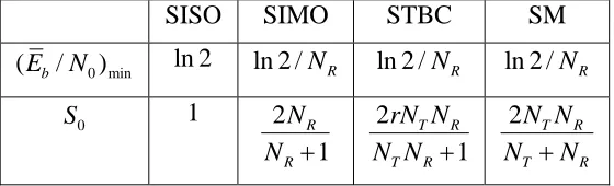
parameters for relevant transmission strategies (with Rayleigh fading) in Table 2-1.

Table 2-1 Wideband Analysis of Communications Systems Subject to Rayleigh Fading

SISO SIMO STBC SM

0 min

(E_b/N ) ln 2 ln 2 /N_R ln 2 /N_R ln 2 /N_R 0

S 1 2

1

R R

N N +

2

1

T R T R

rN N N N +

2 _{T R}

T R

N N N +N

Wideband analysis shows that receive diversity effectively lowers the minimum required energy by a factor of N_R. However, (E_b/N_{0 min}) alone does not reveal the whole picture as it could not differentiate various communication systems with receive antenna arrays but different transmit signaling. On the other hand, S₀ demonstrates their differences in spectral efficiency given certain energy efficiency in the wideband regime. In general, we have

1 2 2 2

1 1

R T R T R

R T R T R

N N N N N

N N N N N

≤ ≤ ≤

+ + + . (2.13)

0 1 2 3 4 5 6 7 -10

-9 -8 -7 -6 -5 -4 -3 -2 -1 0

Spectral Efficiency R/W (bits/s/Hz)

N

o

m

a

liz

e

d

E

n

erg

y

pe

r bi

t (dB

)

N_T=2 N_R=4

SISO

SIMO _STBC

SM

Figure 2.1 Wideband behaviors with Rayleigh fading

2.3.2.

Realistic Setting

decoding with polynomial complexity for SM systems [20]. The reader is referred to [12] for discussions of suboptimal detection methods for SM.

The average BER of an orthogonal STBC, following the performance analysis for diversity techniques in fading channels, can be very accurately approximated as [18] [21]

1 , 0 2 1

4 1 1 1

1

log 2 2

T R _{T R}

N N _{N N} l

T R e STBC

l

N N l

P l M M μ − μ = − + ⎛ ⎞ − + ⎛ ⎞⎛ ⎞ ⎛ ⎞ = _⎜ − _{⎟⎝⎜ ⎟ ⎜ ⎟⎜ ⎟} ⎠ ⎝ ⎠

⎝ ⎠

∑

with 1 α μ α =

+ and

2 0 3log 1 2( 1) b T E M

N M N

α =

− . (2.15)

For most applications of interest, we can further simplify (2.14) as

_,

2

2 1

4 1 1

1

log 4( 1)

T R N N T R e STBC T R N N P N N

M M α

− ⎛ ⎞ ⎛ ⎞ ⎛ ⎞ ≈ _⎜ − _{⎟⎜ ⎟ ⎜ ⎟} +

⎝ ⎠⎝ ⎠ ⎝ ⎠ . (2.16)

The required E_b/N₀ with target BER P_e for STBC can in turn be obtained as

1/

0 2 2

2 1

1 4 1

2( 1) 1

| 1

3log 4 log

T R N N T R T R b STBC T e N N N N

E M M

N

N M P M

⎛ _{⎛ ⎛ ⎞⎛ − ⎞⎞} ⎞ ⎜ _{⎜ ⎜} − _{⎟⎜ ⎟⎟} ⎟ − ⎜ ⎜ ⎝ ⎠⎝ ⎠⎟ ⎟ ≈ _{⎜ ⎜ ⎟} − _⎟ ⎜ _{⎜⎜ ⎟⎟} ⎟ ⎜ _{⎝ ⎠} ⎟ ⎝ ⎠

. (2.17)

Note that by taking N_T =1 in (2.17), we readily get the analytical results for a SIMO system with MRC, and further letting N_R =1 gives us results for SISO.

2 1 ₁ 0 2 1 1 ( ) ( ) 1 R R N _N R l j i l N P r l r − − = − ⎛ ⎞ ⎛ ⎞ → =_{⎜ ⎟ ⎜ ⎟} + ⎝ ⎠

∑

x x , (2.18)

with

2

( / 2) / 2 1

r= Γ + Γ + Γ + and Γ = x_i−x_j 2/N₀. (2.19) Seeming different, (2.18) is actually the same as the average PEP for SIMO, given by (c.f. (2.14) withN_T =1)

1 0 1 1 1 ( ) 2 2 R _R

N _N l

R j i

l

N l

P x x

l μ − μ = − + ⎛ ⎞ − + ⎛ ⎞ ⎛ ⎞ → =_{⎜ ⎟ ⎜ ⎟⎜ ⎟}

⎝ ⎠

∑

when 1 1 r r μ = −

+ . (2.21) A detailed proof is given in Appendix A. After some algebra, (2.21) readily leads to

1 4

α = Γ(c.f. (2.15) and (2.19)), which in turn admits 2 ₂

2 min

6 log 1

i j b

M

d E

M

− = =

−

x x , (2.22)

the right hand side of which is readily recognized as the squared minimum distance of a square QAM symbol with average energy per bit E_b. Since error performance is typically dominated by the minimum-distance error events, we make the following assumption for the performance of equal-power and equal-rate SM with ML detection:

0 0

| |

b b

SM ML SIMO

E E

N − ≈ N , (2.23)

Based on the above analysis, we obtain the following simple linear relationship between energy efficiency and spectral efficiency for the three transmission strategies of interest, which bears a similar form as the wideband analysis (see Appendix B for details).

_{0 min}

0

log b | (1) (1)

SIMO

E

S R E

N ≈ + , (2.24)

0

min 0

(1)

log b | ( )

STBC T

E S

R E N

N ≈ r + , (2.25)

0 min

0

log b | ( ) (1)

SM T

E

S N R E

N ≈ + , (2.26)

where

0

log 2 ( T)

T

S N

N

= , (2.27)

min

2 1

1

( _T) log( _T) log 4 T R _e

T R T R

N N

E N N P

N N N N

⎛ ⎛ − ⎞ ⎞

= + _{⎜ ⎜ ⎟ ⎟}

⎝ ⎠

⎝ ⎠. (2.28)

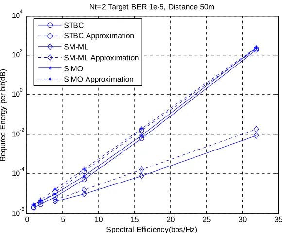
Note that again (2.24)~(2.26) are obtained with some simplifications. Nonetheless it is sufficient for our study and further verified through simulations. An example is given in Figure 2.2, where transmission energy E_TX of the three transmission strategies as a function of spectral efficiency is plotted (see Section VI for parameter settings). Qualitatively similar observations as revealed in the wideband analysis are made here: compared with SIMO, STBC lowers the required energy by exploiting the diversity gain, whose potential is somewhat limited; in contrast, multiplexing gain in SM improves the system energy efficiency by orders of magnitude3, when high spectral efficiency is also desired.

3

0 5 10 15 20 25 30 35 10-6

10-4 10-2 100 102 104

Spectral Efficiency(bps/Hz)

R

e

qu

ir

e

d E

n

er

gy

pe

r

bi

t(

d

B

)

Nt=2 Target BER 1e-5, Distance 50m

STBC

STBC Approximation SM-ML

SM-ML Approximation SIMO

SIMO Approximation

Figure 2.2 Transmit energy comparison with different spectral efficiency

2.4. Optimal Transmission Strategy Selection – System

Level

2.4.1.

Given Transmission Distance

Suppose the distance between the sensor nodes and the MA d is given, and our objective is to find the most energy efficient transmission strategy with no other constraints. In this scenario SM is beyond consideration when spectral efficiency or delay is not a concern; the other two schemes will employ BPSK to save energy consumption. Denote the corresponding spectral efficiency as R_min. If the transmit energy dominates (i.e., circuit energy consumption and cooperation penalty is relatively negligible), it turns out that STBC is always the best, as

min( T)

E N is a decreasing function of N_T.

Criterion 1a: Regarding transmit energy consumption, for any transmission distance, the optimal transmission strategy is STBC.

If circuit energy consumption and cooperation penalty can not be ignored, it is expected that for small transmission distance, the saving of STBC in transmit energy can not justify the extra costs. By solving E_{TX SIMO,} +E_{C SIMO,} +E_{CP SIMO,} <E_{TX STBC,} +E_{C STBC,} +E_{CP STBC,} with respect to distance, the selection criterion is obtained as follows.

Criterion 1b: Regarding total energy consumption, given a transmission distance d, choose SIMO when

(

)

min

min min

1

1 / _{(1) ( )} 1/

min

2 ₍ T ₎

th R n _{E E N} n

d d

e e R

β α

< =

− , (2.29)

where

1/ 2

2

(4 )

n t r

r g

G G

N M B

λ η α

ξ π

⎛ ⎞

= ⎜_⎜ ⎟_⎟

⎝ ⎠ , (2.30)

1

(

)

n T CT T CR

N P N P

and choose STBC otherwise.

2.4.2.

Spectral Efficiency Demand

In many applications a specific spectral efficiency demand R is also imposed, due to either the Quality-of-Service requirements or the network stability concerns. If only the transmit energy is concerned, STBC is uniformly better than SIMO for any spectral efficiency, and the switching threshold between STBC and SM turns out not to depend on the transmission distance (c.f. (2.25) and (2.26)).

Criterion 2a: Regarding transmit energy consumption, given a spectral efficiency demand R, choose STBC when

min min

0

0 0

(1) ( )

(1) ( )

T T

E E N

R R

S S N

− < =

− , (2.32)

and choose SM otherwise.

If the total energy consumption is considered, selection among the three schemes is more complicated and generally depends on the transmission distance as well. A key observation is that the switching threshold between STBC and SM is still given by (2.32) and is independent of d. The following selection criterion follows after some algebra.

Criterion 2b: Regarding total energy consumption, given a transmission distance d and a spectral efficiency demand R, whenR<R0, if transmission distance d satisfies (c.f.(2.29) ~(2.31))

(

)

1

1 / _{(1) ( )} 1/

2 ₍ T ₎

th R n _{E E N} n

d d

e e R

β α

′ < =

− , (2.33)

(

)

min

2

2 (1) / _/ 1/

(2 2 T)

th E n _{R R N} n

d d

e _R

β α

< =

− , (2.34)

where

β₂ =

(

)

2.4.3.

Delay Constraint

In some scenarios (emergency or real-time applications) a hard limit is put on the total transmission delay. As one expects, the delay constraints are closely related to spectral efficiency demands. From the definition of cooperative MIMO transmission strategies, they can be explicitly derived as below:

SIMO s SIMO

N

T T

R

= , (2.36)

,

STBC s

STBC STBC l

N N

T T

R R

⎛ ⎞

= ⎜_⎜ + ⎟_⎟

⎝ ⎠, (2.37)

, ( _T 1) / _T

SM s

SM SM l

N N N

N

T T

R R

⎛ ₋ ⎞

= _⎜⎜ + _⎟⎟

⎝ ⎠, (2.38)

where N is the total number of bits to be transmitted, T_s is the symbol duration, R denotes the spectral efficiency for long-haul transmission while R_,l stands for local cooperation4. The second terms in T_STBC and T_SM represent the additional delay incurred by cooperation. Therefore, for each given spectral efficiency-delay pair, there is an achievable region dictated by (2.36), (2.37) and (2.38), beyond which one has to meet one while violating the other. Another point worth noting is that, if the delay constraint is too stringent, then local

4

cooperation can not be afforded, and SIMO becomes the only choice. By defining the average normalized delay per bit D=T T N/( _s ) to remove the system dependence, we formalize the selection rule for a given D below. For simplicity we assume the spectral efficiency for local transmission is the same for STBC and SM, denoted asR_l. Substituting the above equations into(2.24), (2.25) and (2.26) leads to the relationship of delay and energy efficiency for different transmission strategies:

0

min 0

(1)

log b | (1)

SIMO

SIMO

E S

E

N = D + , (2.39)

0

min 0

(1)

log | ( )

1 b STBC T STBC l E S E N N _D R = + −

, (2.40)

0

min 0

( )

log | (1)

( 1) /

b T

SM

T T

SM

l

E S N

E N N N D R = + − −

. (2.41)

From (2.39), (2.40) and (2.41), a tradeoff between delay and energy consumption can be observed. Stringent delay requirement results in large energy consumption. With delay constraint relaxed, more energy savings can be achieved. Similarly, by solving the cross-points of delay-energy curves, we can get the following switching criterion.

Criterion 3: Regarding transmit energy consumption, given a delay constraintD, choose SIMO when 0 1 l D D R

< = , (2.42)

choose STBC when (cf. (2.32))

₁ 0 1 1 l D D R R

The selection criteria regarding total energy consumption and joint delay-distance consideration can be similarly addressed and the details are omitted here since they don’t provide further insights.

2.5. Optimal Transmission Strategy Selection – Link Level

In certain circumstances, when the channel is quasi-static and sufficient feedback is affordable, transmission strategies can be determined based on instantaneous channel characteristics. The problem of switching between STBC and SM to minimize the error rate has been addressed in [23] [24]. Here we extend the work to selecting among STBC, SM or SIMO to minimize the required transmit energy for a given BER and spectral efficiency. The problem regarding total energy consumption minimization follows a similar approach as discussed above and thus will not be explicitly addressed here.

With an MRC receiver, the (conditional) error rate for SIMO is bounded as [17]

2

| 2 min,

|

0

( ) || ||

2

s SIMO SIMO e SIMO SIMO e SIMO

E d

P N Q

N

⎛ ⎞

⎜ ⎟

≤

⎜ ⎟

⎝ ⎠

h h , (2.44)

where N_e is the average number of nearest neighbors in constellation, E_{s SIMO|} is energy per symbol per transmit antenna,||h_SIMO||2 is the squared norm of the channel, and d_min,SIMO is the minimum distance of a unit-energy symbol. For a target P_e and spectral efficiency R, we have

2 1

0

2 2

min, 2 |

|| ||

e b SIMO

SIMO SIMO e

N P

E Q

d R N

−

⎛ ⎛ ⎞⎞

≥ _{⎜⎜ ⎜ ⎟⎟⎟}

⎝ ⎠

⎝ ⎠

2

| 2 min,

|

1 0

( ) max || ||

2

T

s STBC STBC e

e STBC MIMO k

k N

E d

P N Q h

N ≤ ≤

⎛ ⎞

⎜ ⎟

≤

⎜ ⎟

⎝ ⎠

H , (2.46)

where h_k is the kth column of H_MIMO, and other symbols are defined as before. It is known

that 2 _max2

1max ||t || ( )

k MIMO

k N h λ

≤ ≤ ≤ H , whereλmax(HMIMO) is the maximum singular value of the

channel. So we have

2 1 0 2 2 min, max 2 | ( ) T e b STBC

STBC MIMO e

N N P

E Q

d λ R N

−

⎛ ⎛ ⎞⎞

≥ _{⎜⎜ ⎜ ⎟⎟⎟}

⎝ ⎠

⎝ ⎠

H . (2.47)

An upper bound of the (conditional) BER for SM with ML detection is given by [23]

2 2 min min, 0 ( ) | | ( ) 2 MIMO SM s SM

e SM MIMO e

T

d E

P N Q

N N λ ⎛ ⎞ ⎜ ⎟ ≤ ⎜ ⎟ ⎝ ⎠ H

H , (2.48)

where λ_min(H_MIMO) is the minimum singular value of the channel, from which we can obtain 2 2 1 0 2 2 min, min 2 | ( ) T e b SM

SM MIMO e

N N P

E Q

d λ R N

−

⎛ ⎛ ⎞⎞

≥ _{⎜⎜ ⎜ ⎟⎟⎟}

⎝ ⎠

⎝ ⎠

H . (2.49) Based on these results, a qualitative selection rule is given below.

Criterion 4: Regarding transmit energy consumption, when instantaneous channel information is available, choose the scheme that makes the corresponding metricd_min,SIMO||h_SIMO||, min,STBC max( MIMO)

T

d

N

λ H

, min,SM min( MIMO)

T

d

N

λ H

largest5.

2.6. Numerical Results

In this section, some numerical examples are provided to better illustrate our main results above. In simulations, a real system operating at 2.5GHz is assumed with bandwidth B=10

kHz. The following values are taken for the parameters in Equation (2.7); η =0.35,

161 /

r

N = − dBm Hz, 5G G_{t r} = dBi and M_g =40dB. For square QAM we have

max 3( 1)

( 1)

av

M

M

ξ = = −

+

E

E . (2.50)

The typical energy consumption values of various circuit blocks are quoted from [10], with 97.8

CT

P = mw and P_CR =112.8mw.

First, the switching bounds given spectral efficiency demand and transmission distance are illustrated for some values of NT in Figure 2.3. Based on Criterion 2a, the potential

transmission scheme category (STBC/SIMO or SM/SIMO) is determined by R₀(c.f. (2.32)), while the distance thresholds are plotted according to Criterion 2b (c.f. (2.33) and (2.34)). Delimited by these thresholds, the preferable working regions of different transmission strategies are indicated in the figure (by arrows). It can be seen that with spectral efficiency growing, the curves converge to the x-axis. So the system tends to have only one choice: SM. Also note that since the advantage of STBC over SIMO in terms of transmit energy is somewhat limited, it overtakes SIMO only for a large distance.

0 2 4 6 8 10 12 14 0

100 200 300 400 500 600 700 800 900 1000

Spectral Efficiency(bps/Hz)

D

ist

a

n

ce

(m

)

N_R=4 P_e=1e-5

N_T=8 N_T=4 N_T=2

R₀ threshold

STBC

SM

SIMO

Figure 2.3 Switching bound based on spectral efficiency and distance

0

10

20

30

0 0.2

0.4 0.6

0 200 400 600 800

Spectral Efficiency(bps/Hz)

N

T=2 NR=4 Pe=1e-5

Normalized delay

D

is

tanc

e(m

)

SIMO SM

STBC

R

0

D

0

D

1

Finally, we illustrate the link-level selection criterion by studying the statistical probabilities of selecting SM, STBC and SIMO with different spectral efficiency demands. In Figure 2.5, it is seen that the probability of choosing SM tends to be 1 as spectral efficiency demand grows.

0 2 4 6 8 10 12 14 16 18 20

0 0.1 0.2 0.3 0.4 0.5 0.6 0.7 0.8 0.9 1

Spectral Efficiency(bps/Hz)

P

robab

ilit

y

N

T=2 NR=2

Prob. of selecting SIMO Prob. of selecting STBC Prob. of selecting SM

Figure 2.5 Probability of selecting SIMO, STBC and SM

2.7. Summary

Chapter 3

Cooperative Self-Calibration via Particle Belief

Propagation

3.1. Introduction

In recent years, belief propagation (BP) [4], which has proved successful in artificial intelligence, computer vision, and coding, attracts more and more attention in wireless network research. Distributed in nature, BP also possesses many other advantages in scalability, robustness, and energy-efficiency, demonstrating tremendous potential to facilitate probabilistic inference and signal processing in collaborative wireless networks [2].

Despite these desirable features, it’s not straightforward to employ BP algorithms for distributed communication and processing in wireless networks involving continuous distributions (e.g., estimation, localization and tracking): the message construction often involves intractable integrals, and we can not send out messages of infinite dimensions. One can simply recourse to discretization, which may not be efficient, especially for problems with large range or high dimension.

(e.g., [25] [26] [28]), but much is left to be done. In particular, depending on applications, the involved computations may still be prohibitive, should thousands of particles be required. This further increases the communication cost when distribution-related messages need to be exchanged in the network (e.g., as dictated by the BP algorithm).

Incorporating particle filtering into BP was pioneered by [8], and applied to the (static) self-localization problem in sensor networks in [5]. The location information of mobile portable devices is necessary for various emerging applications like E911 emergence service and ubiquitous computing. It is also indispensable for wireless sensor networks, in order for sensor nodes to self-organize and collaborate to achieve predetermined goals. A distributed self-localization algorithm such as that in [5] is of great interest, for which the majority of nodes determine their own locations through range estimates between themselves and their neighbors, and through the aid of a few reference nodes (i.e., nodes with known coordinates).

further reduce communication and computation requirement, and achieves favorable performance with moderate system turbulence. We also explore the idea of neighboring node selection to further reduce communication cost.

The rest part of this chapter is organized as follows: Section 3.2 describes the system models and formulates the problem. The proposed dynamic self-calibration algorithm based on BP with Gaussian particle filtering is presented in Section 3.3. In Section 3.4, some simulation results are given. Section 3.5 concludes the chapter.

3.2. System Models and Problem Statement

3.2.1.

Motion Model

Suppose we have S nodes in the field. The state variable of interest contains each node’s position p and velocity v, denoted as x_i =[p v_i, ]_i T, 1≤ ≤i S. A commonly used discrete-time model (e.g. [28]) is assumed for the time evolvement of the state variables:

X_n+1 =ΦX_n+ΩW_n, (3.1)

where the state vector 1, ,..., ,

T n = ⎣⎡ n S n⎤⎦

X x x , with _, [ _, , _, ] ,T i n = pi n vi n

x collects the positions and velocities of S nodes (both are complex comprising 2-D coordinates) at time n;

Φ

⎡ ⎤

⎢ _Φ ⎥

⎢ ⎥

=

⎢ ⎥

⎢ _Φ⎥

⎣ ⎦

0 0

0 0

Φ

0 0

,

Ω

⎡ ⎤

⎢ _Ω ⎥

⎢ ⎥

=

⎢ ⎥

⎢ _Ω⎥

⎣ ⎦

0 0

0 0

Ω

0 0

with 1

0 1

s

T

⎡ ⎤

Φ = ⎢ ⎥

⎣ ⎦ ,

2

/ 2

s s

T

T

⎡ ⎤

Ω = ⎢ ⎥

⎣ ⎦ (where Ts is the sampling period);

1, 2, ,

T n = ⎣⎡W n W n WS n⎤⎦

W stands for acceleration turbulence and its components are typically modeled as Gaussian with zero mean and covariance matrix

2 2 2

11 12 1

2 2 2

21 22 2

2 2 2

1 2

S S

S S SS

C

σ σ σ

σ σ σ

σ σ σ

⎡ ⎤

⎢ ⎥

⎢ ⎥

=

⎢ ⎥

⎢ ⎥

⎢ ⎥

⎣ ⎦

.

3.2.2.

Distance Measurement Model

For range measurement, received signal strength (RSS) is commonly used considering node complexity and cost. In this paper, we follow the same assumption as in [5], i.e. node i obtains a noisy measurement of its distance d_ij to its neighboring node j as

d_ij =|p_i−p_j|+v_o, (3.2)

where the observation noise vo ~N(0,σo2) is Gaussian. Extension to more general communication models and other ranging techniques is straightforward.

3.2.3.

Problem Formulation

1

( ,... ,...i S, | ij, ( , ) )

p x x x i V d∈ i j ∈E . (3.3)

By Markovian assumptions on { }x_i (thus the network can be regarded as a Markov random field), we can turn to find the marginals

( i| j, ij, i) ( i| ij, ( , ) )

p x x d j∈Γ ∝ p x d i j ∈E , i V∈ , (3.4)

where Γi stands for the set of neighbor nodes of i, without calculating the joint probability

(3.3). This kind of problems essentially falls into the targeted category of belief propagation algorithm.

3.3. Gaussian Particle Filtering based Belief Propagation

for Self-Calibration

3.3.1.

Belief Propagation Algorithm

Belief propagation is a class of distributed algorithms, originally intended to solve the NP-hard probabilistic inference problems by exploiting “partial dependence” among the random variables. The essence of the BP algorithm is the message-passing rule and belief-updating rule. Given the potential function φ_i( )x_i for each node i and the compatibility functionψ_ij( ,x x_{i j})for each pair of neighboring nodes( , )i j , the message from node i to j at the kth iteration is a function ofx_j, defined as

1 1

1 \

( )

( ) ( , ) ( ) ( ) ( , ) ,

( )

i

k

k k i i

ij j ij i j i i ki i i ij i j k i

k j ji i

b

m m d d

m

ψ φ − ψ −

− ∈Γ

∝

∫

∏

∫

x x x x x x x x x

x (3.5)

the current belief (approximated posterior probability distribution) that node i has about xj,

given its own observations and received messages from other parts of the graph in the last round. The belief node i has about its own variable is updated as

( ) ( ) ( ) i

k k

i i i i ji i j

b φ m

∈Γ

∝

∏

x x x . (3.6)

For our problem, the node potential function assumes the prior distribution of the state variable x_i (uniform if no priors are available), i.e.,

( )φ_i x_i = p( )x_i , (3.7) while the compatibility function is set based on the mutual distance measurement, i.e.,

(

)

( , )

o

ij i j pv dij i j

ψ x x = − p −p , (3.8)

where in this paper ~ (0, 2) o

v o

p N σ denotes the conditional probability of the observed distance given node location information.

3.3.2.

Belief Propagation with Gaussian Particle Filtering

The key idea of Gaussian particle filtering is to perform the filtering through particles while approximating the posterior distribution by single Gaussians. Hence, in the computation at each node, particle-based approximations and importance sampling are exploited to simplify calculations. The obtained particles for outgoing messages, however, are transformed into Gaussian distributions, and only the means and the variances are propagated among nodes.

Denote byN( ; , )x μ Σ a Gaussian distribution for random variable vectorx with mean vector μ and covariance matrix Σ. Suppose at the end of the kth iteration for time n, the message from node i to its neighbor node j is N( ;x μ_{ij n}k_, ,Σk_{ij n,} ), and the belief of node i is

, ,

( ;x μk_{i n},Σk_{i n})

N . Without loss of generality, it is assumed that κ iterations of the BP algorithm are executed for each time interval. At the beginning of a time instant, we draw samples {x_{i n}0( )_,m}_mM₌₁ and {x1( )_{ij n,}m}_mM₌₁uniformly from N( ;x μκ_{i n, −1},Σκ_{i n, −1}) and N( ;x μκ_{ij n, −1},Σκ_{ij n, −1}), respectively; and if either node is moving, new estimates are obtained through state evolvement equation (3.1). In the following iterations, samples {xk m_{i n,}( )}M_m=1 and {x_{ij n}(k_,+1)( )m}M_m=1

are drawn uniformly from N( ;x μki n_, ,Σki n_, ) and ( ; , , , )

k k ij n ij n

x μ Σ

N , respectively.

In general, at the start of iteration (k+1) for time n , given M samples (particles)

( ) , 1

{xk m_{i n} }M_m= and {x(_{ij n}k_,+1)( )m}M_m=1, the message composition step in the BP algorithm becomes6

6 ()

, ( , )

k k m ji n i n

m x stands for the value of ( ; , , , )

k k ji n ji n

xμ Σ

N at point ( )

,

k m i n

, 1 , , ( ) , 1 . ( ) , ( ) 1 , ,

( ) ( ) ( , ) ( ) ( ) ( , ) ( ) ( , ) . ( ) k i n i k

ij n j ij i j k i ji n i M

k m i i n m

ij i j k i

ji n i k m

M

ij i n j k k m m ji n i n

b m d m d m m ψ δ ψ ψ + = = ∝ − = =

∫

∑

∫

∑

x x x x

x x x

x x x

x x x

x

(3.9)

Considering the compatibility function given in (3.8), the associated weights for new message particles ( 1)( )

, 1

{ k m}M

ij n m

+ =

x can be easily obtained as

(

)

( 1)( ) ( ) ( 1)( ) ( )

, _o , , , / , ( , )

k m k m k m k k m

ij n v ij n i n ij n ji n i n

w + = p d − p − p + m x . (3.10)

For the purpose of numerical stability, a normalization step is necessary:

(_, 1)( ) (_, 1)( ) (_, 1)( ) 1

/

M

k m k m k m

ij n ij n ij n m

w + w + w +

=

=

∑

In the spirit of Gaussian particle filtering, the mean and variance of the outgoing message are computed recursively as

1 ( 1)( ) ( 1)( )

, , ,

1

M

k k m k m

ij n ij n ij n m

w

+ + +

= =

∑

μ x , (3.12)

_,1 (_, 1)( ) _,1 (_, 1)( ) _,1 (_, 1)( ) 1

( )( )

M

k k m k k m k k m H

ij n ij n ij n ij n ij n ij n m

w

+ + + + + +

=

=

∑

Σ μ x μ x . (3.13)

Besides ease of transmission, this Gaussian distribution is also used for particle sampling in the next iteration.