Proficient Cache-Supported Path Preparation on Roads

(1)

Available online: https://edupediapublications.org/journals/index.php/IJR/ P a g e |

4447

Proficient Cache-Supported Path Preparation on Roads

Boya Ganesh

,

S.G. Nawaz

2

, R. Ramachandra

3

1

_{Dept of CSE,}

_{Sri Krishnadevaraya Engineering College, Gooty, Andhra Pradesh}

2

_{Associate Professor,Dept of CSE,}

_{Sri Krishnadevaraya Engineering College, Gooty, Andhra Pradesh}

3

_Professor&

_Principa

_{l,Dept of Mech,}

_{Sri Krishnadevaraya Engineering College, Gooty, Andhra Pradesh}

Email:

saiganeshkumar2@ Gmail.com

1

Abstract: Path planning problems greatly arise in many applications where the objective is to find the shortest path from a given source to destination. In this paper, we explore the comparison of programming languages in the context of parallel workload analysis. We characterize parallel versions of path planning algorithms, such as the Dijkstra’s Algorithm, across C/C++ and Python languages. Programming language comparisons are done to analyze fine grain scalability and efficiency using a single socket shared memory multicore processor. Architectural studies, such as understanding cache effects, are also undertaken to analyze bottlenecks for each parallelization strategy. Our results show that a right parallelization strategy for path planning yields scalability on a commercial multicore processor. However, several shortcomings exist in the parallel Python language that must be accounted for by HPC researchers.

Index Terms:Spatial database, path planning, cache

I. INTRODUCTION

Due to advances in big data analytics, there is a growing need for scalable parallel algorithms. These algorithms encompass many domains including graph processing, machine learning, and signal processing. However, one of the most challenging algorithms lie in graph processing. Graph algorithms are known to exhibit low locality, data dependence memory accesses, and high memory requirements. Even their parallel versions do not scale seamlessly, with bottlenecks stemming from architectural constraints, such as cache effects and on-chip network traffic.

Path Planning algorithms, such as the famous Dijkstra’s algorithm, fall in the domain of graph analytics, and exhibit similar issues. These algorithms are given a graph containing many vertices, with some neighboring vertices to ensure connectivity, and are tasked with finding the shortest path from a given source vertex to a destination vertex. Parallel implementations assign a set of vertices or neighboring vertices to threads, depending on the parallelization strategy. These strategies naturally introduce input dependence. Uncertainty in selecting the subsequent vertex to jump to, results in low locality for data accesses.

Moreover, threads converging onto the same neighboring vertex sequentialize procedures due to synchronization and communication. Partitioned data structures and shared variables ping-pong within on-chip caches, causing coherence bottlenecks. All these mentioned issues make parallel path planning a challenge.

Prior works have explored parallel path planning problems from various architectural angles. Path planning algorithms have been implemented in graph frameworks. These distributed settings mostly involve large clusters, and in some cases smaller clusters of CPUs. However, these works mostly optimize workloads across multiple sockets and nodes, and mostly constitute either complete shared memory or message passing (MPI) implementations. In the case of single node (or single-chip) setup, a great deal of work has been done for GPUs are a few examples to name a few.

These works analyze sources of bottlenecks and discuss ways to mitigate them. Summing up these works, we devise that most challenges remain in the fine-grain inner loops of path planning algorithms. We believe that analyzing and scaling path planning on single-chip setup can minimize the fine-grain bottlenecks. Since shared memory is efficient at the hardware level, we proceed with parallelization of the path planning workload for single-chip multi-cores. The single-chip parallel implementations can be scaled up at multiple nodes or clusters granularity, which we discuss. Furthermore, programming language variations for large scale processing also cause scalability issues that need to be analyzed effectively so far the most efficient parallel shared memory implementations for graph processing are in C/C++. However, due to security exploits and other potential vulnerabilities, other safe languages are commonly used in mission-deployed applications. Safe languages guarantee dynamic security checks that mitigate vulnerabilities, and provide ease of programming.

(2)

4448

overheads in the context of our parallel path planning workloads. This paper makes the following contributions:

We study sources of bottlenecks arising in parallel path planning workloads, such as input dependence and scalability, in the context of a single node, single chip setup.

We analyze issues arising from safe languages, in our case Python, and discuss what safe languages need to ensure for seamless scalability.

We plan to open source all characterized programs with the publication of this paper.

II. PATH PLANNING ALGORITHMS AND PARALLELIZATIONS

Dijkstra that is an optimal algorithm, is the de facto baseline used in path planning applications. However, several heuristic based variations exist that trade-off parameters such as parallelism and accuracy. ∆-stepping is one example

Fig.1. Dijkstra’s Algorithm Parallelization’s. Vertices allocated to threads shown in different colors.

which classifies graph vertices and processes them in different stages of the algorithm. The A*/D* algorithms are another example that use aggressive heuristics to prune out computational work (graph vertices), and only visit vertices that occur in the shortest path. In order to maintain optimality and a suitable baseline, we focus on Dijkstra’s algorithm in this paper.

A. Dijkstra’s Algorithm and Structure

Dijkstra’s algorithm consists of two main loops, an outer loop that traverses each graph vertex once, and an inner loop that traverses the neighboring vertices of the vertex selected by the outer loop. The most efficient generic implementation of Dijkstra’s algorithm utilizes a heap structure, and has a complexity of O(E + V logV). However,

in parallel implementations, queues are used instead of heaps, to reduce overheads associated with re-balancing the heap after each parallel iteration. Algorithm 1 shows the generic pseudo-code skeleton for Dijkstra’s algorithm. For each vertex, each neighboring vertex is visited and compared with other neighboring vertices in the context of distance from the source vertex (the starting vertex). The neighboring vertex with the minimum distance cost is selected as the next best vertex for the next outer loop iteration. The distances from the source vertex to the neighboring vertices are then updated in the program data structures, after which the algorithm repeats for the next selected vertex. A larger graph size means more outer loop iterations, while a large graph density means more inner loop iterations. Consequently, these iterations translate into parallelism, with the graph’s size and density dictating how much parallelism is exploitable. We discuss the parallelizations in subsequent subsections and show examples in Fig 1.

B. Inner Loop Parallelization

The inner loop in Algorithm 1 parallelizes the neighboring vertex checking. Each thread is given a set of neighboring vertices of the current vertex, and it computes a local minimum and updates that neighboring vertex’s distance. A master thread is then called to take all the local minimums, and reduce to find a global minimum, which becomes the next best vertex to jump to in the next outer loop iteration. Barriers are required between local minimum and global minimum reduction steps as the global minimums can only be calculated when the master thread has access to all the local minimums. Parallelism is therefore dependent on the graph density, i.e. the number of neighboring vertices per vertex. Sparse graphs constitute low density, and therefore cannot scale with this type of parallelization. Dense graphs having high densities are expected to scale in this case.

C. Outer Loop Parallelization

(3)

4449

1) Convergence Outer Loop Parallelization: The convergence based outer loop statically partitions the graph vertices to threads. Threads work on their allocated chunks independently, update tentative distance arrays, and update the final distance array once each thread completes work on its allocated vertices. The algorithm then repeats, until the final distance arrays stabilize, where the stabilization sets the convergence condition. Significant redundant work is involved as each vertex is computed upon multiple times during the course of this algorithm’s execution.

2) Ranged based Outer Loop Parallelization: The range based outer loop parallelization opens pare to fronts on vertices in each iteration. Vertices in these fronts are equally divided amongst threads to compute on, however, atomic clocks are still required due to vertex sharing. As pare to fronts are intelligently opened using the graph connectivity, a vertex can be safely relaxed just once during the course of the algorithm. Redundant work is therefore mitigated, while maintaining significant parallelism. However, as initial and final pare to fronts contain less vertices, limited parallelism is available during the initial and final phases of the algorithm. Higher parallelism is available during the middle phases of the algorithm. This algorithm’s available parallelism hereto follows a normal distribution, with time on the x-axis.

III. METHODS

This section outlines multicore machine configuration and programming methods used for analysis. We also explain the graph structures used for the various path planning workloads.

A. Many-core Real Machine Setups

We use Intel’s Core i7-4790 has well processor to analyze our workloads. The machine has 4 cores with 2-way hyper threading; an 8MB shared L3 cache, and a 256KB per-core private L2 cache.

B. Metrics and Programming Language Variations

We use C/C++ to create efficient implementations of our parallel path planning algorithms. We use the p thread parallel library, and enforce gcc/g++ compiler -O3 optimizations to ensure maximum performance. The p thread library is preferred over Open MP to allow for the use of lower level synchronization primitives and optimizations. For Python implementations, we use both threading and multiprocessing libraries to parallelize programs, with Python3 as the language version. We use these two parallelization paradigms to show the limitations and shortcomings in parallel safe language paradigms.

For each simulation run, we measure the Completion Time, i.e., the time in parallel region of the benchmark. The time is measured just before threads/processes are spawned/forked, and also after they are joined, after which the time difference is measured as the Completion Time. To ensure an unbiased comparison to sequential runs, we measure the Completion Time for only the parallelized code regions. These parallel completion times are compared with the best sequential implementations to compute speedups, as given by Eq (1). Values greater than 1 show speedups, while values between 0 and 1 depict slowdowns in addition to performance, memory effects in a specific parallelization strategy also affect scalability. To evaluate cache effects, the cache accesses are therefore measured using hardware performance counters.

Speedup = Sequential Time/Parallel Time (1)

C. Graph Input Data Sets and Structures

Synthetic graphs and datasets are generated using a modified version of the GT Graph generator, which uses RMAT graphs from Graph500. We also use real world graphs from the Stanford Large Network Dataset Collection (SNAP), such as road networks. These are undirected graphs, with a degree irregularly varying from 1 to 4. Generated graphs have random edge weights and connectivity. All graphs are represented in the form of adjacency lists, with one data structure containing the edge weights, and another for edge connectivity, and all values represented by integers. Both sparse and dense graphs are used to analyze parallelizations across different input types, as shown in Table I. We also scale synthetic graphs from 16K vertices to 1M vertices, and the graph density from 16 up to 8K connections per vertex.

TABLE I

SYNTHETIC GRAPHS USED FOR EVALUATION

IV. EXPERIMENTS

4.1 Dataset

(4)

4450

queries. Four sets of query logs with different distributions are used in the experiments: QLnormal and QLuniform are query logs with normal and uniform distributions, respectively.

QLcentral is used to simulate a large-scale event (e.g., the Olympics or the World Cup) held in a city. QLdirection is to simulate possible driving behavior (e.g., changing direction) based on a random walk method described as follows. We firstly randomly generate a query to be the initial navigational route. Next, we randomly draw a probability to determine the chance for a driver to change direction. The point of direction change is treated as a new source. This process is repeated until the anticipated numbers of queries are generated. The parameters used in our experiments are shown in Table 2.

4.2 Cache-Supported System Performance

4.2.1 Cache versus Non-Cache

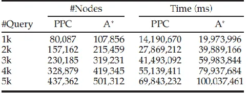
The main idea of a cache-supported system is to leverage the cached query results to answer a new query. Thus, we are interested in finding how much improvement our path planning system achieves over a conventional non-cache system. We generate query sets of various sizes to compare the paths generated by our PPC and A* algorithm. The performance is evaluated by two metrics: a) Total number of visited nodes: it counts the number of nodes visited by an

TABLE 2

Experimental Parameters

TABLE 3

Performance Comparison between PPC and the Non-Cache Algorithm

algorithm under comparison in computing a path, and b) Total query time: it is the total time an algorithm takes to compute the path. By default, we apply 3,000 randomly

generated queries to warm up the cache before proceeding to measure experimental results. Table 5 summarizes the statistics of the above two metrics with five different sized query sets. From the statistics we find that our cache-supported algorithm greatly reduces both the total visited nodes and the total query time. On average, PPC saves 23 percent of visiting nodes and 30.22 percent of response time compared with a non-cache system.

4.2.2 Cache with Different Mechanisms

Performance comparison: We further compare the performance of our system (PPC) with three other cache supported systems (LRU, LFU, SPC*) which adopt various cache replacement policies or cache lookup policies. The first two algorithms detect conventional (complete) cache hits when a new query is inserted, but update the cache contents using either the Latest Recent Used algorithm (denoted as LRU) or the Least-Frequently Used replacement policies (LFU), respectively. The third compared algorithm, namely, the shortest-path-cache (SPC*), is a state-of-the-art cache supported system specifically designed for path planning as PPC is. SPC* also detects if any historical queries in the cache match the new query perfectly, but it considers all sub-paths in historical query paths as historical queries as well. We compare these four cache mechanisms by converting the two metrics, number of visited nodes and response time, to saving ratios against non-cache system for better presentation

𝛿_node = nodes_{𝑐𝑎𝑐 ℎ𝑒}/nodes_{𝑛𝑜𝑛𝑐𝑎𝑐 ℎ𝑒}× 100% (2)

𝛿time = time𝑐𝑎𝑐 ℎ𝑒/time𝑛𝑜𝑛𝑐𝑎𝑐 ℎ𝑒× 100% (3)

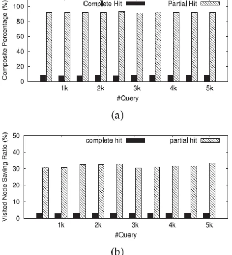
Visited node saving ratio and Query time saving ratio indicate how many nodes and how much time an algorithm can save from a non-cache routing algorithm (e.g., A*), respectively. A larger value indicates better performance. In the experiment, we increase the total query number from 1k to 5k and calculate the above two metrics using each cache mechanism with the results shown in Fig.2.

(5)

4451

Fig.2. Performance comparison with four cache mechanisms in terms of (a) visited node saving ratio, and (b) query time saving ratio with different numbers of queries.

As shown, our algorithm outperforms the other cache mechanisms in path planning significantly.

Performance analysis: In a cache-supported system, if the cached results can be (partially) reused, the server workload can be alleviated. Thus, we measure the hit ratio as follows:

𝛿_ℎ𝑖𝑡 = ℎ𝑖𝑡𝑠_{𝑐𝑎𝑐 ℎ𝑒}/|𝑄| × 100% (4)

where hitscache is the total number of hits and |Q| is the total number of queries. The hit ratio results using different cache mechanisms are compared in Fig. 3, from which we find that, as expected, PPC achieves a much higher hit ratio than the other three methods in all scenarios. We further analyze the correlation between the hit ratio and the performance metrics in terms of visited node saving ratio and query time saving ratio with the results shown in Fig. 4. From the figures, we make the following observations:

i. The visited node saving ratio and query time saving ratio are proportional to the hit ratio. Generally, with a higher hit ratio, the system performance improves as well. This is reasonable as the system does not need to re-compute the paths by analyzing the original road network graph, but retrieves the results directly from the cache when a cache hit occurs.

ii. However, saving ratios for visited nodes are not the same as for the query time. For example, PPC visits around 50 to 60 percent fewer nodes, but the response time saved is around 30 to 40 percent. A possible reason is that different nodes play different roles in the roadmap. When a query occurs at sub graphs with more complex structures, the routing usually takes longer as its computation may have more constraints than other nodes.

iii. The inconsistency above is particularly obvious in PPC, probably because PPC leverages partial hits to answer a new query. However, the remaining segments still need the computation from the road

Fig.3. Performance comparison with four cache replacement mechanisms in terms of hit ratio.

Fig.4. Correlation between (a) hit ratio and visited node saving ratio, and (b) hit ratio and query time saving ratio.

network graph, i.e., PPC does not always save sub paths if they require complex computations.

Because PPC leverages both complete and partial hit queries to answer a new query, we additionally measure the saving node ratio for partial hits. We ran an experiment with 5k queries, and have plotted the results in Fig. 5. From the figure we can see that partial hits appear evenly along the temporal dimension. On average it achieves a 97.63 percent saving ratio, which is quite close to the complete hit saving ratio (100 percent). Among all cache hits, the take-up percentages of complete and partial hits are illustrated in Fig. 6a and their saving node percentage is shown in Fig. 6b. The x-axis is the query size and the y-axis is the percentage values. Notice that partial hit does not achieve a 100 percent saving node ratio. However, as partial hits occur much more frequently than complete hits, its overall benefit to the system performance outweighs that of the complete hits. On average, partial hits take up to 92.14 percent of the whole cache hit. The average saving node ratio is 31.67 percent by partial hits, 10 times as much as that from complete hits at 3.04 percent.

4.2.3 Cache Construction Time

(6)

4452

cache is constructed gradually over time. Therefore, for a fair comparison, we apply our algorithm to a batch of consecutively inserted queries and calculate their total cache update time (Note that the routing time has been removed for both

Fig.5. Visited node saving ratio distribution among partial hit queries with #Q = 5K.

Fig.6. Comparison between partial hits and complete hits using PPC with different query sets in terms of (a) hit ratio and (b) visited node saving ratio.

systems). The comparison result is illustrated in Table 4. From the statistics in this table, we can see that our algorithm significantly reduces the construction time to 0.01 percent of SPC* on average. Such significant improvement may be due to the following reason. Let the total size of the log files be n nodes. The time complexity for computing usability values for the paths in the cache is O (n). However, SPC* needs to compute the usability values for all possible paths, resulting in a time complexity of O (n2_).

4.2.4 Query log Distributions

Previous experiments are conducted on queries generated with a normal distribution. However, in realistic scenarios, the queries may appear in different distribution. To investigate whether our algorithm can robustly achieve satisfactory results under different distributions, we generate three more query sets by uniform, directional and central distributions (denoted as QLuniform, QLcentral and QLdirectional, respectively). Under a uniform distribution, each query on the road network appears with equal probability. Central distribution appears when there exists a large-scale event. Directional distribution is used to formulate the driving behavior in which a driver may continuously change directions. Experiments are carried out to measure both saving node ratio and saving response time ratio by the LFU, LRU, SPC*, and PPC algorithms. All other

TABLE 4

Cache Update Time Comparison between PPC and SPC* with Different Numbers of Queries (Unit: ms)

(7)

4453

(b,d,f) query time saving ratio with different numbers of queries.

parameters use the default values. The results for each distribution are shown in Fig. 7. As shown, PPC always achieves the highest score in all scenarios.

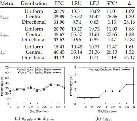
A statistical analysis of these metrics is summarized in Table 5. In order to measure the performance improvement, we calculate an improvement factor over the second best method, denoted by ∆, as follows:

∆= 𝛿_𝑃𝑃𝐶/max⁡{𝛿_𝐿𝑅𝑈, 𝛿_𝐿𝐹𝑈, 𝛿_{𝑆𝑃𝐶∗}} (5)

From these results, we make the following observations:

i. PPC always outperforms LFU, LRU and SPC* under all query distributions. In both uniform and directional scenarios, SPC* works slightly better than LFU

TABLE 5

Average Performance Using Four Cache Mechanisms for Different Query Distributions

Fig.8. PPC performance analysis: effect of grid size. (a) Visited node saving ratio and query time saving ratio, and (b) average deviation percentage.

and LRU. However, under the central distribution, SPC* performs the worst.

ii. PPC receives the highest saving ratio (e.g., δtime =

45.67%) under the central distributed queries, but achieves the best performance improvement (e.g., ∆time = 22.84) from

the second best method in directional distributions.

iii. In directional distribution, we observe a low saving ratio below 2 percent for LFU, LRU and SPC*. This happens because cache-supported systems introduce an additional

cache lookup overhead. When the hit ratio is very low (e.g., 1.19 percent for SPC*), the average response time quickly increases due to the frequent requests to the server. Following a directional distribution, queries are very likely to be a subpart of next queries. Such characteristics fit well with the PPC model but not with the other models.

4.3 Parameter Analysis

PPC successfully reduces the system workload by making full use of the cached results to estimate the shortest path for the new query within a tolerable distance difference. So together with the benefit in terms of visited node saving ratio and query time saving ratio, PPC introduces a service cost due to this distance difference as well. This cost can be measured by the average deviation percentage [2] using Eq. (6), where a smaller value implies a smaller cost:

𝛿_{𝑑𝑖𝑠𝑡} = 𝑝 ∗ − SDP q /SDP(𝑞) × 100% (6)

What follows is a discussion of how the system benefit and the cost are affected by various system parameters such as grid-cell size, cache size, source-destination minimal length and temporal factor.

4.3.1 Effect of Grid-Cell Size

PPC adopts a grid-based solution to detect the potential PPatterns for a new query, so the size of the grid-cell directly impacts the hit ratio and the system performance we examine the system performance in terms of both benefit and cost by varying grid-cell sizes from 1 to 5 km. The results are shown in Figs. 8a and 8b, respectively. The x-axis indicates the grid size and the y-x-axis indicates the metric values as a percentage.

From these figures, we find that the system obtains higher visited node saving ratios and query time saving ratios as the grid size increases. However, the average deviation percentage increases at the same time. By increasing

(8)

4454

the grid size, more cached paths are retrieved as a cache hit which thus prevent sending a complete new query to the server. However, it may retrieve paths that are less relevant so the average deviation percentage increases as well. In a real system, by adjusting the grid-cell size, we can keep a satisfactory balance between the benefit and cost empirically.

4.3.2 Effect of Cache Size

The size of a cache directly determines the maximal number of paths a system can maintain. In this section, we measure the system performance by varying cache sizes with the results shown in Fig. 9. The x-axis is the cache size in terms of the total number of nodes a system can save. We vary it from 1k to 10k nodes with an incremental step of 1k. The y-axis indicates the metric values.

We observe that as cache size increases, the system saves more visited nodes and query time, but with a larger deviation percentage. This is because a bigger cache can potentially maintain more paths and thus increases the opportunity of a cache hit. However it may also introduce a less relevant path. We can choose a proper cache size to avoid unsatisfactory deviation while still saving query time.

4.3.3 Effect of Source-Destination Minimal Length

The minimal source and destination node distance (i.e.,

Dl ¼ =|s0, t0|) in the PPatterns detection algorithm

(Algorithm 1) is another tunable factor. Fig. 10 illustrates the system performance with different distance values. By increasing this distance threshold, the deviation percentage reduces as expected because the coherency property indicates that queries are more likely to share sub paths when the source node is distant from the end node. However, the visited node saving ratio and query time saving ratio decrease because it takes more space to store a longer path therefore, the total number of paths retained in

Fig.10. PPC performance analysis: effect of minimal source-destination distance. (a) Visited node saving ratio and query time saving ratio, and (b) average deviation percentage.

Fig.11. PPC performance analysis: effect of temporal factor. (a) Visited node saving ratio and query time saving ratio, and (b) average deviation percentage.

cache reduces, with the probability of a cache hit consequently decreasing.

4.3.4 Effect of the Temporal Factor

Lastly, we investigate the system performance as time passes. We consecutively insert into the system 50 query groups, each with 100 queries, and observe the average saving ratio and deviation percentage for each group. The statistics are illustrated in Fig. 11. The x-axis indicates the group ID from 1 to 50 and the y-axis indicates the value of different evaluation metrics. As shown, these three ratios are continuously changing as time passes. However, such variation remains steady, which implies that our system robustly and efficiently plans the path for a new query.

V. CONCLUSION

(9)

4455

VI. REFERENCES

[1] Ying Zhang, Member, IEEE, Yu-Ling Hsueh, Member, IEEE, Wang-Chien Lee, Member, IEEE, and Yi-Hao Jhang, “Efficient Cache-Supported Path Planning on Roads”, IEEE Transactions on Knowledge and Data Engineering, Vol. 28, No. 4, April 2016.

[2] H. Mahmud, A. M. Amin, M. E. Ali, and T. Hashem, “Shared execution of path queries on road networks,” Clinical Orthopaedics Related Res., vol. abs/1210.6746, 2012.

[3] L. Zammit, M. Attard, and K. Scerri, “Bayesian hierarchical modelling of traffic flow - With application to Malta’s road network,” in Proc. Int. IEEE Conf. Intell. Transp. Syst., 2013, pp. 1376–1381.

[4] S. Jung and S. Pramanik, “An efficient path computation model for hierarchically structured topographical road maps,” IEEE Trans. Knowl. Data Eng., vol. 14, no. 5, pp. 1029–1046, Sep. 2002.

[5] E. W. Dijkstra, “A note on two problems in connation with graphs,” Num. Math., vol. 1, no. 1, pp. 269–271, 1959.

[6] U. Zwick, “Exact and approximate distances in graphs – a survey,” in Proc. 9th Annu. Eur. Symp. Algorithms, 2001, vol. 2161, pp. 33–48.

[7] A. V. Goldberg and C. Silverstein, “Implementations of Dijkstra’s algorithm based on multi-level buckets,” Network Optimization, vol. 450, pp. 292–327, 1997.

[8] P. Hart, N. Nilsson, and B. Raphael, “A formal basis for the heuristic determination of minimum cost paths,” IEEE Trans. Syst. Sci. Cybern., vol. SSC-4, no. 2, pp. 100–107, Jul. 1968.

[9] A. V. Goldberg and C. Harrelson, “Computing the shortest path: A search meets graph theory,” in Proc. ACM Symp. Discr. Algorithms, 2005, pp. 156–165.

[10] R. Gutman, “Reach-based routing: A new approach to shortest path algorithms optimized for road networks,” in Proc. Workshop Algorithm Eng. Experiments, 2004, pp. 100–111.

[11] A. V. Goldberg, H. Kaplan, and R. F. Werneck, “Reach for A*: Efficient point-to-point shortest path algorithms,” in Proc. Workshop Algorithm Eng. Experiments, 2006, pp. 129–143.