Algorithms for designing filters for optical pattern recognition

A lgorith m s for designing filters

for op tical p attern recognition

E pam inondas Stam os

A thesis subm itted for the degree of

D o cto r o f P h ilosop h y

of the

U n iv ersity o f London.

D epartm ent of Electronic & Electrical Engineering University College London

ProQ uest Number: U 6 4 2593

All rights reserved

INFORMATION TO ALL U SE R S

The quality of this reproduction is d ep en d en t upon the quality of the copy subm itted.

In the unlikely even t that the author did not sen d a com plete manuscript

and there are m issing p a g e s, th e se will be noted. Also, if material had to be rem oved,

a note will indicate the deletion.

uest.

ProQ uest U 6 42593

Published by ProQ uest LLC(2015). Copyright of the Dissertation is held by the Author.

All rights reserved.

This work is protected against unauthorized copying under Title 17, United S ta tes C ode.

Microform Edition © ProQ uest LLC.

ProQ uest LLC

789 East E isenhow er Parkway

P.O. Box 1346

A cknow ledgm ents

My PhD was a long engagement which lasted several years. D uring this period, m any people have helped me in one way or another. I feel very grateful tow ards three people in particular, w ithout whose help and support it would have been impossible for me to do this PhD . My parents, G iannis Stam os and M aria Stam ou and my supervisor David R. Selviah. I feel gratitu d e tow ards my parents for the psychological support they gave me during the project and for th eir crucial financial support, since this PhD was not funded in any other way. A nd I am very grateful to my supervisor for his continuous support and guidance, for his relentless effort to teach me as m any things as possible and for his very long patience to explain to me everything th a t was necessary for my progress and to endure my m istakes and inefficiencies. I th an k them all very much.

D uring my tim e here in UCL I have been a m em ber of th e O ptical Systems and Devices group. All of the other members of the group have been very helpful. I particularly wish to th an k Dr Lawrence C om m ander for spending long hours from his own PhD to be my advisor and my “assistant” . M any th an k s to R obin K ilpatrick, M ark G ardner, K eith Forward and to th e newer mem bers of th e group. Sue Blakeney and Hui-Fang Deng, for sharing th eir com puter program s and th eir knowledge w ith me and for the interesting discussions we have had. I would also like to th an k D r Sally Day and Dr Anibal Fernandez for th eir valuable contribu­ tions and comments during th e group meetings we have held. Laki P anteli for his help and support in the first years of my stay in England. I am also grateful to Dr Tim York for his valuable advice during the first years of my PhD .

A bstract

C ontents

1 In tro d u ctio n 21

2 O p tical inner product correlator fundam entals 25

2.1 In tr o d u c tio n ... 25

2.2 O ptical Fourier transform ... 26

2.3 O ptical C o r r e la to r s ... 26

2.3.1 4-f C o r r e l a to r ... 27

2.3.2 Joint-transform c o r r e l a t o r ... 28

2.4 O ptical M atched f i l t e r s ... 30

2.5 P ractical correlator im plem entations ... 30

2.6 Perform ance m e a s u r e s ... 31

2.7 C o n c lu s io n s ... 32

3 R ev iew o f spatial filter design algorithm s for o p tica l correlators 33 3.1 I n tr o d u c tio n ... 33

3.2 T he G ram -Schm idt orthogonalisation p r o c e d u r e ... 34

3.3 Linear C om bination F ilte r s ... 34

3.4 Synthetic D iscrim inant F u n c ti o n s ... 37

3.4.1 M inimum Variance Synthetic D iscrim inant Function . . . . 39

3.4.2 M inimum Average C orrelation Energy f i l t e r s ... 41

3.4.3 M ICE and MINACE filte rs ... 43

3.5 Phase-O nly F i l t e r s ... 44

3.6 O ptim al Trade-off F i l t e r s ... 44

3.7 Discussion and s u m m a r y ... 45

4 N eu ral networks: P ercep tron s and learning algorith m s 51 4.1 In tr o d u c tio n ... 51

4.2 T he P e r c e p t r o n ... 52

C O N TE N TS

4.3 M ultilayer Feed-forward N e tw o rk s ... 55

4.3.1 The B ack-Propagation learning algorithm ... 56

4.4 S u m m a r y ... 61

5 Sim ilarity Suppression filter design algorith m 62 5.1 In tr o d u c tio n ... 62

5.2 Derivation of th e sim ilarity suppression a l g o r i t h m ... 63

5.2.1 Development of the sim ilarity suppression orthogonalisation a l g o r i t h m ... 63

5.2.2 Development of the sim ilarity suppression cross -orthogonalisation a l g o r i t h m ... 66

5.2.3 Advanced algorithm w ith improved convergence param eters ... 68

5.3 Analysis of th e norm alisation s t e p ... 70

5.4 Com parison w ith other filter design a lg o r ith m s ... 73

5.4.1 Com parison of the G ram -Schm idt orthogonalisation proce­ dure w ith the sim ilarity suppression orthogonalisation algo­ rith m ... 73

5.4.2 The relationship between the SS cross orthogonalisation al­ gorithm and Caulfield’s and M aloney’s Linear C om bination F i l t e r s ... 75

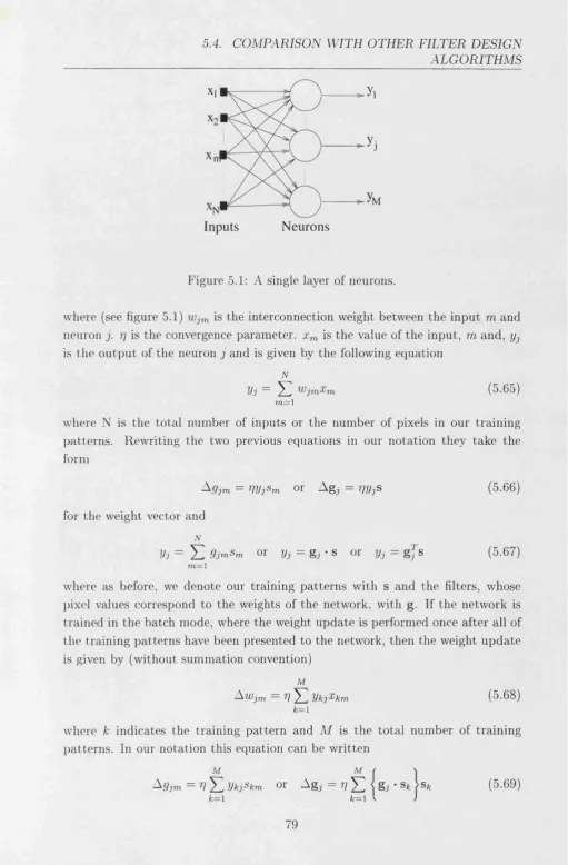
5.4.3 Equivalence between a bank of correlators and a single layer of n e u r o n s ... 78

5.4.4 Com parison of the sim ilarity suppression algorithm w ith the unsupervised Hebbian learning l a w ... 79

5.5 Extension of th e Sim ilarity Suppression algorithm to tra in two or more consecutive banks of c o r r e la to r s ... 82

5.6 Discussion and c o n c lu sio n s... 86

6 C om p u ter sim u lation s o f th e S im ilarity S u p pression a lgorith m 88 6.1 In tr o d u c tio n ... 88

6.2 Convergence S im u la tio n s ... 89

6.2.1 Perform ance M e a s u r e s ... 89

6.2.2 Binary, bipolar p a t t e r n s ... 90

6.2.3 M agnitudes of normalised and un-norm alised filters . . . . 92

6.2.4 Peak-to-C orrelation Energy of the correlations between the training p attern s and the train ed and untrained filters . . 96

C O N T E N T S

6.3 Probability of discrim ination and dynam ic r a n g e ... 101

6.4 Com parison between the filters produced w ith th e SS algorithm and th e linear com bination f i l t e r s ... 104

6.5 O ptim isation of num ber of iterations for the sim ilarity suppression a l g o r i t h m ... 108

6.6 C o n c lu s io n s ... 120

7 Feature E n hancem ent and S im ilarity Suppression filter d esign algorith m 123 7.1 I n tr o d u c tio n ... 123

7.2 D erivation of th e Feature Enhancem ent and Sim ilarity Suppression A lg o r it h m ... 123

7.2.1 Basic a lg o r ith m ... 124

7.2.2 Advanced algorithm w ith improved convergence param eters ... 129

7.3 Com parison of the FESS algorithm w ith relevant filter design and neural network training a l g o r i t h m s ... 130

7.3.1 Com parison of the FESS algorithm w ith the Sim ilarity Suppression A l g o r it h m ... 130

7.3.2 Com parison of the FESS algorithm w ith Synthetic D iscrim ­ inant F u n c tio n s ... 132

7.3.3 Com parison of th e FESS algorithm w ith th e supervised Heb­ bian l a w ... 134

7.4 Extension of the FESS algorithm to two or more consecutive banks of correlators ... 135

7.5 Discussion and c o n c lu sio n s... 137

8 C om p u ter sim ulations o f th e FESS algorith m 140 8.1 I n tr o d u c tio n ... 140

8.2 C om puter S im u la tio n s ... 140

8.2.1 Training set description ... 141

8.2.2 T r a in i n g ... 145

8.2.3 Convergence s p e e d ... 152

8.2.4 Peak to C orrelation Energy (PCE) of correlations between the initial p attern s and the final, train ed class filters . . . 156

8.3 Probability of recognition and dynam ic range ... 160

8.4 C o n c lu s io n s ... 165

C O N TE N TS

9.2 G eneral ach iev em en ts... 167

9.3 Specific a ch ie v e m e n ts... 169

9.4 F uture w o r k ... 172

A p p en d ix A M athem atical definitions 182 A .l Expected value - variance - stan d ard d e v ia tio n ... 182

A .2 C orrelation and covariance m a tr ic e s ... 182

A .3 Fourier tr a n s f o r m ... 183

A .4 Convolution and c o r r e la tio n ... 184

A .5 Inner and outer p r o d u c ts ... 185

A p p en d ix B M agnitudes of th e un-norm alised filters 186 B .l Analysis for the SS a l g o r i t h m ... 188

B.2 Analysis for the FESS a lg o rith m ... 189

A p p en d ix C Training set 191 C .l Training set for the FESS a lg o rith m ... 191

A p p e n d ix D

List o f Figures

2.1 4-f correlator after Collings 1987 [ 1 ] ... 27

2.2 Joint transform correlator after Collings 1987 [ 1 ] ... 28

2.3 O u tp u t of th e joint transform correlator after Collings 1987 [1] . . 29

3.1 Spectral power distribution of an in p u t p a tte rn ... 47

3.2 Inverse filter for the gaussian distribution of figure 3 . 1 ... 48

3.3 A bandpass filter for multiclass p a tte rn r e c o g n i t i o n ... 48

3.4 Effect of th e MACE and MINACE preprocessors on the signal. G raph adapted from [2 ]... 49

4.1 A single layer perceptron w ith only one n e u r o n ... 53

4.2 An example of two linearly separable classes in 2-D space... 53

4.3 A hard lim iter activation f u n c t io n ... 54

4.4 A M ultilayer Perceptron w ith 1 hidden l a y e r ... 56

4.5 Signal-flow graph highlighting the details of o u tp u t neuron k and hidden neuron j, adapted from Haykin (1994) [3 ] ... 57

5.1 A single layer of neurons... 80

5.2 Two cascaded banks of correlators... 83

6.1 Cross-inner product m atrix before th e training. T he graph is shown w ith the X and y axes reversed for clarity... 91

6.2 Total energy index... 91

6.3 Absolute average values of th e 3 largest inner products as a function of iteration num ber for various values of th e convergence factor, /?. 92 6.4 Cross-inner product m atrix after 1500 iterations for a convergence factor of ^ = 6. The graph is shown w ith th e x and y axes reversed. 93 6.5 Unnormalised m agnitudes of some of the filters as a function of th e num ber of ite ra tio n s... 94

L IS T OF FIG U RES

6.7 C ross-inner p ro d u ct m atrix after 1500 iterations w ithout norm ali­ sation for a convergence factor of /? = 6. The graph is shown w ith th e X and y axes reversed for clarity... 95 6.8 N orm alised m agnitudes of some of th e filters as a function of th e

num ber of ite ra tio n s... 96 6.9 C orrelation plane intensity for auto-correlation of p a tte rn 1 and

correlation between p a tte rn 1 and filter 1 ... 97 6.10 C orrelation plane intensity for correlations between p a tte rn 1 and

p a tte rn 2 and between p a tte rn 1 and filter 2... 98 6.11 C orrelation plane intensity for correlations between p a tte rn 7 and

p a tte rn 1 and between p a tte rn 7 and filter 1... 98 6.12 T raining set consisting of ten people’s faces... 100 6.13 V ector-inner pro d u ct m atrix before the train in g ... 100 6.14 Cross-inner pro d uct m atrix after 2000 iterations for a convergence

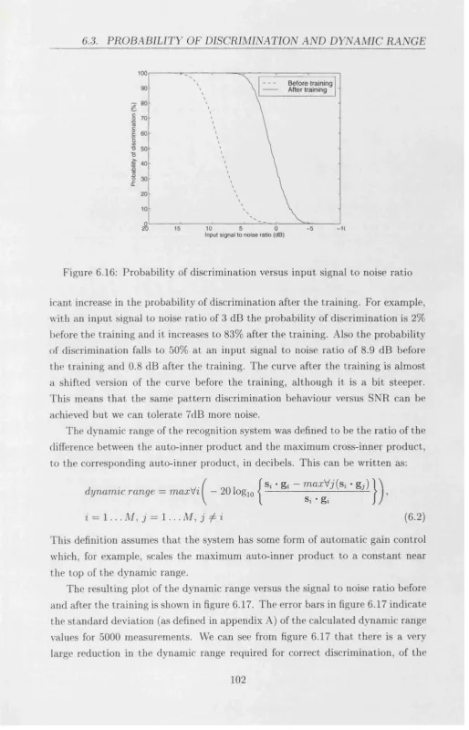
factor of ^ = 0.65... 101 6.15 F inal filters for th e faces s e t... 102 6.16 P ro b ab ility of discrim ination versus input signal to noise ratio . . 103 6.17 D ynam ic range of the recognition system as a function of the signal

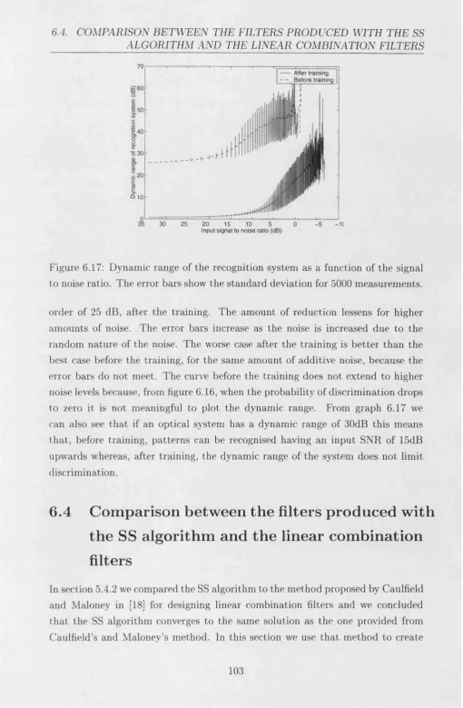
to noise ratio. The error bars show th e stan d ard deviation for 5000 m easurem ents... 104 6.18 C ross-inner prod u ct m atrix between th e in p u t p a tte rn s and th e

filters created using equation 5.55. The graph is shown w ith th e x and y axes reversed for clarity... 105 6.19 Pixel values of th e two versions of filter 2 ... 106 6.20 Differences between pixel values of th e two versions of filter 2 . . . 106 6.21 P ro b ab ility of discrim ination versus input signal to noise ratio . . 107 6.22 D ynam ic range of the recognition system as a function of the signal

to noise ra tio ... 108 6.23 P ro b ab ility of discrim ination versus num ber of ite ra tio n s... 109 6.24 D ynam ic range of the recognition system versus num ber of iterations. 109 6.25 P ro b ab ility of discrim ination versus num ber of iteratio n s for the

first 10 ite ra tio n s... 110 6.26 D ynam ic range of th e recognition system versus num ber of itera­

tions for the first 10 iteratio n s... I l l 6.27 P ro b ab ility of discrim ination as a function of th e signal to noise ratio. I l l 6.28 P rob ab ility of discrim ination difference as a function of the signal

to noise ra tio ... 112 6.29 Pixel values of p a tte rn 2 and filter 2 in th e first 4 and the final

L IS T OF FIG U RES

6.30 Differences between pixel values of th e second filter in various ite r­ atio n s... 114 6.31 C ross-inner product m atrix before the training, in th e first 4 and

in th e final iteration. T he m atrix is depicted from th e side. C.i.p.: C ross-inner p ro d u c t... 116 6.32 D ynam ic range of the recognition system as a function of th e signal

to noise ra tio ... 117 6.33 C orrelation plane intensity for correlation between p a tte rn 1 and

filter 1 after 1500 and after 2 iteratio n s... 118 6.34 C orrelation plane intensity for correlations between p a tte rn 1 and

filter 2 after 1500 and after 2 iteratio n s... 118 6.35 C orrelation plane intensity for correlations between p a tte rn 7 and

filter 1 after 1500 and after 2 iteratio n s... 119

7.1 A single layer of neurons... 134 7.2 Two cascaded banks of correlators... 136

8.1 A sam ple of th e train in g set, which consists of six pictures of each person. O nly three examples of each subject are shown in th is figure. 142 8.2 Cross-inner product m atrix for th e m onopolar p a tte rn s before th e

training. The filters are initially equal to the first p a tte rn of each of th e classes... 143 8.3 F irst and sixth row of th e initial cross-inner pro d u ct m a trix of th e

m onopolar p a tte rn s... 144 8.4 F irst and sixth row of the initial cross-inner pro d u ct m atrix of th e

b ipolar p a tte rn s ... 144 8.5 F irst and sixth row of the final cross-inner p ro d u ct m atrix of th e

m onopolar p attern s after the training w ith th e FESS algorithm . T he initial filters were equal to th e first example of th e correspond­ ing classes... 146 8.6 F irst and sixth row of the final cross-inner p ro d u ct m atrix of th e

m onopolar pattern s after th e training w ith th e FESS algorithm . T he initial filters where equal to the m ean of all of th e exam ples of th e corresponding classes... 147 8.7 F irst and sixth row of th e final cross-inner p ro d u ct m atrix of th e

L IS T OF FIGURES

.8 F irst and sixth row of the final cross-inner prod u ct m atrix of th e bipolar p attern s after the training w ith th e FESS algorithm . The initial filters where equal to the first exam ple of th e corresponding classes... 148 .9 F irst and sixth row of the final cross-inner pro d u ct m atrix of th e

bipolar p attern s after the training w ith th e FESS algorithm . The in itial filters where equal to the mean of all of th e examples of th e corresponding classes... 149 .10 F irst and sixth row of the final cross-inner product m atrix of the

bipolar p attern s after the training w ith the FESS algorithm . The initial filters where random ... 150 .11 Final filters for th e first five subjects, for m onopolar and bipo­

lar p attern s and for all three initial filter values. Column : m onopolar p attern s, initial filters equal to one p attern . 2"^ Col­ um n : m onopolar pattern s, initial filters equal to th e mean of th e p attern s. 3’’^ Column : m onopolar p attern s, random initial filters. 4*^ Colum n : bipolar p attern s, initial filters equal to one p attern . 5*^ Colum n : bipolar pattern s, initial filters equal to the mean of th e p attern s. 6*^ Column : bipolar p attern s, random initial values. 153 .12 Final filters for th e last five subjects, for m onopolar and bipolar p a t­

tern s and for all three initial filter values. 1®^ Colum n : m onopolar p attern s, initial filters equal to one p attern . 2^^ Column : m onopo­ lar p attern s, initial filters equal to th e m ean of the p attern s. 3’’'^ Colum n : m onopolar p attern s, random initial filters. 4*^ Column : bipolar p attern s, initial filters equal to one p a tte rn . 5*^ Column : bipolar p attern s, initial filters equal to the m ean of the p attern s. 6^^ Colum n : bipolar pattern s, random in itial values... 154 .13 Energy ratio for the FESS algorithm p lo tted against num ber of

train in g iterations for the m onopolar p a tte rn s... 155 .14 Energy ratio for th e FESS algorithm plotted against num ber of

train in g iterations for the bipolar p a tte rn s... 155 .15 C orrelation plane intensity for correlations between a photo of the

L IS T OF FIGURES

8.16 C orrelation plane intensity for correlations between a photo of the sixth subject and the untrained (a) and the trained (b) filter for the sixth subject using the m onopolar p attern s. F ilter gg was initially equal to th e m ean of all of the training p a tte rn s in th e 6*^ class. C orrelation peak location: (6 5 ,6 5 )... 157 8.17 C orrelation plane intensity for correlations between th e sixth sub­

ject and th e untrained (a) and the trained (b) filter for th e first subject using the bipolar patterns. The train ed filter was initially equal to the mean of the training p attern s it represents. C orrelation

peak location: (65,65) 158

8.18 C orrelation plane intensity for correlations between a photo of the sixth subject and the untrained (a) and the train ed (b) filter for th e sixth subject using the bipolar patterns. Before th e training, gg was equal to th e mean of all of the training p a tte rn s it represents. C orrelation peak location: (6 5 ,6 5 )... 159 8.19 C orrelation plane intensity for correlations between a photo of the

sixth subject and the trained filter for the first subject (a), and train ed filter for the sixth subject (b) using th e bipolar p a tte rn s and the initially random filters. C orrelation peak location: (65,65) 160 8.20 Convergence index curves of th e SS algorithm w ith and w ithout

th e squared te rm ... 166

9.1 R elationships between our algorithm s, neural network train in g al­ gorithm s and filter design te c h n i q u e s ... 168 9.2 P lan ar correlator. FZP: Fresnel zone plate, MF: M atched filter, IP:

In p u t p a tte rn ... 174 9.3 Disk planar correlator. FZP: Fresnel zone plate, IP: In p u t p a tte rn . 175 C .l The examples th a t were used in the training set for th e first five

people... 192 C.2 The examples th a t were used in th e training set for the last five

people... 193 D.3 F irst three rows of the initial cross-inner product m atrices for m onopo­

lar and bipolar p a tte rn s... 195 D.4 Fourth to sixth rows of the initial cross-inner p ro d uct m atrices for

m onopolar and bipolar p a tte rn s... 196 D.5 Last four rows of th e initial cross-inner product m atrices for m onopo­

lar and bipolar p a tte rn s... 197 D.6 F irst and second rows of the cross-inner product m atrices for m onopo­

L IS T OF FIGURES

D.7 T h ird and fourth rows of the cross-inner product m atrices for m onopo­ lar and bipolar p attern s and all three initial filter values... 199 D.8 F ifth and sixth rows of the cross-inner product m atrices for m onopo­

lar and bipolar p attern s and all three initial filter values... 200 D.9 Seventh and eighth rows of the cross-inner product m atrices for

m onopolar and bipolar p attern s and all three in itial filter values. . 201 D.IO N inth and te n th rows of the cross-inner product m atrices for monopo­

List o f Tables

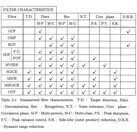
3.1 Sum m arised filter characteristics. T.D . : Target detection, Discr. : D iscrim ination, Rec. : Recognition, N.T. : Noise tolerance, Corr. plane : C orrelation plane, M -P : M ulti-pattern, M-C : M ulti-class, P.S. : Peak sharpness, P.V. : Peak variance control, S.R. : Side-lobe (outer product) reduction, D.R.R. : Dynam ic range reduction. . . 46

6.1 N um ber of pixels differing in th e training s e t... 90

6.2 Com parison between the filters produced w ith th e SS algorithm af­ ter 2 iterations and the LCFs. SS 2 i.: SS algorithm 2 iterations, H.I.N.: High input noise, L.I.N.: Low input noise, H.D.R.: High re­ quired dynam ic range, L.D.R.: Low required dynam ic range, Loc.: Location detection. High Disc.: High D iscrim ination ability. High Rec.: High recognition a b i l i t y ... 120

8.1 Mean value and stan d ard deviation of th e auto- and cross-inner products for the m onopolar patterns. The last column in th e table shows the ratio of the mean of the auto-inner products over the mean of the cross-inner p ro d u cts... 150

8.2 Mean value and stan dard deviation of the auto- and cross-inner products for the bipolar patterns. The last colum n in the table shows the ratio of the m ean of the auto-inner products over the mean of the cross-inner p ro d u cts... 151

8.3 Probability of recognition and dynam ic range using th e train in g set. 161 8.4 Probability of recognition, false positives, false negatives and dy­

L IS T OF TAB LES

N o ta tio n

j3 : Convergence param eter

r] : Convergence param eter

r)H : Horner efficiency

Q : Neuron threshold A : Positive real num ber

^ : Uniform background image

E : Noise covariance m atrix

cr^ : Variance

<f)[') : Neuron activation function

a : Solution vector for synthetic discrim inant functions

a : Coefficient for calculating equal correlation peak filters

b : Coefficient for calculating equal correlation peak filters

C : M X M m atrix whose elements are th e coefficients C C : Coefficient for calculating linear com bination filters c : Coefficient for calculating equal correlation peak filters

d : Desired neuron or correlator o u tp u t value

D : How often (iterations) the addition equation of the FESS algorithm is applied

D : N X N diagonal m atrix

d : Vector w ith desired correlation o u tp u ts

E {-}: Expected value

Eave : Average correlation plane energy e : Neuron o u tp u t error

F : C orrelation response f : In p u t image

G : M X 1 vector whose elements are th e filters g

g : Unnorm alised correlation filter

0)g ; g filter in the jth bank of cascaded banks of correlators g(^) : g filter a t the ith application of th e SS or FESS algorithm

K : Num ber of classes

L j : N um ber of training p attern s in th e jth class

M : T otal num ber of p attern s in the train ing set

N : Size (in pixels) of training p attern s and filters

n : Noise vector

O : Total num ber of neurons in the network

P : Power of normalised training p attern s R : Vector inner product m atrix

r : Value of inner product of two p attern s S : M atrix whose lines are the training vectors s

s : Training p a tte rn

s : Mean of training p attern s s

T : N X N diagonal m atrix

t : Neuron o u tp u t targ et value

u : P a tte rn orthogonal to the other p attern s in its set

Û : U nnorm alised orthogonal p attern

V : Set of N real numbers

V : Neuron net internal activity level

w : Neuron weight

X : Neuron input

y ; Neuron outpu t

z : Complex num ber of m odulus 1

z : Vector of real numbers

★ : Symbol denoting convolution

(g) : Symbol denoting correlation

A b b reviation s

B P O F : B inary Phase Only Filter

B P O SDF : B inary Phase Only Synthetic D iscrim inant Function

CCD : Charge Coupled Device

E C P : Equal C orrelation Peak

FESS : Feature Enhancem ent and Sim ilarity Suppression

fSDF : filter Synthetic D iscrim inant Function

F T : Fourier Transform

G M F : Generalised M atched Filter

JT C : Joint Transform C orrelator

LCF : Linear C om bination Filter

LDF : Linear D iscrim inant Function

MACE : M inimum Average C orrelation Energy

M HP : Modified Hyper Plane

M ICE : M inimum C orrelation Energy

M INACE : M inimum Noise And C orrelation Energy

M LP : M ulti Layer Perceptron

M OF : M utually O rthogonal Filter

MOSLM : M agneto Optic Spatial Light M odulator

M VSDF : M inimum Variance Synthetic D iscrim inant Function

occ

P C E : Peak to C orrelation Energy

P O E ; Probability Of E rror

PO E : Phase Only Filter

P C SDF : Phase Only Synthetic D iscrim inant Function

SDF : Synthetic D iscrim inant Function

SLM : Spatial Light M odulator

SNR : Signal to Noise R atio

C hapter 1

In trod u ction

In this thesis we develop two algorithm s for designing filters for optical p a tte rn recognition. We investigate their perform ance using theoretical calculations and com puter sim ulations. In addition, we compare our algorithm s to relevant exist­ ing techniques for designing filters for optical p a tte rn recognition and to neural network training algorithm s.

The original aim of this project was to develop an optically im plem entable algorithm for training neural networks. This was based on an initial version of one of our algorithm s for designing filters for optical p a tte rn recognition, which was based on the G ram -Schm idt orthogonalisation procedure, and on th e already known relationship between neural networks and optical correlators [4]. O ur in itial aim s were to further dem onstrate, develop and improve our algorithm and to assess its lim itations. To investigate w hether it could be used to tra in neural networks and its relationship to other neural network training algorithm s. A nd to design and build an optical system which would im plem ent our train in g algorithm .

Various reasons, m ost im p o rtan t among which being th e interesting results we obtained from our com puter simulations and th e theoretical com parisons w ith other training algorithm s and filter design techniques, led us to emphasise th e theoretical p a rt of the project. In addition, we focused on th e optical filter design side of the project and not on the neural network side, because of the currently higher interest in optical filters ra th e r th an optical neural networks. In th e fol­ lowing paragraphs we present some background inform ation on the relevant fields, nam ely optical p a tte rn recognition and neural networks, which will help us place our work in the context of related research.

Chapterl. Introduction

have the advantage th a t they are very fast com pared to com puters. This speed advantage is a consequence of the inherent parallelism of optics and th e speed of light. Moreover, there are optical correlators, which can correlate m any im ­ ages w ith one in parallel [8]. The m ost im p o rtan t com ponent of any recognition system based on a correlation is th e tem plate, or filter, w ith which the in p u t p a t­ tern is com pared. This filter depends on the correlator im plem entation (optical, electronic, hybrid etc.). Some optical correlators use filters in the space dom ain [9, 10] and others in the Fourier dom ain [5]. Furtherm ore, th e filters depend on th e p articu lar task a t hand. Some system s’ prim ary aim is to detect th e pres­ ence of an object in a noisy background. For example, m atched filters, which are th e complex conjugates of the spectrum of the original p attern s, are optim al for detecting signals in white, Gaussian noise [11]. The aim of other system s is to recognize the presence of any one of several p attern s in th e input, for example, SD F filters [12, 13, 14, 2] and optim al trade-off filters [15, 16, 17]. O ther system s aim to distinguish between very sim ilar objects, for example, m utually orthogonal filters [18]. All of these are not completely different tasks, on the contrary, they are inter-related and many filters are designed w ith all of these aims in mind. M ost of th e previously mentioned filters are linear com binations of training p a tte rn s and their design m ethods are based on solving a set of sim ultaneous equations, to calculate an array of coefficients. These coefficients can th en be used to lin­ early combine the training patterns, to create the filters in such a way th a t th eir correlations w ith the input p attern s yield the desired o u tp u t values.

N eural networks [3] are simplified models of the hum an brain. They consist of m any simple processing units called neurons. These neurons are interconnected w ith connections of different strengths. The strengths of these interconnections are called weights and determ ine the behaviour of the network. The m ethods for modifying these weights are called training algorithm s. Most of th em are iterative and they apply a m athem atical rule to modify th e netw ork’s weights, usually based on a num ber of training examples. Sometimes, these m athem atical rules are ra th e r complicated. In addition, many iterations and a large num ber of tra in in g examples may be necessary for the network to yield th e desired o utputs. Therefore, th e training of a neural network is often a tim e consuming process. Furtherm ore, as th e desired network behaviour may change w ith tim e, the network may need to be retrained.

C hapterl. Introduction

cess of train in g neural networks. D uring the project, we decided not to work on th e practical optical system to im plem ent our train in g algorithm , b u t instead to concentrate on the algorithm development. Also we shifted the em phasis from neural networks to optical filters and we investigated th e relationship between neural netw ork training algorithm s and optical filter design techniques using our algorithm s as an interm ediate step for the comparisons, which led to some very interesting results. So our revised, final aims are sum m arised below:

1. To fu rth er dem onstrate, develop and improve our algorithm .

2. To assess its lim itations.

3. To develop, dem onstrate, and assess the lim itations of a second algorithm which addresses the problem of m ulti-class p a tte rn recognition.

4. To investigate the relationship between our algorithm s and some neural network training algorithm s.

5. To com pare our algorithm s to some relevant optical filter design techniques.

Chapterl. Introduction

C hapter 2

O ptical inner product correlator

fundam entals

2.1

Introduction

2.2. O PTIC AL FO U RIER T R A N SF O R M

2.2

Optical Fourier transform

According to the Fraunhofer approximation [19], when an ap ertu re is illum inated w ith coherent light the far-held diffraction p a tte rn is th e Fourier transform of th e complex ap ertu re distribution, as shown in equation 2.1

J l dÇdr, (2.1)

— OO

where, A is the wavelength of the light, z is th e distance from th e ap ertu re and

k = ^ is the propagation number, the m agnitude of th e propagation vector, k. If a lens is inserted im m ediately after the diffracting aperture, th en it focuses the far-held p a tte rn onto the focal plane. The am plitude d istrib u tio n a t th e focal plane of the lens is

E {x , y) = ^

JJ

— OO

where th e constant phase factor is ignored and / denotes th e focal length of the lens. This equation is almost identical to the 2-dimensional Fourier transform equation shown in equation 2.3. The only difference between the two equations is

j k ( x ^ + y ^ )

the quadratic phase factor term e 2/

F { x , y ) = [ (2.3)

J x J y

It has been shown [19] th a t when the diffracting ap ertu re is located a t th e front focal plane of the lens, then this quadratic phase factor is removed and an exact Fourier transform relationship exists between th e front and back focal planes. As far as the inverse Fourier transform is concerned, which is shown in equation 2.4,

J { x , y ) =

[ f

J x J y

th is can be obtained by performing a forward Fourier transform optically and then calculating th e m irror image along th e x and the y axes of the o u tp u t.

2.3

O ptical Correlators

By making use of the convolution theorem^, it is possible to com pute th e con­ volution of two functions much faster by perform ing two F F T s, one inverse F F T

2.3. O PTIC AL C O R R E LA TO R S

Input plane

SLM

C oh eren t input ligh t

Fourier plane

SLM PL

Output/correlation plane

Figure 2.1: 4-f correlator after Collings 1987 [1]

and N m ultiplications instead of 2 N ‘^ m ultiplications th a t would be necessary for the convolution [20]. Even then, however, the convolution or correlation of two functions can be a tim e consuming calculation, and dedicated chips have been m anufactured to perform them [21]. O ptical convolution or correlation is very fast, because an aperture can perform a Fourier transform w ith a lens bringing it into the near field and giving it the correct phase. Also the m ultiplication is very easily im plem ented optically [22], by, for example, illum inating a sandwich of the two images. The speed of the optical im plem entation of the correlation has led to the design of several kinds of optical correlators.

2 .3 .1

4 - f C o rrela to r

A very simple optical correlator is shown in figure 2.1. It is called the 4~f corre­ lator or th e frequency plane correlator. The first lens is perform ing th e Fourier transform of the input function, i{x, y), which is displayed on the first spatial light m odulator (SLM) and is illum inated w ith coherent light. The complex conjugate,

F*{u, u), of the Fourier transform of the filter function, f { x , y), is displayed at the back focal plane of the lens using the second SLM. The two Fourier transform s are m ultiplied, the light leaving the second SLM is the product I ( u, v)F*{u, v), and at the back focal plane of the second lens, which is perform ing another Fourier tra n s­ form, the o u tp u t is equal to the cross-correlation of the two functions in the space dom ain [20]. The 4-f correlator uses Fourier dom ain m atched filtering because the Fourier transform of the filter m ust be displayed on the second SLM. Obviously the Fourier transform of any filter is a complex function. The photographic film th a t was initially used for the im plem entation of the 4-f correlator was not

2.3. O PTIC AL C O R R E LA TO R S

Dynam ic holographic recording device BS

Spatial Filter

Input

c p p LI

Photodetector array

D

D

Hologram construction H ologram interogation

laser laser

Figure 2.2: Joint transform correlator after Collings 1987 [1]

inally [23] able to accom m odate complex transm ittances. Vander Lugt^ [5] was the first to propose a m ethod for bypassing the problem by using a holographic filter. To do th a t he recorded the intensity of the interference between the filter

F { u ,v ) and an off-axis reference beam. According to K um ar in [23], ''when this mask is placed in the back focal plane of the first F T lens, the light leaving it has three distinct components [23]: First is the product k I(u ,v )[ A ^ 4- \F {u ,v )\‘^],

where k is a normalising constant and A is the amplitude of the reference beam, and its inverse F T appears centered on the optical axis at the output plane. The second term is k A I{ u , v )F (u , v)e^‘^^, where a is related to the angle of the reference beam. Its inverse F T is the convolution between the filter and the input functions, a,nd it is placed along the x-axis on one side of the origin. The third term is k A I[u ,v)F * {u ,v)e~ ^°‘''^, whose inverse F T produces the desired correlation along the x-axis at the opposite side of the origin.^' Obviously the reference beam angle, a, plays an im portant role to the placement of the correlation a t the o u tp u t plane and a steep enough angle m ust be chosen to ensure good separation between the three terms.

2 .3 .2

J o in t-tr a n sfo r m co r re la to r

The joint transform correlator (JTC ) [9, 10] is based on a different approach, where the prior Fourier transform ation of the filter is not necessary. In the joint

^Vander Lugt used amplitude masks made of photographic film and not SLMs in his imple­

2.3. O PTIC AL C O RR E LA TO R S

Filter

Input _Write

(a) (b)

RF*I

R(IFI+II|)

RFI Read

Figure 2.3: O u tp u t of the joint transform correlator after Collings 1987 [1]

transform correlator, figure 2.2, the input image and the filter are presented at

the input plane of the F T lens (L3) a t the same tim e, and are then bo th Fourier transform ed by the lens. The interference p a tte rn of th eir Fourier transform s is recorded in a real-tim e recording m aterial such as a photorefractive crystal which is a t the back focal plane of the F T lens. The hologram is interrogated w ith a collim ated beam. The o u tp u t beam is sent through a second F T lens and the correlation of the input and the filter p attern s is obtained at the o u tp u t. The reconstructed beam in the JT C consists of three term s (figure 2.3). The on-axis term is the sum of the auto-correlations of the object and the scene, 7 ? (|F p -f 1/|^). The off-axis term s are the term s of interest because they are the cross-correlations of the in p u t and the filter, R F I* and R F * I, where i?, denotes the am plitude of the reference beam. To obtain a convolution, the m irror image of either the filter or the in p u t function m ust be placed at the input of the JT C .

The m ain difference between the JT C and the 4-f correlator is th a t the JT C perform s spatial-dom ain instead of Fourier dom ain filtering. In other words, the filter th a t is placed in the 4-f correlator m ust already be in the Fourier dom ain, while in th e JT C the filter must be in the space domain. The main advantage of the JT C is th a t no great accuracy in the positioning of the input and the filter is required [1]. However, any change in the positioning of the input relative to the filter (or visa versa), will result in the change of the angle 2a between them and hence, the position of the cross-correlation peak at the o u tp u t, as can be seen in figure 2.3. Provided th a t real-tim e devices are available, search routines can be perform ed at the frame rates of the SLMs. In addition, th e JT C can be used for adaptive p a tte rn recognition, where the input signal is continually being com pared to a reference signal which is changing in tim e [23]. However, the optical quality of the in p u t devices, and the FT lens used in the JT C m ust be high.

2.4. O PTIC AL M ATCHED F ILTER S

2.4

O ptical M atched filters

A matched filter is a time-reversed version of th e in pu t signal h{x) = s{—x), where

s{x) is th e in p u t signal. If the input signal is complex and 2D, th en th e tim e reversed complex conjugate of its frequency spectrum , h{x, y) = s*{—x, —y), is its m atched filter. It has been proved th a t m atched filters are optim al for detecting the presence of th e signal s(a;) in a noisy input, when th e noise is w hite w ith a constant power spectral density [11, 23]. This optim ality of th e m atched filters in detecting signals buried in noise is proved because it maximises the o u tp u t Signal- to-Noise R atio (SNR), which leads to a m inim um probability of error [24]. An optical m atched filter can be im plem ented by a hologram containing th e complex conjugate of th e frequency spectrum of the p a tte rn [1], or using an am plitude and

a phase SLM.

2.5

P ractical correlator im plem entations

Purely optical correlators have the advantage of being very fast, operating a t over kHz rates [25, 26], b u t they suffer from several disadvantages such as th e lack of versatility and program m ability, and low accuracy due to th e analogue n atu re of optics and th e low dynam ic range [27]. On the contrary, all of the previously m entioned deficiencies of the optical systems, are strong points of electronic com­ puters. It is no t strange, therefore, th a t many hybrid system s have been developed which combine th e advantages of b o th worlds [16, 28, 29, 30, 31, 32, 33, 34, 35].

In m any cases the in p ut image m ust be correlated w ith a very large num ber of reference images. These reference images can either be stored in a com puter and dow n-loaded to the correlator sequentially, or they can be stored optically. In th a t case th e storage device is p a rt of the correlator. O ptical disks have been successfully used in correlators [36, 37, 38, 39]. A nother solution is the use of photorefractive m aterials, which offer large storage capacity [40], high resolution and real-tim e recording and several correlators have been bu ilt which utilise them [41, 42, 43].

mod-2.6. PE RF O R M A N C E M EA SU RE S

ulators for the d a ta input to the optical p a rt of th e system and CCD cam eras for the correlation readout. Then the com puter makes th e decision based on th e correlation output. In addition, all of the preprocessing of the d a ta before it is down-loaded to the SLM and the post-processing of the correlation o u tp u t is done by th e com puter.

It is ap paren t th a t the SLMs play a very im p o rtan t role in these architectures, since they depend not only on their speed, b u t also on th eir ability to m odulate th e am plitude or th e phase of the passing light, or bo th [50, 51]. There is currently no SLM commercially available, which can sim ultaneously fully m odulate the am plitude and the phase of th e passing light. Therefore, several filters have been designed, which use only a p a rt of the complex plane [16, 52]. In addition, a com bination of two SLMs can be used for sim ultaneous am plitude and phase m odulation [52, 53, 54, 55].

2.6

Perform ance m easures

Several different perform ance measures have been proposed by various authors for th e assessment of the perform ance of optical filters. T he m ost frequently used of these perform ance m etrics were sum m arised in a pap er w ritten by K um ar and H assebrook [56]. Later in the thesis we are going to use some of these perform ance m etrics to assess the perform ance of our filters and to com pare it w ith th e per­ form ance of other filters. Therefore, following the K um ar and Hassebrook paper, we present and explain the following perform ance metrics:

1. Signal-to-Noise R atio

T he Signal-to-Noise R atio (SNR) is defined as th e ratio of th e square of the average m agnitude of th e correlation peak, over the variance of th e m agnitude of the correlation peak:

T he SNR gives us a m easure of how much the correlation peak fluctuates when random noise is added to the in p u t signal. Obviously, it is desirable to keep these fluctuations as small as possible, or in other words to m aximise th e SNR. It is evident from equation 2.5 th a t to calculate th e SNR, one needs to calculate the average and th e variance of th e m agnitude of th e correlation peak. Therefore, m any experim ents w ith different noise sam ples have to be conducted for the SNR to be estim ated.

2.7. CONCLUSIONS

T he Peak-to-C orrelation Energy (PCE) is defined as th e ratio of the square of th e m agnitude of th e correlation peak, over the correlation plane energy:

P C E = (2.6)

t/y

where

/

-O O

T he P C E measures the sharpness of the correlation peak. W hen th e cor­ relation has a sharp high peak and low outer products, th e energy of th e whole correlation Ey will not be much larger th a n th e energy concentrated on th e peak, and the P C E will be large (close to 1). If the correlation peak is no t sharp, or th e outer products are large, then th e PC E will be closer to

0.

3. H orner efficiency

In 1982 Horner [57] introduced the Horner efficiency criterion. The H orner efficiency is the ratio of to tal light energy in th e o u tp u t plane to th e light energy a t the input plane and is described by th e following equation

where f { x ) is the input function, h{x) another function, r}M th e diffraction efficiency of the recording m edium, and the operator 0 indicates correlation.

T he H orner efficiency measures the am ount of light th a t passes through th e system .

2.7

Conclusions

C hapter 3

R ev iew o f spatial filter design

algorithm s for op tical correlators

3.1

Introduction

O ptical p a tte rn recognition is a m ulti-faceted problem. It includes th e detection of objects buried in noise [58, 59, 60, 61], the discrim ination of different objects [62], the recognition of different views of a 2D [63, 64] or 3D [65, 6 6, 67] object

and the discrim ination of them from other views of a different 2D or 3D object [6 8]. Due to th e complexity of these different recognition or discrim ination prob­

lems, researchers have proposed m any different m ethods and algorithm s for the developm ent of the appropriate filter for each case [69]. In this chapter, we review some of the algorithm s proposed in th e literature. O nly a few of these algorithm s, which are the m ost sim ilar to our work and which will be com pared to it in later chapters are presented in detail here. Different authors have used different n o ta­ tion in their publications. For the sake of clarity, we have changed th a t n otatio n where necessary and we have used one set of symbols consistently throughout the chapter.

3.2. T H E G R A M -S C H M ID T O R T H O G O N A L IS A T IO N P R O C E D U R E

to gfc ' Sjfc or in vector notation g^s.

3.2 T he G ram -Schm idt orthogonalisation

procedure

Given a set of vectors Si, 8 2, Sm, in TV dim ensional space R ^ , M < N , th e G ram -

Schm idt O rtho-norm alisation procedure [70] constructs an orthonorm al basis set of vectors spanning the space 5'= span(si, 8 2, (which is the set of all linear

com binations of the vectors 8 1,8 2, 8m)- The algorithm begins by norm alising

th e first vector 8 1,

where || • H2 denotes th e Euclidean norm

N \ 1/2

(3.2)

8 2 is m ade orthogonal to 8 1 and it is norm alised by the following two iterative

steps;

Ufc+l = S/c+i) (3.3)

T hen 8 3 is made orthogonal to 8 1 and 8 2 and norm alised and so on using the

same iterative and norm alising equations. Once k vectors have become orthogonal spanning a subspace Sk C 5 , s^+i is projected onto th e subspace orthogonal to

Sk- Finally, all of the M vectors will be orthogonal, so Sm will be equal to S.

3 . 3

Linear Com bination Filters

3.3. L IN E A R CO M BINATIO N FILTE R S

were mutually orthogonal^ (MO) was proposed by Caulfield and M aloney [18] as a solution to the discrim ination problem. Each of the filters had un it o u tp u t when correlated w ith one of the input p attern s and zero w ith all of the others. The first step of the procedure was to calculate th e vector inner-product m atrix of the train in g p a tte rn s

f 'I'll y 12 • ’ ' I^1m \

^21 'f'22 • • ' T 2 M

\ f ' M l 'f'M2 • • • 'Tm mJ

(3.5)

where Vij = Sj • Sj or in other words each element of th e m atrix was equal to th e inner product between the input p attern s s% and Sj. Caulfield’s and M aloney’s aim when testing p a tte rn for its identity to p a tte rn S)t, was to obtain an o u tp u t, Fife, equal to one i ï i = k and equal to zero l i i ^ k, i.e.,

Fik = Fkk^ik (3.6)

T hey achieved their aim w ith th e second step of the procedure, which was to form linear combinations of the responses r^ . Using these linear com binations the final response when testing p a tte rn s% for its identity to would be

Elk — Tik T ^ 1 OklTii (3.7)

l^k

T he M — 1 %’s for which % ^ A: led to a set of M — 1 sim ultaneous equations w ith M — 1 unknowns, the coefficients Cki- A different set of M — 1 sim ultaneous equations w ith M —1 coefficients had to be solved for each of th e M input p attern s. A fter calculating the coefficients Cki, Caulfield and Maloney used equation 3.7 to see w hether an in p u t p attern , s% was the same as p a tte rn s^. If th e equation o u tp u t was equal to one, then p a tte rn i was the same as p a tte rn k, and if it was equal to zero, then p a tte rn i was different from p a tte rn k. Caulfield’s m ethod does n o t actually produce new filters. R ather, it combines th e inner products between th e train in g p attern s to obtain an o u tp u t which will determ ine w hether an in p u t p a tte rn is th e same as another p attern . However, th eir coefficients can be used to create th e actual filters, which will yield th e desired o utp u ts. Caulfield and M aloney m entioned this in their paper, b u t a t the tim e th a t they wrote it, it was difficult to make these filters.

L ater Caulfield and Haimes [71] proposed a more generalised solution to th e m ulti-class - m ulti-object recognition problem w ith th e Generalised Matched Filter

(G M F). T heir aim was to create filters which would be able to recognise all of the

3.3. L IN E A R CO M BIN ATIO N F ILTER S

p a tte rn s w ithin a class and, in addition, discrim inate between members of different classes. They supposed th a t each in p u t object, s was of size N . For each class of objects they calculated a Linear Discriminant Function (LD F), which they used as the generalised m atched filter. This filter would have a high correlation o u tp u t w ith any p a tte rn th a t belonged to th e class it represented and a low o u tp u t for any p a tte rn which belonged to any of the other classes. The L D F was a real function of th e train in g p a tte rn s

LDFi{s) = V j • s + Qoi = Fi{s) (3.8) where V% = (V i,V2, . . . , was a set of real num bers and Qoi was a real num ber. They chose th e L D F which would have a high o u tp u t w ith the members of th e class it represented and a low o u tp u t w ith all of the other in p u t objects by m axim ising th e equation

E[LD Fi{s € Classi) — LD Fi{s ^ Classi)] (3.9) where E[-] was the expectation operator. In other words L D F i was th a t linear function of s th a t maximised th e probability to distinguish s € ClasSi from s ^

ClasSi. If th e LDFs were normalised, then

E \L D F i{ s G (7/assj)] = 6ij. (3.10) Equations 3.10 and 3.6 show th a t the m utually orthogonal filters are a subset of th e generalized m atched filters, because if each of the classes only consists of one p a tte rn , then equation 3.10 expresses the same condition as equation 3.6.

A filter th a t would have equal correlation o u tp u ts w ith all of the p a tte rn s representing one class in a multi-class recognition problem was proposed by H ester and Casasent [72]. It was called th e Equal Correlation Peak (ECP) filter. F irstly th e G ram -Schm idt procedure was used to orthogonalise th e training images Sj

and to produce a new set of orthogonal vectors th a t formed an orthonorm al basis of the space of the input and training images. T hen th e in pu t images, f, and the training images, s were expanded in this set of orthonorm al vectors Uj

f = ^ ^j'^j (3 11)

j

S = 12 (3-12)

3

and th e input and training images could be represented by th e coefficients Uj and

bj

f = ((%1, <22) • • • ) ®/c) (3.13)

3.4. S Y N T H E T IC D ISC R IM IN A N T FU NCTIO NS

In term s of these expansions the inner product of f and s could be described by

Tfs = f ' S = ' ^ üjbj (3.15)

j

T he objective was to design a filter, g, which would have equal correlation o u tp u ts w ith all of th e inputs, fj, which belong to the same class. Hester and C asasent argued th a t th is filter had to be a specific linear com bination of th e in p u t images, each of which was another linear com bination of th e basis functions u

g = e = T CjU, (3.16)

j j

and th e correlation outp u ts could then be described by

j

So after finding the orthogonal vectors Uj, using th e G ram -Schm idt orthogonali­ sation procedure, and the coefficients bj, using equation 3.12, the objective was to find the coefficients Cj and finally th e filter g for which r in equation 3.17 would yield the correct correlation performance. If one required rgg (equation 3.17) to be equal for all training p attern s s, he could solve the resulting set of equations to obtain the coefficients Cj.

3.4

Synthetic Discrim inant Functions

T he work on linear combinations of training images, i.e. LCFs, EC Ps and GM Fs, was sum m arised by Caulfield [73] and Casasent and K um ar et. al. and it was form ulated as a m atrix /vecto r problem [13, 74]. The solution vectors to th e LC Fs were described by the equation

^ = ^ (3.18)

ai = R di

where R was the M x M correlation (alternatively called vector-inner product) m atrix of the in p u t images and d was the vector w ith th e desired correlation outp u ts. The vector-inner product m atrix R was invertible if and only if the in p u t p attern s were linearly independent [69]. T hen the filters could be obtained using these solution vectors

Si ~ ^ V Q'fcSfc (3.19)

3.4. SY N T H E T IC D ISC R IM IN A N T FU NCTIO NS

where ak are the elements of the solution vector a%. D epending on th e desired correlation o u tp u t vectors, d%, equation 3.18 was equivalent to equation 3.7, if m utually orthogonal filters were required.

Caulfield’s and M aloney’s approach (m utually orthogonal filters) m eant th a t one filter had to be designed for each of the M p attern s th a t one wanted to recog­ nise. Each in p u t p a tte rn had to be correlated w ith all of them . Therefore, M correlations were necessary for correct recognition. Braunecker et. al. [75] sug­ gested th a t M filters were redundant and th a t one only needed to perform a t m ost

L = logg M correlations to correctly recognise M filters. Braunecker’s approach was based on th e fact th a t L = logg M binary digits can form any num ber between 0 and M . For example, to recognise 4 p attern s one needed only two filters, the first of which should yield a high correlation peak only w ith the second and th e fo u rth input p a tte rn and the second filter should produce a high correlation peak only w ith the th ird and the fourth in p u t p attern . B raunecker’s approach could also be applied to m ulti-class p a tte rn recognition. The two previously reviewed m ethods, i.e. linear discrim inant functions and equal correlation peak filters de­ signed one filter for each class. Therefore K , where K is th e num ber of classes one wants to recognise, correlations were necessary for correct recognition of an in p u t p attern . According to Braunecker’s m ethod, only L — logg K correlations are necessary.

Even faster recognition could be achieved if only one filter was designed, which gave the same correlation peak value for all of the p a tte rn s th a t belonged to one class and a different, in intensity, correlation peak value for all of the p a tte rn s th a t belonged to another class and so on. This particu lar linear com bination filter was called a Synthetic Discriminant Function (SDF) [13, 74]. The advantage of SDF was th a t only one correlation would be necessary to recognise any of th e input p attern s. T heir disadvantage was th a t they required th a t th e recognition system h ad a high dynam ic range, because several different correlation peak values had to be correctly identified a t th e o u tp u t plane. A year later, in 1983, the Modified Hyperplane Method (MHP) for more efficient design of Linear C om bination Filters (LCFs) was proposed by K um ar [76]. A system atic procedure for determ ining the o u tp u t correlation values for SDFs, instead of arb itrarily settin g them to 0 and 1, was proposed by Sudharsanan and M ahalanobis et. al. [77]. T he proposed technique provided an optim al selection of th e o u tp u t correlation values in the sense th a t they resulted in a m inim ization of th e probability of error (P C F ) in detection.

3.4. SY N T H E T IC D ISC R IM IN A N T FU NCTIO NS

often th ey gave high correlations w ith false targets. He observed th a t only inten­ sities were detected at the correlation plane, so o u tp u t correlation values could have a rb itra ry phase. He used this additional degree of freedom to reform ulate th e equation describing the SDFs (equation 3.18) in the following m anner

g • Si = ZiXi { l < i < M) (3.20)

where Si,(l < i < M) were the complex images of objects one w anted to recognise T he Ai were given positive numbers and Zi were complex num bers of m odulus 1. E quation 3.20 gave M sim ultaneous equations th a t g had to satisfy and a p articu lar solution to this equation would have th e form

go = ttiSi -|-. . . -f clm^m (3.21)

where Gi . . . a u were a set of complex numbers. These num bers could be found by su b stitu tin g equation 3.21 into 3.20

(S i-S j)(a j) = {ziXi) (3.22)

E quation 3.22 uniquely determ ined the complex num bers Oi if th e images S i . . . Sm

were linearly independent and is identical to th e general SDF solution equation shown in 3.18. K allm an proposed th a t one could m axim ise th e SNR of th e filters by varying th e z* phase values of th e inner products and choosing the approp riate of m any possible solutions to equation 3.20. Using his m ethod, K allm an m anaged to construct filters w ith th eir SNR properties improved by a factor of seven [78].

3 .4 .1

M in im u m V a ria n ce S y n th e tic D is c r im in a n t F u n c tio n

As we saw in th e previous section, SDFs yield one correlation peak w ith a different intensity value for each of the classes to be recognised. As th e num ber of classes increases, th e different values of the correlation peak will be closer to each other, because m ore of them will be needed in an overall lim ited range. This m eans th a t the variance^ of the correlation peak is critical for th e filter’s perform ance. T he

M in im u m Variance Synthetic Discriminant Function (M VSDF) which m inim ised the variance of the correlation peak, which was caused by noise, was introduced by K um ar [14]. K um ar addressed the problem where the in p u t was one of th e train in g images w ith some additive noise. In th a t case the o u tp u t of th e correlation a t th e origin of th e correlation plane would be

y = g+(si -f n) = Ci -f g + n (3.23)

3.4. S Y N T H E T IC D ISC R IM IN A N T FU NCTIO NS

where g denoted th e filter which was designed to satisfy equation 3.18, g+ denoted th e conjugate transpose, s% denoted th e input p a tte rn and n was a zero-mean noise vector w ith a covariance^ m atrix E. The o u tp u t in this case was the desired o u tp u t

Ci plus an undesirable random variable g ^ n . The M VSDF attem p ted to design th e filter g in such a way so th a t the variance in the o u tp u t caused by th e in p u t noise was minimised while satisfying equation 3.18. T he variance of the o u tp u t caused by g ^ n was

= ^ { |g ^ n p } = E { g + n n + g } = g + E g (3.24)

and minimising shown in equation 3.24 led to th e following MVSDF

gMVSDF = E -1 S (S + E -iS )-M * (3.25) where d denoted the vector w ith the desired filter o u tp u ts, d* was th e complex conjugate and S was a d a ta m atrix w ith the vector s% as i t ’s ith column. K um ar, B ahri and M ahalanobis showed [66] th a t th e o u tp u t noise variance of m inim um variance synthetic discrim inant functions (MVSDFs) could be further reduced by selecting the phase values of the o u tp u t correlation in an optim al fashion, an idea sim ilar to th a t of K allm an [78]. They proposed using th e same M VSDF as described in equation 3.25, bu t also to properly select th e phases of th e desired correlation o u tp u ts di = (3iexp{j9i), z = l , 2 , . . . , V in such a way so th a t th e o u t­ p u t variance (Xm v s d f was minimised. The exact reduction in variance could vary from being negligible to being significant and depended on the train in g images, the noise covariance m atrix and on th e constraint m agnitudes. The synthesis of the MVSDF was simplified by elim inating th e need to invert large noise covari­ ance m atrices when the background clu tter was m odeled as sample realisations of a Markov noise process by K um ar and Casasent et. al. [79].

SDFs which were not affected by noise w ith non-zero m ean were proposed by A rsenault and Sheng et. al. [80]. They noted th a t any noise w ith a non-zero m ean could be w ritten as the sum of a zero m ean noise plus a constant. Therefore, th e correlation between a filter and an in p u t image corrupted by non-zero m ean noise would be

OO

g • {s n P) = rgs rgn + P g{x, y) dx dy

(3.26)

— T P K,

where

OO

K = J J g { x , y ) d x d y (3.27)