Robust Adaptive Wideband Beamforming Using Probability-Constrained Optimization

Robust Adaptive Wideband Beamforming Using

Probability-Constrained Optimization

Chengcheng Liu*, Yaqi Liu, Yongjun Zhao, and Dexiu Hu

Abstract—The existing robust narrowband beamformers based on probability-constrained optimiza-tion have an excellent performance as compared to several state-of-the-art robust beamforming algo-rithms. However, they always assume that the steering vector errors are small enough. Without this assumption, we extend the probability-constrained approach to a wideband beamformer. In addition, a novel robust wideband beamformer with frequency invariance constraints is proposed by introducing the response variation (RV) element. Our problems can be reformulated in a convex form as the it-erative second order cone programming (SOCP) problem and solved effectively using well-established interior point method. Compared with existing robust wideband beamformers, a more efficient control over the beamformer’s response against the steering vector errors is achieved with an improved output signal-to-interference-plus-noise ratio (SINR).

1. INTRODUCTION

In the past, beamforming was studied extensively for desired signal enhancement and interference signals suppression [1–4]. Given the exact look direction, many traditional wideband beamformers can work effectively and achieve a satisfactory output signal-to-interference-plus-noise ratio (SINR) [5, 6]. One of the most well-known beamformers is the linearly constrained minimum variance (LCMV) beamformer [7, 8], which minimizes its output power while preserving a unity gain at the look direction or subject to some more complicated constraints. However, in practice, the look direction error exists inevitably. As a result, the output performance may be disappointing since the wideband beamformers will tend to null out the desired signal as an interference signal.

Many robust beamformers have been proposed to deal with look direction errors [9, 10]. One of the most well-known methods is diagonal loading method (DL) [11]. The crucial problem of DL is how to obtain the reasonable DL factor. Another choice is the derivative constraint method which imposes additional derivative constraints on the beamformer to obtain a wider main beam [12]. In [13, 14], a class of popular robust beamformers is proposed based on worst-case performance optimization (RB-WC). There are two problems with this approach. One is its relatively high computational complexity due to its constraints imposed on a large number of sampled frequency points, the other one is that there is no mechanism to control the response consistency to the mismatched desired signal. Therefore, a potentially intolerable distortion to the desired signal may happen. To address those problems, a robust wideband beamformer (RB-FI-WC) was proposed in [15], where a good frequency response consistency in the range of interesting angle is achieved by a response variation RV constraint [16]. The approaches based on worst-case performance optimization aim at optimizing the SINR assuming that the array operates under the worst conditions irrespective of the probability of such worst-case scenario. A potential problem with this approach is that it may be overly conservative in practical applications, especially

Received 23 June 2014, Accepted 5 August 2014, Scheduled 12 August 2014 * Corresponding author: Chengcheng Liu ([email protected]).

taking into account that the worst-case mismatch may actually seldom occur. To improve robustness of the beamformer, a less conservative robust approach based on the probability-constrained optimization is proposed which guarantees the robustness against the signal steering vector mismatch with a selected probability [17–19]. The robust narrowband beamformers based on probability-constrained optimization have an excellent performance as compared to several state-of-the-art robust beamforming algorithms. However, they all need assume that the steering vector errors are small enough.

In this paper, we extend the probability-constrained approach to a wideband beamformer without the small steering vector errors assumption, called RB-PC. In order to alleviate the high computational complexity of the RB-PC and address its frequency response inconsistency problem, we apply the RV element to the array response to ensure a good response consistency in the robust angle region, and then impose the probability-constrained on the reference frequency point in the look direction, which is named as RB-FI-PC. The simulations illustrate the effectiveness of the proposed algorithm. The rest of this paper is organized as follows. In Section 2 the conventional adaptive wideband beamforming algorithm is reviewed. The RB-PC and RB-PC method are proposed in Section 3. Simulation results and performance comparisons are given in Section 4. Conclusions are drawn in Section 5.

2. REVIEW OF ADAPTIVE WIDEBAND BEAMFORMING

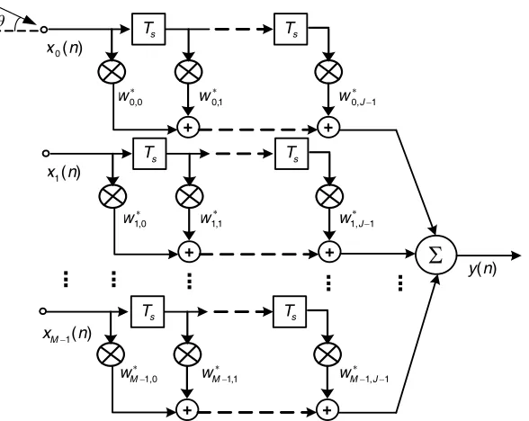
A wideband array processor based on uniform linear array is shown in Fig. 1, where J is the number of taps associated with each of the M sensor channels. Let the array sensors be uniformly spaced with the inter-element spacing d less than or equal to c/(2fh), where c is the wave propagation speed and fh is the maximum frequency of the desired signal. Its response with respect to frequency fi and look directionθ can be written as

H(fi, θ) =wHS(fi, θ) (1)

where fi ∈ B = [fl, fh] is the chosen discrete frequency in the frequency range of interest B, fl the minimum frequency, andwa M J×1 coefficient vector defined as

w= [w0,0, . . . , wM−1,0, . . . , wM−1,J−1]T (2)

theM J×1 steering vectorS(fi, θ) is given by

S(fi, θ) = [1, . . . , e−j2πfi(M−1)dsinθ/c, . . . , e−j2πfi(J−1)Ts, . . . , e−j2πfi((M−1)dsinθ/c+(J−1)Ts)]T (3)

whereTs is the sampling period.

The wideband LCMV problem [7] can be formulated as

min

w w

H_{Rw subject to C}H_{w=f (4)}

where Ris the autocorrelation matrix of the observed array data X,Ca constraint matrix, and f the response vector.

Let us assume that the desired signal steering vector is known exactly. Then the solution of the wideband beamformer is

w_opt= ˆR−_xx1C

CHRˆ−_xx1C

₋1

f (5)

where ˆR_xx is the sample correlation matrix given by

ˆ

R_xx= 1 L

L−1

n=0

X(n)XH(n) (6)

withL being the number of samples available and

3. PROPOSED ROBUST WIDEBAND BEAMFORMER

In practical situations, the signal steering vector may be known imprecisely, that is, the actual steering vector may differ from the presumed one. An essential shortcoming of the beamformer (7) is that it is not robust against such a steering vector mismatch and can severely suppress the desired signal. The actual steering vector of the desired signal from direction θ0 has been explicitly modeled as

ˆ

S(fi, θ0) =e(fi)+S(fi, θ0), e(fi) ≤ε (8) where S(fi, θs) is the assumed steering vector of the look direction θs, e(fi) an error vector, • the Euclidian norm, andεa small positive value.

Using the Cauchy-Schwarts inequality, it follows that

wHSˆ(fi, θ0)=wH(S(fi, θs) +e(f ))≥wHS(fi, θs)−wHe(fi) (9)

3.1. The Conventional Probability-Constrained Optimization Method

The existing probability-constrained optimization methods all assume that the steering vector errors are small enough to satisfy

wHS(fi, θs)>wHe(fi) (10) From the triangle inequality (9) it follows that

wH(S(fi, θs) +e(f))≥wHS(fi, θs)−wHe(fi) (11) Following [17–19], the probability-constrained robust wideband beamformer can be written as

⎧ ⎨ ⎩

min

w wHRˆxxw

s.t.Pr wHSˆ(fi, θ0)≥1

≥p fi∈[fl, fh]

(12)

wherep is a certain preselected probability value, and Pr{•} stands for the probability operator. Then the constraint in (12) can be approximated as

PrwHe(fi)≤wHS(fi, θs)−1

≥p fi∈[fl, fh] (13) Let e(fi) be drawn from a complex circularly symmetric Gaussian distribution with zero mean and covariance matrix C_e. Thus wH(S(fi, θs) +e(f)) has the complex Gaussian distribution with

wHS(fi, θs) mean and covariance matrix C

1/2

e w2. Since wH(e(f)) is circular zero mean complex Gaussian, its real and imaginary parts are real independent identically distributed Gaussian.

Using the Rayleigh-distributed, the Eq. (13) can be written as

PrwHe(fi)≤wHS(fi, θs)−1

= 1−exp ⎛ ⎜

⎝wHS(fi, θs)−1 2

C1_e/2w2

⎞ ⎟

⎠≥p (14)

Based on the distortion-less response constraint wHS(fi, θs)≥1, we can obtain

wH_Cew≤ 1

−ln(1−p)w H_S(f

i, θs)−1

(15)

Observing that the cost function in (12) is unchanged when wundergoes an arbitrary phase rotation, we can select wsuch that

RewHS(fi, θs)

≥0, ImwHS(fi, θs)

= 0 (16)

By Eqs. (15) and (16), the corresponding problem of the probability-constrained is formulated as follows ⎧

⎨ ⎩

min

w wHRˆxxw

s.t.wH_{Cew≤ √} 1 −ln(1−p)

wHS(fi, θs)−1

fi∈[fl, fh]

+ 0,0 w∗

0( )

x n

s

T Ts

+ 0,1

w∗ w0,J 1

∗ −

+

1( )

x n

s

T Ts

+

+

1( )

M

x ₋ n

s

T Ts

+ 1,0

M

w∗₋ wM 1,1

∗

− wM 1,J1

∗ − −

..

.

..

.

..

.

..

.

w∗ w1,1

∗

1,J1

w∗ −

Σ

..

.

θ

Figure 1. A general wideband beamforming structure.

3.2. Proposed RB-PC

Without the small steering vector errors assumption in (10), we propose a novel robust wideband beamformer based on probabilistic-constraint optimization which is called RB-PC.

Let us rewrite the constraint Pr wHSˆ(fi, θ0)≥1

≥p in (12) and (13) as

PrwHS(fi, θs)−wHe(fi)≥1

+ PrwHS(fi, θs)−wHe(fi)≤ −1

≥p (18) Using Eq. (14), we can obtain

PrwHS(fi, θs)−wHe(fi)≥1

= PrwHe(fi)≤wHS(fi, θs)−1

= 1−exp

−wHS(fi, θs)−1

2

wH_Cew

(19)

PrwHS(fi, θs)−wHe(fi)≤ −1

= 1−PrwHe(fi)<wHS(fi, θs)+ 1

= exp

−wHS(fi, θs)+ 1

2

wH_Cew

(20)

RewHS(fi, θs)

≥0, ImwHS(fi, θs)

= 0 (21)

Using (19)–(21), the problem of the proposed RB-PC can be approximated as

min

w wHRˆxxw

s.t. ImwHS(fi, θ0)

= 0

1−exp

−(wHS(fi,θ0)−1)2

wH_Cew

+ exp

−(wHS(fi,θ0)+1)2

wH_Cew

≥p fi ∈[fl, fh]

(22)

Let us define a variablet as

t=p−exp

−

wHS(fi, θs) + 1

2

wH_Cew

Then the cost function in (22) can be written as

exp

−

wHS(fi, θs)−1

2

wH_Cew

≤1−t (24)

Therefore, the problem of RB-PC can be written as

min

w wHRˆxxw

s.t. ImwHS(fi, θs)

= 0

wH_Cew≤ √ 1 −ln(1−t)

wHS(fi, θs)−1

fi ∈[fl, fh]

(25)

The RB-PC method imposes a group of constraints on the chosen discrete frequency to prevent the mismatched desired signal from being suppressed by the beamformer. However, the inconsistency of the frequency response of the wideband beamformer may cause severe distortion to the mismatched desired signal. Moreover, too many constraints can decrease the number of degrees of freedom. As a result, the performance of interference cancellation may drop significantly.

3.3. Proposed RB-FI-PC

To improve the performance of RB-PC method, an efficient method called response variation (RV) can be employed to control consistency of the frequency response over the frequency-angle range of interest [16]. The parameter RV is given by

RV = 1

NfNΘ

Nf

i=1

NΘ

j=1

[S(fi, θj)−S(fr, θj)][S(fi, θj)−S(fr, θj)]H (26)

where N• denotes the number of the sampling points, Θ the angle range over which RV is considered, andfrthe reference frequency. If RV is small enough, the beamformer has a better consistent frequency response over f and Θ.

The parameter RV can be transformed to

RV =wHCw (27)

where

C= 1

NBNΘ

NΘ

j=1

Nf

i=1

|S(fi, θj)−S(fr, θj)|2 (28)

We define a thresholdγ to constraint the parameter RV

RV =LH₁ w2 ≤γ (29)

where L1 = U1Λ11/2, with Λ1 being the eigenvalue matrix of C, and U1 being the corresponding eigenvector matrix. Similar to (29), we can get

wHRˆ_xxw=LH₂ w2 (30)

Then the robust wideband beamformer with the RV constraint (RB-FI-PC) can be approximated as

min

w L

H

2 w 2

s.t. ImwHS(fr, θs)

= 0

wH_Cew≤ √ 1 −ln(1−t)

wHS(fr, θ0)−1

θs

w2 < γw

LH₁ w2≤γ

(31)

3.4. Optimization Problem Solution Using Iterative SOCP

Since the solution processing of the RB-PC method is the same as the RB-FI-PC method, next we will give the solution of RB-FI-PC by using iterative SOCP method.

Note that

t=p−exp

−

wH_S(f

r, θs) + 1

2

wH_Cew

= 1−p−

1−exp

−

wH_S(f

r, θs) + 1

2

wH_Cew

< p (32)

For initialization of the iterative SOCP, we can choose t0 =p and obtain the initial weight vector w0 by the SOCP method.

Using the estimated weight vectorw_k−1 of (31) to update the variable tk in (23) as

tk=p−exp

−

wH_k−1S(fr, θs) + 1

2

wH_k−1C_ew_k−1

(33)

To guarantee the estimatedw_k−1always be in feasible regions, we should check the value of the function Φ(w_k−1) before the new iteration

Φ(w_k−1) = exp

−

wH_k−1S(fr, θs)−1

2

wH

k−1Cewk−1

−exp

−

wH_k−1S(fr, θs) + 1

2

wH

k−1Cewk−1

≤1−p (34)

Ifw_k−1 cannot satisfy the constraint in (34), we will employ the following measures. For any constantβ ≥1, we can get

(βw_k−1)HS(fr, θs)−1

2

(βw_k−1)HCe(βwk−1) ≥

(βw_k−1)HS(fr, θs)−β

2

(βw_k−1)HCe(βwk−1) =

wH_k−1S(fr, θs)−1

2

wH_k−1C_ew_k−1

(35)

(βw_k−1)HS(fr, θs) + 1

2

(βw_k−1)HCe(βwk−1) ≤

(βw_k−1)HS(fr, θs) +β

2

(βw_k−1)HCe(βwk−1) =

wH

k−1S(fr, θs) + 1 2

wH

k−1Cewk−1

(36)

It is easy to observe that the function Φ(βw_k−1) is a decreasing function on constantβ. As a result, there always exists a suitable β to make βw_k−1 satisfy the constraint in (34). The constant β can be directly obtained by some conventional one-dimension search schemes.

When the absolute value |tk−tk−1| drops below a certain pre-specified threshold, it is assumed that the variablethas adapted optimally and the iterative procedure can stop. Otherwise the iterative process should continue until it reaches convergence. Fortunately, it only needs 2 to 3 times of iterative to achieve convergence according to numbers of experiments.

For an iterative algorithm, we need present the convergence proof of the optimization algorithm based on iterative SOCP theory. First of all, let us prove that the sequence {tk} is a monotone non-increasing sequence in the iteration process. For a known tk, the Eq. (31) is a convex optimization problem. As a result, the optimum weightw_k can be obtained.

Using the KKT condition in (31), we can obtain tk as

tk= 1−exp

−

wH_kS(fr, θs)−1

2

wH kCewk

(37)

On the other hand, we know that

tk+1 =p−exp

−

wH_kS(fr, θs) + 1

2

wH kCewk

(38)

Therefore, we can get

tk+1−tk= exp

−

wH

kS(fr, θs)−1

2

wH_kC_ew_k

−exp − wH

kS(fr, θs) + 1

2

wH_kC_ew_k

Using Eq. (34), it is easy to find that tk+1−tk ≤0, so the sequence{tk} is a monotone non-increasing sequence in the iteration process. Therefore, we can verify that whenk→ ∞, there always exits a lower boundtopt>0 to make the sequence{tk}convergent. Furthermore, whenk→ ∞, the optimum weight

{w_k} can also converge to the optimum value w_opt.

So we can summarize the proposed algorithm as follows

Step 1. Selecting the initial value t0 =p, we can obtain the initial weight vector w0 by applying the SOCP method in (31).

Step 2. For k >1, if thek−1th weight vector w_k−1 is content with (34), the tk can be obtained by (33). If not, let us choose the appropriate constant β ≥1 through one-dimension search algorithm, and replacew_k−1 by βwk−1 to obtain the updatedtk. Then, the weight vector wk can be obtained by (31).

Step 3. If the absolute value|tk−tk−1|drops below a certain pre-specified threshold, the variablet and the weight vector w have adapted optimally and the iterative procedure can stop. Otherwise, the iterative process should return to step 2 to continue until it reaches convergence.

4. SIMULATIONS

In our simulation, we compare the proposed RB-FI-PC beamformer in (31) with the RB-PC beamformer in (25), the RB-WC beamformer and the RB-FI-WC beamformer in [15]. A total of 200 independent Monte-Carlo runs are used to obtain each point.

They are performed based on a ULA with M = 15 and J = 20, the frequency range of interest is between 800 MHz and 1300 MHz, the reference frequency is 1050 MHz, the number of the chosen discrete frequencies is 18. The covariance matrixC_e can be approximated asσ2I_{M K} [20], where σ2 is 0.4. Sample number is set to 512 in each simulation.

The actual desired signal comes from θ0 = 0◦ with a signal-to-noise ratio (SNR) of 10 dB. Two wideband interferences arrive from −30◦ and 45◦, respectively, with a signal-to-interference (SIR) of

−30 dB. In the following, the presumed look direction is θs = 4◦. For the RB -PC beamformer, p is set to be 0.95; for the RB-FI-PC beamformer, the value of γ = 0.0007 andp = 0.95 is chosen; for the RB-WC beamformer, ε is set to be 4.5; for the RB-FI-WC beamformer, ε = 3.1 and ς = 0.013 are chosen.

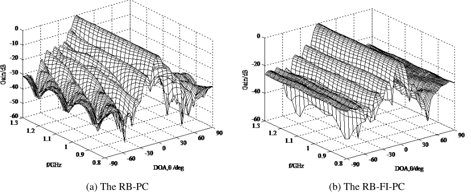
The resultant beam pattern of the RB-PC and the RB-FI-PC is shown in Fig. 2(a) and Fig. 2(b), respectively, which shows an effective robustness of the wideband beamformer against look direction

(a) The RB-PC (b) The RB-FI-PC

errors and forms two nulls at−30◦ and 45◦ to suppress two interfering signals. Furthermore, the RB-FI-PC beamformer has a better performance in terms of frequency invariant property over the RV angle range, response variation control and interference suppression.

Figure 3 shows the output SINR versus the probabilitypfor the wideband beamformers. Generally, the probabilitypcannot smaller than 0.9. To observe the change trend of output SINR with the varied p, we expand the range ofpto 0.1∼1. With the increasing value ofp, we can see that the output SINRs for both proposed beamformers improve gradually. When the probabilityp≥0.9, the output SINRs of proposed RB-FI-PC method will stay higher than 20 dB with little fluctuation.

Let us set constraint parameters as p= 0.95, σ2 ∈[0.1,1] and γ ∈[0.0001,0.001]. Fig. 4(a) shows the output SINR versus the parameterσ2 of the RB-PC method. Since the largerσ2 denotes the larger steering vector mismatch, the output SINR performance decreases drastically with the increasing σ2 in [0.4 ∼ 1]. However, when σ2 ∈[0.1 ∼0.4], the larger σ2 brings the better output SINR. Because too

0.1 0.91 0.94 0.97 1

-10 -5 0 5 10 15 20 25

p

out

p

ut

S

IN

R

/dB

RB-FI-PC RB-PC

Figure 3. Output SINR versus the probabilityp.

σ2

0.2 0.4 0.6 0.8 1

3 4 5 6 7 8 9 10 11 12 13 14

σ2

γ

-5 -5

-5 0

0

0

0 ₀

0

0

5

5

5

5 5

5

5

5 5

10

10

10

10

10 10 10

15

15

15

15

15

20

20

20

20

21

21

21

21

0.1 0.2 0.3 0.4 0.5 0.6 0.7 0.8 0.9 1

1 2 3 4 5 6 7 8 9

10x 10

-4

(a) The RB-PC (b) The RB-FI-PC

many constraints narrowed the scope of optimal solution set, the appropriate increase ofσ2 is equivalent to enlarge the set of optimal solutions, thus the output performance of SINR increased. Fig. 4(b) shows the output SINR versus the parameter σ2 _{of the RB-FI-PC method. Following the increase of σ}2_{, in} order to obtain the better SINR performance, the selection range of parameter γ is smaller. When the other conditions remain unchanged, the largerσ2can decrease the output SINR performance. Therefore, we should select those parameters reasonably to achieve the best output performance.

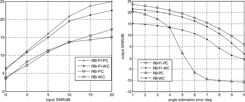
Figure 5 shows the output SINR versus the input SNR for the RB-FI-PC, the RB-FI-WC, the RB-PC, and the RB-WC beamformer. Obviously, the RB-FI-PC has obtained the highest output SINR than the other beamformers for the input SNRs in [−2 ∼ 20] dB. The worst-case mismatch of the RB-FI-WC and RB-WC beamformer may actually seldom occur in practical applications, so the over conservative constraint can degrade the output performance. However, when the input SNRs is lower than−2 dB, the output SINR of RB-FI-WC is slightly higher than the proposed RB-FI-PC due to the worse initialt of RB-FI-PC in the low SNR condition.

In the last, we study their performance in terms of output SINR versus look direction error, and the result is shown in Fig. 6. It can be seen that the RB-FI-PC beamformer has the best robustness than others against the look direction error. For large look direction errors, the performance of the RB-PC beamformer decreases significantly due to the extra consumption of degrees of freedom caused by the frequency response inconsistency.

-5 0 5 10 15 20

0 5 10 15 20 25

input SNR/dB

out

put

S

IN

R

/d

B

RB-FI-PC RB-FI-WC RB-PC RB-WC

Figure 5. Output SINR versus input SNR with an angle estimation error of 4◦.

1 2 3 4 5 6 7 8 9 10

-15 -10 -5 0 5 10 15 20 25

angle estimation error /deg

output SINR/dB

RB-FI-PC RB-FI-WC RB-PC RB-WC

Figure 6. Output SINR versus the look direction error.

5. CONCLUSION

A novel robust wideband beamformer with frequency invariance constraints is proposed based on the probability-constrained optimization. By employing the RV element, we can control the frequency invariant property of the adaptive wideband beamformer in the look direction region over the frequency range of interest. The optimum coefficient vector is obtained by a proposed iterative SOCP method without the small steering vector errors assumption. Simulation results have validated a superior performance of the proposed wideband beamformer as compared to robust wideband beamformer based on worst-case performance optimization.

REFERENCES

2. Yang, K., Z. Zhao, and Q. H. Liu, “Robust adaptive beamforming against array calibration errors,”

Progress In Electromagnetics Research, Vol. 140, 341–351, 2013.

3. Li, Y., Y. J. Gu, Z. G. Shi, and K. S. Chen, “Robust adaptive beamforming based on particle filter with noise unknown,”Progress In Electromagnetics Research, Vol. 90, 151–169, 2009.

4. Gu, Y. J., Z. G. Shi, K. S. Chen, and Y. Li, “Robust adaptive beamforming for a class of Gaussian steering vector mismatch,” Progress In Electromagnetics Research, Vol. 81, 315–328, 2008.

5. Vook, E. W. and R. T. Compton, Jr., “Bandwidth performance of linear adaptive arrays with tapped delay-line processing,” IEEE Trans. Aerosp. Electron. Syst., Vol. 28, No. 3, 901–908, Jul. 1992.

6. Lin, N., W. Liu, and R. J. Langley, “Performance analysis of an adaptive broadband beamformer based on a two-element linear arraywith sensor delay-line processing,” Signal Processing, Vol. 90, 269–281, Jan. 2010.

7. Frost, III, O. L., “An algorithm for linearly constrained adaptive array processing,” Proc. IEEE, Vol. 60, No. 8, 926–935, Aug. 1972.

8. Van Veen, B. D. and K. M. Buckley, “Beamforming: A versatile approach to spatial filtering,”

IEEE Acoust., Speech, Signal Processing Mag., Vol. 5, No. 2, 4–24, Apr. 1988.

9. Brandstein, M. S. and D. Ward, Microphone Arrays: Signal Processing Techniques and Applications, Springer, Berlin, Germany, 2001.

10. Li, J. and P. Stoica, Robust Adaptive Beamforming, Wiley, Hoboken, NJ, 2005.

11. Carlson, B. D., “Covariance matrix estimation errors and diagonal loading in adaptive arrays,”

IEEE Trans. Aerosp. Electron. Syst., Vol. 24, 397–401, Jul. 1988.

12. Er, M. H. and A. Cantoni, “Derivative constraints for broadband element space antenna array processors,” IEEE Trans. Antennas Propag., Vol. 31, No. 6, 1378–1393, Dec. 1983.

13. Rubsamen, M. and A. B. Gershman, “Robust presteered broadband beamforming based on worst-case performance optimization,” Proc. IEEE Workshop on Sensor Array and Multichannel Signal Processing, 340–344, Darmstadt, Germany, Jul. 2008.

14. El-Keyi, A., T. Kirubarajan, and A. B. Gershman, “Wideband robust beamforming based on worst-case performance optimization,” Proc. IEEE Workshop on Statistical Signal Processing, 265–270, Bordeaux, Jul. 2005.

15. Zhao, Y., W. Liu, and R. J. Langley, “Adaptive wideband beamforming with frequency invariance constraints,” IEEE Trans. Antennas Propag., Vol. 59, No. 4, 1175–1184, Apr. 2011.

16. Duan, H., B. P. Ng, C. M. See, and J. Fang, “Applications of the SRV constraint in broadband pattern synthesis,”Signal Processing, Vol. 88, 1035–1045, Apr. 2008.

17. Vorobyov, S. A., Y. Rong, and A. B. Gershman, “Robust adaptive beamforming using probability-constrained optimization,”Proc. IEEE Stat. Signal Process. Workshop, 934–939, Bordeaux, France, Jul. 2005.

18. Vorobyov, S. A., Y. Rong, and A. B. Gershman, “On the relationship between robust minimum variance beamformers with probabilistic and worst-case distortionless response constraints,” IEEE Transactions on Signal Processing, Vol. 56, No. 11, 5719–5725, Nov. 2008.

19. Wang, W., C. Liu, and Y. Zhao, “A novel probability-constrained approach to robust wideband beamforming with sensor delay lines,” IET International Radar Conference 2013, Xian, Shanxi, Apr. 2013.