Two-Degree-of-Freedom Control Scheme for Robust Centralized PI/PID Controller Design Using Constrained Optimization

Vol. 1, No. 1, pp. 1-8, June (2018)

Two-Degree-of-Freedom Control Scheme for Robust Centralized PI/PID

Controller Design Using Constrained Optimization

Amir Afroomanda)_{andSaeed Tavakoli}b)

For a two-input two-output distillation column with heavy interactions and long dead times, a two-by-two PI/PID controller is designed. The design objectives are good setpoint regulation and appropriate load disturbance rejection. The constraints are on degree of robust stability, control effort as well as peaks of the maximum singular value of sensitivity and complementary sensitivity matrices. As this set of design objectives and constraints is often conflicting, a more flexible control structure, a two-degree-of-freedom scheme, is proposed. The design problem is formulated as a constrained optimization problem and is solved by a powerful random-search optimization technique, the so-called vector-based swarm optimization. Next, the performance of the proposed method in controlling a Wood and Berry distillation column is evaluated and compared with that of several well-known design techniques. Because of using a flexible control structure, a powerful optimization algorithm and a comprehensive set of design requirements, the proposed control strategy performs well in coping with conflicting design objectives.

A B S T R A C T

ARTICLE INFO

Keywords:

Load Disturbance Rejection Robustness

Setpoint Regulation

Two-Degree-of-Freedom Control Structure Wood and Berry Distillation Column Article history:

Received February. 13, 2018 Accepted Aprill. 12, 2018

I. INTRODUCTION

Due to its noticeable effectiveness and simple struc-ture, PID is the most popular industrial controller and any improvement in the PID control tuning is valuable1_.

The PID has only three parameters, however, it is not easy to find its optimal values without a systematic procedure2. For single-input single-output (SISO) and multiple-input multiple-output (MIMO) systems, a huge number of analytical and numerical techniques for tun-ing PID controllers have been presented durtun-ing the past decades3–5_{. In general, the problem of PID control}

de-sign for MIMO plants can be categorized to 1) multi-loop PID controller design, 2) decentralized PID controller de-sign using a de-coupler, and 3) centralized PID controller design.

a)_{Department of Electrical and Computer Engineering, University} of Sistan and Baluchestan, Zahedan, Iran

b)_{Corresponding Author: [email protected], Tel:} +98-54-31136556, Fax: +98-54-33447186, Department of Electrical and Computer Engineering, University of Sistan and Baluchestan, Za-hedan, Iran

http://dx.doi.org/10.22111/ieco.2018.24006.1007

In this research work, the case study is a input two-output (TITO) industrial plant, the Wood and Berry dis-tillation column6. Due to strong interactions between its inputs and outputs as well as long dead times, it is a chal-lenging benchmark application. The distillation column should be controlled in such a way that the design specifi-cations are satisfied and the resulting closed-loop system is robust in the face of model uncertainties. Several pa-pers have been published on setpoint regulation and/or load disturbance rejection of this TITO plant. Using a decentralized PI controller, Tavakoli et al.7_{proposed a}

ro-bust non-dimensional tuning technique to simultaneously obtain good responses to setpoint and load disturbance signals. Based on the direct synthesis method, a central-ized PI controller using relative gain array (RGA) and relative normalized gain array (RNGA) was presented8_.

Also, a centralized PI controller based on steady-state gain matrix (SSGM) was designed9.

In this paper, the design goal is to obtain good re-sponses for both setpoint and load disturbance signals. Also, a number of constraints on degree of robust sta-bility, control effort, and peaks of the maximum singular value of sensitivity and complementary sensitivity matri-ces are considered. This set of objectives and constraints is often conflicting. In fact, it is a difficult task to find a good trade-off solution using a one-degree-of-freedom (1DoF) control scheme. To obtain better trade-off so-lutions, a two-degree-of-freedom (2DoF) control scheme is employed. First, the PID control design problem is formulated as an optimization problem. As the resulting problem is challenging, a powerful optimization tool is re-quired to find its optimal solution. To achieve this goal, an easy to use, reliable and robust optimization algo-rithm, named vector-based swarm optimization (VBSO) is used10,11_.

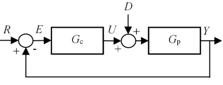
FIG. 1. Block diagram of a 1DoF control system.

FIG. 2. Block diagram of a 2DoF control scheme.

and the optimal PID parameters are obtained using VBSO. Also, the proposed controllers are compared with other design methods and concluding remarks are pro-vided. Finally, the conclusions of the study are drawn in SectionV.

II. CONTROL STRUCTURE AND DESIGN

REQUIREMENTS

Block diagram of a 1DoF closed-loop control system is shown in Fig. 1. Gp and Gc refer to n×n plant and

controller matrices, respectively. R, Y and D are refer-ence input, output and load disturbance vectors, respec-tively. Also,EandU represent error and control vectors. To design a centralized PID controller with a filter on the derivative action, the elements ofGc are defined as gcij =kcij +kiij/s+ (kdijs)/(1 + 0.1kdij/kcijs)i, j ∈ {1, ..., n}, where kcij, kiij, kdij are the proportional,

in-tegral and derivative gains fromjth _{input toi}th_output,

respectively.

Block diagram of the proposed 2DoF closed-loop control system is shown in Fig. 2, where

Gff = diag(gff 1, gff 2, . . . , gff n), bi is the setpoint

weight,gffi= (bikcii+kiii/s+kdiis/(1 + 0.1kdii/kciis)),

Gc1 =

g0_cij n×n, g

0

cij = gcij/gcjj and Gc2 =

diag (gc11, gc22, . . . , gcnn) .

It is worth noting that the setpoint weight has a signif-icant influence on the response to setpoint signals. How-ever, it has no influence on disturbance response or robust stably criteria.

According to Fig. 2, the output of closed-loop sys-tem is Y = (I + GpGc1Gc2)−1GpGc1GffR + (I + GpGc1Gc2)−1GpD. Also, sensitivity and

comple-mentary sensitivity matrices are respectively S = (I + GpGc1Gc2)−1 = (I + L)−1 and T =(I + GpGc1Gc2)−1GpGc1Gff, where L = GpGc1Gc2 is the

loop transfer matrix. Note that Gff = Gc2 for bi = 1.

In addition,Gff ≈Gc2 for low and high frequencies. To

reach acceptable setpoint regulation over low frequencies,

T should be approximately an identity matrix. There-fore,S should be very small as T+S ≈ I. Hence, the maximum singular value ofS, ¯σ(I+L)−1, should be small or the minimum singular value ofL, σ[L], should be large. Considering the second term ofY, however, it may not lead to a good disturbance rejection. To reduce sensitivity to modelling errors, the resulting closed-loop system should not be too sensitive to variations in the plant dynamics. To achieve this goal, the maximum sin-gular value of S should be small. The transfer matrix from R to U, a measure of control effort, is defined by

Q= (I+Gc1Gc2Gp)−1Gc1Gff.

Here, a well-known method for checking robust sta-bility is used12,13_{. Considering output multiplicative}

uncertainty, the 2DoF closed-loop system will remain stable under the uncertainty ∆o if and only if l(ω) <

1

¯

σ

(I+L)−1_L

=σ

I+ (L)−1

. As the plant can be modelled more accurately in small frequencies, l(ω) in ¯

σ[∆(jω)] ≤ l(ω) ≤ γ is small at low frequencies. In fact,γindicates the degree of robust stability. Similarly, for input multiplicative uncertainties, the closed-loop sys-tem will remain stable under the uncertainty ∆i if and

only ifl(ω)<1σ¯(I+LI)−1LI

=σI+L−_I1 , LI = Gc1Gc2Gp.

In Fig. 2, the aim of design is to determine the pa-rameters ofGc1,Gc2 and Gff so that the outputs follow

the reference signals in spite of load disturbances, mea-surement errors and model uncertainties. In fact, the IAE criteria for unit step changes in setpoint and load disturbance inputs should be minimized.

To obtain a robust controller with good performance, four constraints on kSk_∞, kTk_∞, kQk_∞ and γ should be considered. In fact, a high degree of robustness is achieved by having large enough values ofγand by avoid-ing large peaks in ¯σ(S).

The design procedure has two main phases. In the first phase, setpoint signals are zero andGc1 andGc2are

determined so that step load disturbance signals are ap-propriately rejected whereas above-noted constraints are satisfied. In the second phase, load disturbance signals are zero and setpoint weights are tuned to achieve good setpoint responses.

III. VBSO ALGORITHM

Evolutionary and nature-inspired algorithms are in-creasingly used in numerical optimization problems. These algorithms are less likely to get trapped in local extrema in comparison with single-solution based meth-ods or gradient based methmeth-ods. To solve a variety of opti-mization problems, evolutionary and nature-inspired op-timization algorithms, such as genetic algorithm (GA)14_,

years. Also, their advantages and disadvantages have been identified and several improved strategies have been provided19–25_.

In this paper, a vector-based swarm optimization (VBSO) algorithm with high accuracy and high speed of convergence, proposed by Afroomand & Tavakoli, is used10,11. It is an easy to understand, easy to use, reli-able and robust optimization algorithm, which performs on the vectors in a D-dimensional search space. Each vector represents a solution. Vectors with appropriate orientation gradually converge to global optimum point. The main idea in VBSO is to use the cooperation oper-ator. It is divided in direct cooperation vector, orienting solutions towards the global optimum point, and differen-tial cooperation vector, responsible for small-scale search around the direct cooperation vector. Differential coop-eration vector helps the algorithm to pass local optimums and converge to global one. The direct and differential cooperation vectors are formed using multiplication of VBSO weighting coefficients by suitable vectors. The pseudo code of VBSO algorithm is as follows.

First, an initial population havingNpop number of D

dimensional vectors is produced randomly. In the ini-tial population, Vi,j[0] is the value of jth element ofith

vector, where i ∈ [1, Npop] and j ∈ [1, D]. Also, vlowj

and vup_j are lower and upper limits of jth _{element of}

corresponding vector, respectively, and rand denotes a uniformly distributed random value in the interval (0,1). Second, each vector is evaluated according to a given cost function. Inkth_{iteration, the cooperation operator,} VCo[k], is determined using the direct and differential

cooperation vectors, VDir−C[k] and VDif−C[k]. These

cooperation vectors are formed using multiplication of VBSO weighting coefficients,w1−w9, byVc,Va,Vb, Vlb

andVr vectors. The first three vectors represent current

solution, average of solutions and current best solution, respectively. Also,Vlbis the best vector in the

neighbor-hood ofithvector andVr is a random vector. Figures 3

and4 show the contour lines of cost functions in a two-dimensional search space. Fig. 3 shows that suitable

VDir−C can be formed by considering proper portions of Vb and Vlb. Also, Fig. 4 illustrates howVDif−C is made

usingVc, Vb andVlb.

To increase the population diversity, a mutation oper-ator is used. Due to using cooperation vectors, VBSO al-gorithm has an intrinsic mutation capability. Moreover, a polynomial mutation is employed with a mutation prob-ability of 0.4, in which one or two elements of a selected vector are mutated. To make sure new vectors are inside the search space, a boundary check is also required at each step. In addition, the next population is selected from parents and offsprings based on fitness numbers. In

Vector-based swarm optimization algorithm

Set: D, Npop, Number of Iterations (NI),vlowj ,v up

j , Iteration=0 Vi,j[0] =vjlow+rand. v

up j −vjlow

,∀i= 1,2, ..., Npop, and j= 1,2, ..., D

While(Iteration≤NI)do

for i= 1,2, ..., Npop do

Calculate f(Vi)∀i= 1,2, ..., Npop, and V = (Vi1, V

2

i , ..., V D i )

Determine (Vb,Vlb,Vr,Va)

Generate weighting coefficients (w1−w9)

Direct CooperationVDir−C[k] =w1Vc[k] +w2Va[k] +w3Vb[k] +w4Vlb[k] +w5Vr[k]

Differential Cooperation VDif−C[k] =w6.(Va[k] −Vc[k]) +w7.(Vb[k]−Vc[k])

+w8.(Vlb[k]−Vc[k]) +w9.(Vr[k]−Vc[k])

VCo[k] =VDir−C[k] +VDif−C[k]

Mutation, Boundary Check, Next Generation Selection

end for

Iteration=Iteration+1

2 i D

Contour lines of cost functions

Global Optimum

1 i D b

V lb V

Dir C

V _

FIG. 3. Formation of the direct cooperation vector10_.

Contour lines of cost functions

Global Optimum

2 i D

1 i

D

b V

D if C

V 

lb V

c V

FIG. 4. Formation of the differential cooperation vector10_.

a minimization problem, the parents and offsprings are evaluated and sorted in an ascending order and the first

Npop vectors are transferred into the next population.

In the VBSO, there are several weighting coefficient se-lection strategies10,11. In this research work, the weight-ing coefficients are given bywi = 0.5 rand, i= 1,3,4,5, wi= 0.33rand, i= 7,8,9 andwi= 0rand, i= 2,6.

IV. SIMULATION

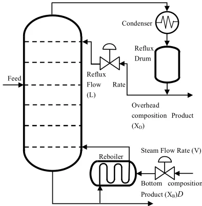
Most industrial plants are multi-input multi-output systems, in general. As a challenging industrial plant, a distillation column is studied in this section. A dis-tillation column is a process in which a liquid or vapor

Bottom composition

Product (XB)D Steam Flow Rate (V) Reboiler

Reflux Drum Condenser

Feed Reflux

Flow Rate (L)

Overhead composition Product (XD)

FIG. 5. Simple schematic of a distillation column.

mixture of two or more substances is separated into its component fractions of desired purity. Having strong in-teractions between its inputs and outputs, it is the most common separation technique. Fig. 5 depicts a simple distillation column.

The dynamic model of the Wood and Berry (WB) dis-tillation column, is given by

XD XB

=



 

12.8e−s

1 + 16.7s

−18.9e−3s

1 + 21s

6.6e−7s

1 + 10.9s

−19.4e−3s

1 + 14.4s



 

L V

(1)

whereXDandXB represent the percentage of methanol

in the distillate and bottom products, respectively. L

andV are the reflux and steam flow rates in the reflux drum and reboiler, respectively6,26.

Applying unit step functions to the reference inputs and step functions of 0.25 to the disturbance inputs, the objective function used isIAE=IAE1+IAE2, IAEi = R∞

0 |ei(t)|dtwhere IAEi and ei(t) denoteIAE criteria

The values of the performance and robustness indices are given by TableI.

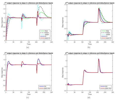
The output responses to steps in reference and load disturbance inputs are depicted in Fig. 6.

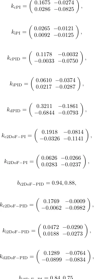
The PI and PID controller parameters are as follows.

kcPI=

0.1675 −0.0274 0.0286 −0.0825

,

kiPI=

0.0265 −0.0121 0.0092 −0.0125

,

kcPID=

0.1178 −0.0032

−0.0033 −0.0750

,

kiPID=

0.0610 −0.0374 0.0217 −0.0287

,

kdPID=

0.3211 −0.1861

−0.6844 −0.0793

,

kc2DoF−PI =

0.1918 −0.0814

−0.0326 −0.1141

,

ki2DoF−PI=

0.0626 −0.0266 0.0283 −0.0237

,

bi2DoF−PID= 0.94,0.88,

kc2DoF−PID=

0.1769 −0.0009

−0.0062 −0.0982

,

ki2DoF−PID=

0.0472 −0.0290 0.0188 −0.0273

,

kd2DoF−PID=

0.1289 −0.0764

−0.0899 −0.0834

,

bi2DoF−PI= 0.84,0.75.

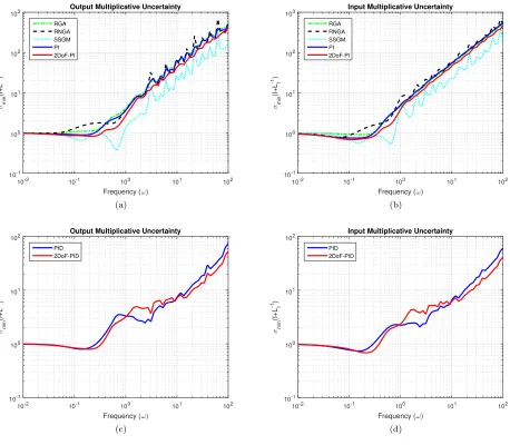
The stability regions of output and input uncertainties for closed-loop systems are depicted in Fig. 7. In this figure, the region above each curve represents the insta-bility region whereas the region below each curve repre-sents the stability region.

The plots of ¯σ(S) and ¯σ(T) for closed-loop systems are given by Fig. 8. They usually have peaks larger than one around the crossover frequencies. For real systems, these peaks are undesirable but unavoidable13_.

A good controller should provide a good compromise between performance and robustness. The controller pro-posed by SSGM method neither does give a satisfactory degree of robustness nor a good performance index ac-cording to Table I and Figures6and7. TableIand Fig.

7show that RGA and RNGA lead to large enough values ofγout. In addition, the peaks of ¯σ(S) in Fig. 8are small

enough for these two methods and, therefore, a high de-gree of robustness is anticipated. According to Table I

and Fig. 6, however, they result in big IAE criteria and, hence, unsatisfactory time responses. Moreover, the val-ues of ¯σ(S) are not small enough in low frequencies and, hence, inferior responses to load disturbance inputs are expected.

According to TableI and Figures6-8, the results pro-vided by proposed PI controllers are satisfactory in terms of the performance and robustness indices. As expected, the best result is provided by the proposed 2DoF-PI. For PID controllers, Table I along with Figures 6-8 reveal that the results provided by proposed PID controllers are satisfactory. Again, the best result is provided by the proposed 2DoF-PID.

Table I shows that the proposed 2DoF controllers per-form better than those in a 1DoF scheme considering both the performance and robustness indices. This is due to using the setpoint weighting. However, it leads to increasing the control effort. In addition, this table shows that the 2DoF-PID controller performs better than the 2DoF-PI controller. However, using an extra controller parameter, namely the derivative action, results in in-creasing the control effort.

Overall, simulation and comparison results confirm that the proposed method is better than other methods in terms of the performance and robustness. This is due to using a more flexible control structure, a more pow-erful optimization algorithm and a more comprehensive set of design requirements.

V. CONCLUSIONS

Time

0 50 100 150 200 250 300

Step response

0 0.2 0.4 0.6 0.8 1 1.2 1.4 1.61

st _{output response to steps in reference and disturbance inputs}

RGA RNGA SSGM PI 2DoF-PI

(a)

Time

0 50 100 150 200 250 300

Step response

-0.5 0 0.5 1 1.5 2 2.52

nd _{output response to steps in reference and disturbance inputs}

RGA RNGA SSGM PI 2DoF-PI

(b)

Time

0 50 100 150 200 250 300

Step response

0 0.2 0.4 0.6 0.8 1 1.2 1.41

st _{output response to steps in reference and disturbance inputs}

PID 2DoF-PID

(c)

Time

0 50 100 150 200 250 300

Step response

-0.5 0 0.5 1 1.5 2 2.52

nd _{output response to steps in reference and disturbance inputs}

PID 2DoF-PID

(d)

FIG. 6. Output responses to steps in reference inputs and disturbances.

TABLE I. Performance and robustness indices

Performance index Robust stability Control effort

Method

IAE ||T||∞ γout γin ||S||∞ ||Q||∞

RGA 69.5 1.02 0.98 0.91 1.58 0.26

RNGA 83.0 1.00 1.00 0.78 1.49 0.24

SSGM 48.8 2.74 0.37 0.51 3.40 1.31

PI 44.5 1.12 0.89 0.75 1.69 0.28

2D-PI 32.9 1.12 0.83 0.68 1.79 0.36

PID 32.6 1.25 0.80 0.74 1.63 1.35

2D-PID 28.9 1.21 0.80 0.68 1.77 1.95

REFERENCES

1_{K. J. ˚Astr¨om, and T. H¨agglund,Advanced PID control, ISA-The}

Instrumentation, Systems and Automation Society, Chapter 6, 2006.

2_{S. Skogestad, “Simple analytic rules for model reduction and PID}

controller tuning,”Journal of process control, Vol. 13, No. 4, pp. 291-309, June 2003.

3_{D. E. Seborg, D. A. Mellichamp, T. F. Edgar, and F. J. Doyle,}

Process Dynamics and Control, John Wiley & Sons, 2010.

4_{G. K. McMillan, Tuning and Control Loop Performance,}

Mo-mentum Press, 2014.

5_{Q. G. Wang, Z. Ye, W. J. Cai, and C. C. Hang, PID Control for}

Multivariable Processes,Springer Berlin Heidelberg, 2008.

6_{W. L. Luyben, “Simple method for tuning SISO controllers in}

Pro-Frequency (ω)

10-2 10-1 100 101 102

σmin

(I+L

-1)

10-1 100 101 102 103

Output Multiplicative Uncertainty

RGA RNGA SSGM PI 2DoF-PI

(a)

Frequency (ω)

10-2 10-1 100 101 102

σmin

(I+L

I

-1)

10-1 100 101 102 103

Input Multiplicative Uncertainty

RGA RNGA SSGM PI 2DoF-PI

(b)

Frequency (ω₎

10-2 10-1 100 101 102

σmin

(I+L

-1)

10-1 100 101 102

Output Multiplicative Uncertainty

PID 2DoF-PID

(c)

Frequency (ω₎

10-2 10-1 100 101 102

σmin

(I+L

I

-1)

10-1 100 101 102

Input Multiplicative Uncertainty

PID 2DoF-PID

(d)

FIG. 7. Stability regions of output and input uncertainties.

Frequency (ω)

10-2 10-1 100 101 102

σmax

(S) &

σmax

(T)

10-4 10-3 10-2 10-1 100 101

RGA RNGA SSGM PI 2DoF-PI

(a)

Frequency (ω)

10-2 10-1 100 101 102

σmax

(S) &

σmax

(T)

10-2 10-1 100 101

PID 2DoF-PID

(b)

cess Design and Development, Vol. 25, No. 3, pp. 654-660, Jul. 1986.

7_{S. Tavakoli, I. Griffin, P. J. Fleming, “Tuning of decentralised}

PI (PID) controllers for TITO processes,”Control Engineering Practice, Vol. 14, No. 9, pp. 1069-1080, Sep. 2006.

8_{V. V. Kumar, V. S. R. Rao, and M. Chidambaram, “Centralized}

PI controllers for interacting multivariable processes by synthesis method,”ISA Transactions, Vol. 51, No. 3, pp. 400-409, May 2012.

9_{V. D. Ram, and M. Chidambaram, “Simple method of}

design-ing centralized PI controllers for multivariable systems based on SSGM,”ISA transactions, Vol. 56, No. 1, pp. 252-260, May 2015.

10_{A. Afroomand, and S. Tavakoli, “Vector-Based Swarm}

Optimiza-tion Algorithm,”Applied Soft Computing, Vol. 37, No. 1, pp. 911-922, Dec. 2015.

11_{A. Afroomand, S. Tavakoli, M. Tavakoli, “An Efficient}

Meta-heuristic Optimization Approach to the Problem of PID Tuning for Automatic Voltage Regulator Systems,”2016 IEEE Interna-tional Conference on Advanced Intelligent Mechatronics (AIM), pp. 1682-1687, 2016.

12_{W. S. Levine,The Control Handbook, Second Edition: Control}

System Fundamentals, 2nd ed., CRC Press, Chapter 9, 2017.

13_{S. Skogestad, and I. Postlethwaite,Multivariable Feedback}

Con-trol: Analysis and Design, Wiley, Chapter 2, 2005.

14_{D. E. Goldberg, Genetic Algorithms in Search, Optimization and}

Machine Learning,Addison-Wesley Longman, 1989.

15_{R. Eberhart, and J. Kennedy, “A new optimizer using particle}

swarm theory,”Micro Machine and Human Science, 1995 MHS ’95, Proceedings of the Sixth International Symposium on, pp. 39-43, 1995.

16_{R. Storn, and K. Price, “Differential Evolution - A Simple}

and Efficient Heuristic for Global Optimization over Continu-ous Spaces,”Journal of Global Optimization, Vol. 11, No. 4, pp. 341-359, Dec. 1997.

17_{Z. W. Geem, J. H. Kim, and G. Loganathan, “A new heuristic}

optimization algorithm: harmony search,”Simulation, Vol. 76, No. 2, pp. 60-68, Feb. 2001.

18_{Y. Xin-She, and S. Deb, “Cuckoo Search via Levy flights,”Nature}

& Biologically Inspired Computing, 2009 NaBIC 2009 World Congress on, pp. 210-214, 2009.

19_{A. Afroomand, A. Gharaveisi, and F. M. Pour, “A New}

Heuris-tic Algorithm for Optimizing PID Controller On AVR Sys-tems,”International Power System (PSC), 2011 26th Conference on, pp. 1-10, 2011.

20_{M. Mohseni, A. Afroomand, and F. Mohsenipour, “Optimum}

coordination of overcurrent relays using SADE algorithm,”16th Electrical Power Distribution Conference, pp. 1-10, 2011.

21_{F. M. Pour, A. Gharaveisi, A. Afroomand, and S. Mohammadi,}

“Optimizing a fuzzy logic controller for a photovoltaic grid inde-pendent system,”1st Annual Clean Energy Conference on Inter-national Center for Science, High Technology&Environmental Sciences, pp. 237-241, 2010.

22_{E. Valian, E. Mohanna, and S. Tavakoli, “Improved cuckoo}

search algorithm for global optimization,”International Journal of Communications and Information Technology, Vol. 1, No. 1, pp. 31-44, Dec. 2011.

23_{E. Valian, S. Mohanna, and S. Tavakoli, “Improved cuckoo search}

algorithm for feedforward neural network training,”International Journal of Artificial Intelligence &Applications, Vol. 2, No. 3, pp. 36-43, Jul. 2011.

24_{E. Valian, S. Tavakoli, S. Mohanna, and A. Haghi, “Improved}

cuckoo search for reliability optimization problems,”Computers &Industrial Engineering, Vol. 64, No. 1, pp. 459-468, Jan. 2013.

25_{E. Valian, S. Tavakoli, and S. Mohanna, “An intelligent global}

harmony search approach to continuous optimization

prob-lems,”Applied Mathematics and Computation, Vol. 232, No. 1, pp. 670-684, April 2014.

26_{R. Rajabioun, “Cuckoo optimization algorithm,”Applied soft}

computing, Vol. 11, No. 8, pp. 5508-5518, Dec. 2011.

Amir Afroomand was

born in Bandar Abbas, Iran, in 1985. He received his BSc and MSc degrees in Electrical Engineering from Shahid Bahonar University of Kerman, Iran, in 2009 and 2011, respectively. He is currently a PhD candidate in electrical engineering at the University of Sistan and Baluchestan, Iran. His current research interests include PID control, robust control, evolutionary algorithms, and multi-objective optimization.