Unified Expectation Maximization

Unified Expectation Maximization

Rajhans Samdani University of Illinois [email protected]

Ming-Wei Chang Microsoft Research [email protected]

Dan Roth University of Illinois

[email protected]

Abstract

We present a general framework containing a graded spectrum of Expectation Maximization (EM) algorithms called Unified Expectation Maximization (UEM.) UEM is parameterized by a single parameter and covers existing al-gorithms like standard EM and hard EM, con-strained versions of EM such as Constraint-Driven Learning (Chang et al., 2007) and Pos-terior Regularization (Ganchev et al., 2010), along with a range of new EM algorithms. For the constrained inference step in UEM we present an efficient dual projected gradient as-cent algorithm which generalizes several dual decomposition and Lagrange relaxation algo-rithms popularized recently in the NLP litera-ture (Ganchev et al., 2008; Koo et al., 2010; Rush and Collins, 2011). UEM is as efficient and easy to implement as standard EM. Fur-thermore, experiments on POS tagging, infor-mation extraction, and word-alignment show that often the best performing algorithm in the UEM family is a new algorithm that wasn’t available earlier, exhibiting the benefits of the UEM framework.

1 Introduction

Expectation Maximization (EM) (Dempster et al., 1977) is inarguably the most widely used algo-rithm for unsupervised and semi-supervised learn-ing. Many successful applications of unsupervised and semi-supervised learning in NLP use EM in-cluding text classification (McCallum et al., 1998; Nigam et al., 2000), machine translation (Brown et al., 1993), and parsing (Klein and Manning, 2004). Recently, EM algorithms which incorporate con-straints on structured output spaces have been pro-posed (Chang et al., 2007; Ganchev et al., 2010).

Several variations of EM (e.g. hard EM) exist in the literature and choosing a suitable variation is

of-ten very task-specific. Some works have shown that for certain tasks, hard EM is more suitable than reg-ular EM (Spitkovsky et al., 2010). The same issue continues in the presence of constraints where Poste-rior Regularization (PR) (Ganchev et al., 2010) cor-responds to EM while Constraint-Driven Learning (CoDL)1 (Chang et al., 2007) corresponds to hard EM. The problem of choosing between EM and hard EM (or between PR and CoDL) remains elusive, along with the possibility of simple and better alter-natives, to practitioners. Unfortunately, little study has been done to understand the relationships be-tween these variations in the NLP community.

In this paper, we approach various EM-based techniques from a novel perspective. We believe that “EM or Hard-EM?” and “PR or CoDL?” are not the right questions to ask. Instead, we present a unified framework for EM, Unified EM (UEM), that covers many EM variations including the constrained cases along with a continuum of new ones. UEM allows us to compare and investigate the properties of EM in a systematic way and helps find better alternatives.

The contributions of this paper are as follows:

1. We propose a general framework called Uni-fied Expectation Maximization (UEM) that presents a continuous spectrum of EM algo-rithms parameterized by a simple temperature-like tuning parameter. The framework covers both constrained and unconstrained EM algo-rithms. UEM thus connects EM, hard EM, PR, and CoDL so that the relation between differ-ent algorithms can be better understood. It also enables us to find new EM algorithms.

2. To solve UEM (with constraints), we propose

1

To be more precise, (Chang et al., 2007) mentioned using hard constraints as well as soft constraints in EM. In this paper, we refer to CoDL only as the EM framework with hard con-straints.

a dual projected subgradient ascent algorithm that generalizes several dual decomposition and Lagrange relaxation algorithms (Bertsekas, 1999) introduced recently in NLP (Ganchev et al., 2008; Rush and Collins, 2011).

3. We provide a way to implement a family of EM algorithms and choose the appropriate one, given the data and problem setting, rather than a single EM variation. We conduct experi-ments on unsupervised POS tagging, unsuper-vised word-alignment, and semi-superunsuper-vised in-formation extraction and show that choosing the right UEM variation outperforms existing EM algorithms by a significant margin.

2 Preliminaries

Letxdenote an input or observed features andhbe a discrete output variable to be predicted from a fi-nite set of possible outputsH(x). Let Pθ(x,h) be a probability distribution over(x,h) parameterized byθ. LetPθ(h|x)refer to the conditional probabil-ity ofhgivenx. For instance, in part-of-speech tag-ging,xis a sentence,hthe corresponding POS tags, andθcould be an HMM model; in word-alignment,

x can be an English-French sentence pair, h the word alignment between the sentences, and θ the probabilistic alignment model. Let δ(h = h0) be the Kronecker-Delta distribution centered ath0, i.e., it puts a probability of 1 ath0and 0 elsewhere.

In the rest of this section, we review EM and constraints-based learning with EM.

2.1 EM Algorithm

To obtain the parameterθ in an unsupervised way, one maximizes log-likelihood of the observed data:

L(θ) = logPθ(x) = log X

h∈H(x)

Pθ(x,h) . (1)

EM (Dempster et al., 1977) is the most common technique for learning θ, which maximizes a tight lower bound onL(θ). While there are a few different styles of expressing EM, following the style of (Neal and Hinton, 1998), we define

F(θ, q) =L(θ)−KL(q, Pθ(h|x)), (2)

where q is a posterior distribution over H(x) and

KL(p1, p2)is the KL divergence between two

dis-tributionsp1andp2. Given this formulation, EM can

be shown to maximizeFvia block coordinate ascent alternating overq(E-step) andθ(M-step) (Neal and Hinton, 1998). In particular, the E-step for EM can be written as

q = arg min q0_∈Q KL(q

0

, Pθ(h|x)) , (3)

whereQis the space of all distributions. While EM produces a distribution in the E-step, hard EM is thought of as producing a single output given by

h∗ = arg max

h∈H(x)

Pθ(h|x) . (4)

However, one can also think of hard EM as pro-ducing a distribution given byq = δ(h = h∗). In this paper, we pursue this distributional view of both EM and hard EM and show its benefits.

EM for Discriminative Models EM-like algo-rithms can also be used in discriminative set-tings (Bellare et al., 2009; Ganchev et al., 2010) specifically for semi-supervised learning (SSL.) Given some labeled and unlabeled data, such algo-rithms maximize a modifiedF(θ, q)function:

F(θ, q) =Lc(θ)−c1kθk2−c2KL(q, Pθ(h|x)) , (5)

where,q, as before, is a probability distribution over

H(x),Lc(θ)is the conditional log-likelihood of the labels given the features for the labeled data, andc1

andc2 are constants specified by the user; the KL

divergence is measured only over the unlabeled data. The EM algorithm in this case has the same E-step as unsupervised EM, but the M-step is different. The M-step is similar to supervised learning as it findsθ

by maximizing a regularized conditional likelihood of the data w.r.t. the labels — true labels are used for labeled data and “soft” pseudo labels based onqare used for unlabeled data.

2.2 Constraints in EM

con-text of EM, constraints can be imposed on the pos-terior probabilities, q, to guide the learning proce-dure (Chang et al., 2007; Ganchev et al., 2010).

In this paper, we focus on linear constraints over

h(potentially non-linear overx.) This is a very gen-eral formulation as it is known that all Boolean straints can be transformed into sets of linear con-straints over binary variables (Roth and Yih, 2007). Assume that we have m linear constraints on out-puts where thekthconstraint can be written as

ukTh≤bk .

Defining a matrix U asUT = u1T . . . umT

and a vectorbasbT = [b1, . . . , bm], we write down the set of allfeasible2structures as

{h|h∈ H(x),Uh≤b} .

Constraint-Driven Learning (CoDL) (Chang et al., 2007) augments the E-step of hard EM (4) by imposing these constraints on the outputs.

Constraints on structures can be relaxed to expec-tation constraintsby requiring the distributionq to satisfy them only in expectation. Define expecta-tion w.r.t. a distribuexpecta-tionq overH(x)asEq[Uh] = P

h∈H(x)q(h)Uh. In the expectation constraints

setting,qis required to satisfy:

Eq[Uh]≤b .

The space of distributionsQcan be modified as:

Q={q |q(h)≥0, Eq[Uh]≤b, X

h∈H(x)

q(h) = 1}.

Augmenting these constraints into the E-step of EM (3), gives the Posterior Regularization (PR) framework (Ganchev et al., 2010). In this paper, we adopt the expectation constraint setting. Later, we show that UEM naturally includes and generalizes both PR and CoDL.

3 Unified Expectation Maximization

We now present the Unified Expectation Maximiza-tion (UEM) framework which captures a continuum of (constrained and unconstrained) EM algorithms

2

Note that this set is a finite set of discrete variables not to be confused with a polytope. Polytopes are also specified as {z|Az≤d}but are over real variables whereashis discrete.

Algorithm 1The UEM algorithm for both the genera-tive (G) and discriminagenera-tive (D) cases.

Initializeθ0 fort= 0, . . . , T do

UEM E-step:

qt+1_{←arg min}

q∈QKL(q, Pθt(h|x);γ)

UEM M-step:

G:θt+1_{= arg max}

θEqt+1[logPθ(x,h)]

D:θt+1_{= arg max}

θEqt+1[logPθ(h|x)]−c1kθk2 end for

including EM and hard EM by modulating the en-tropy of the posterior. A key observation underlying the development of UEM is that hard EM (or CoDL) finds a distribution with zero entropy while EM (or PR) finds a distribution with the same entropy asPθ (or close to it). Specifically, we modify the objective of the E-step of EM (3) as

q= arg min q0_∈Q

KL(q0, Pθ(h|x);γ) , (6)

whereKL(q, p;γ)is a modified KL divergence:

KL(q, p;γ) = X h∈H(x)

γq(h) logq(h)−q(h) logp(h). (7)

In other words, UEM projects Pθ(h|x) on the space of feasible distributions Q w.r.t. a metric3

KL(·,·;γ)to obtain the posteriorq. By simply vary-ingγ, UEM changes the metric of projection and ob-tains different variations of EM including EM (PR, in the presence of constraints) and hard EM (CoDL.) The M-step for UEM is exactly the same as EM (or discriminative EM.)

The UEM Algorithm:Alg. 1 shows the UEM al-gorithm for both the generative (G) and the discrimi-native (D) case. We refer to the UEM algorithm with parameterγ as UEMγ.

3.1 Relationship between UEM and Other EM Algorithms

The relation between unconstrained versions of EM has been mentioned before (Ueda and Nakano, 1998; Smith and Eisner, 2004). We show that the relationship takes novel aspects in the presence of constraints. In order to better understand different UEM variations, we write the UEM E-step (6) ex-plicitly as an optimization problem:

3_{The term ‘metric’ is used very loosely. KL(·,·;γ)does}

Framework γ=−∞ γ= 0 γ∈(0,1) γ= 1 γ=∞ →1

Constrained Hard EM Hard EM (NEW) UEMγ Standard EM Deterministic

Annealing EM Unconstrained CoDL (Chang et

al., 2007)

(NEW) EM

with Lin. Prog.

(NEW) constrained UEMγ

PR (Ganchev et al., 2010)

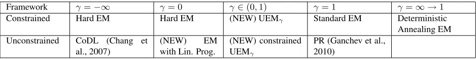
Table 1: Summary of different UEM algorithms. The entries marked with “(NEW)” have not been proposed before. Eq. (8) is the objective function for all the EM frameworks listed in this table. Note that, in the absence of constraints, γ∈(−∞,0]corresponds to hard EM (Sec. 3.1.1.) Please see Sec. 3.1 for a detailed explanation.

min q

P

h∈H(x)

γq(h) logq(h)−q(h) logPθ(h|x)(8)

s.t. Eq[Uh]≤b,

q(h)≥0,∀h∈ H(x),

P

h∈H(x)q(h) = 1 .

We discuss below, both the constrained and the unconstrained cases. Tab. 1 summarizes different EM algorithms in the UEM family.

3.1.1 UEM Without Constraints

The E-step in this case, computes a q obeying only the simplex constraints: P

h∈H(x)q(h) = 1.

For γ = 1, UEM minimizes KL(q, Pθ(h|x); 1) which is the same as minimizing KL(q, Pθ(h|x)) as in the standard EM (3). For γ = 0, UEM is solvingarg min_q∈Q

P

h∈H(x)−q(h) logPθ(h|x)

which is a linear programming (LP) problem. Due to the unimodularity of the simplex constraints (Schri-jver, 1986), this LP outputs an integral q =

δh= arg max_h∈H(x)Pθ(h|x)

which is the same as hard EM (4). It has already been noted in the liter-ature (Kearns et al., 1997; Smith and Eisner, 2004; Hofmann, 2001) that this formulation (correspond-ing to ourγ = 0) is the same as hard EM. In fact, for γ ≤ 0, UEM stays the same as hard EM be-cause of negative penalty on the entropy. The range

γ ∈ (0,1)has not been discussed in the literature, to the best of our knowledge. In Sec. 5, we show the impact of using UEMγfor γ ∈ {0,1}. Lastly, the range ofγ from∞to 1 has been used in deter-ministic annealing for EM (Rose, 1998; Ueda and Nakano, 1998; Hofmann, 2001). However, the focus of deterministic annealing is solely to solve the stan-dard EM while avoiding local maxima problems.

3.1.2 UEM With Constraints

UEM and Posterior Regularization (γ = 1) For

γ = 1, UEM solves arg min_q∈QKL(q, Pθ(h|x))

which is the same as Posterior Regulariza-tion (Ganchev et al., 2010).

UEM and CoDL (γ = −∞) When γ → −∞

then due to an infinite penalty on the entropy of the posterior, the entropy must become zero. Thus, now the E-step, as expressed by Eq. (8), can be written as

q=δ(h=h∗)whereh∗is obtained as

arg max

h∈H(x)

logPθ(h|x) (9)

s.t. Uh≤b ,

which is the same as CoDL. This combinatorial maximization can be solved using the Viterbi algo-rithm in some cases or, in general, using Integer Lin-ear Programming (ILP.)

3.2 UEM withγ ∈[0,1]

Tab. 1 lists different EM variations and their associ-ated valuesγ. This paper focuses on values ofγ be-tween 0 and 1 for the following reasons. First, the E-step (8) is non-convex forγ < 0and hence compu-tationally expensive; e.g., hard EM (i.e. γ =−∞) requires ILP inference. Forγ ≥ 0, (8) is a convex optimization problem which can be solved exactly and efficiently. Second, forγ = 0, the E-step solves

max q

P

h∈H(x)q(h) logPθ(h|x) (10)

s.t. Eq[Uh]≤b,

q(h)≥0,∀h∈ H(x),

P

h∈H(x)q(h) = 1 ,

which is an LP-relaxation of hard EM (Eq. (4) and (9)). LP relaxations often provide a decent proxy to ILP (Roth and Yih, 2004; Martins et al., 2009). Third,γ ∈[0,1]covers standard EM/PR.

3.2.1 Discussion: Role ofγ

KL(q, Pθ(y|x)) + (1−γ)H(q)— UEM (6) mini-mizes the former during the E-step, while Standard EM (3) minimizes the latter. The additional term

(1−γ)H(q)is essentially an entropic prior on the posterior distributionq which can be used to regu-larize the entropy as desired.

For γ < 1, the regularization term penalizes the

entropy of the posterior thus reducing the probability mass on the tail of the distribution. This is signifi-cant, for instance, in unsupervised structured predic-tion where the tail can carry a substantial amount of probability mass as the output space is massive. This notion aligns with the observation of (Spitkovsky et al., 2010) who criticize EM for frittering away too much probability mass on unimportant outputs while showing that hard EM does much better in PCFG parsing. In particular, they empirically show that when initialized with a “good” set of parame-ters obtained by supervised learning, EM drifts away (thus losing accuracy) much farther than hard-EM.

4 Solving Constrained E-step with Lagrangian Dual

In this section, we discuss how to solve the E-step (8) for UEM. It is a non-convex problem for

γ < 0; however, forγ =−∞(CoDL) one can use

ILP solvers. We focus here on solving the E-step for

γ ≥0for which it is a convex optimization problem, and use a Lagrange relaxation algorithm (Bertsekas, 1999). Our contributions are two fold:

• We describe an algorithm for UEM with con-straints that is as easy to implement as PR or CoDL. Existing code for constrained EM (PR or CoDL) can be easily extended to run UEM.

• We solve the E-step (8) using a Lagrangian dual-based algorithm which performs projected subgradient-ascent on dual variables. Our al-gorithm covers Lagrange relaxation and dual decomposition techniques (Bertsekas, 1999) which were recently popularized in NLP (Rush and Collins, 2011; Rush et al., 2010; Koo et al., 2010). Not only do we extend the algorithmic framework to a continuum of algorithms, we also allow, unlike the aforementioned works, general inequality constraints over the output variables. Furthermore, we establish new and

interesting connections between existing con-strained inference techniques.

4.1 Projected Subgradient Ascent with Lagrangian Dual

We provide below a high-level view of our algo-rithm, omitting the technical derivations due to lack of space. To solve the E-step (8), we introduce dual variablesλ— one for each expectation constraint in

Q. The subgradientOλof the dual of Eq. (8) w.r.t.

λis given by

Oλ∝Eq[Uh]−b . (11)

For γ > 0, the primal variableq can be written in

terms ofλas

q(h)∝Pθt(h|x)

1

γ_e− λTUh

γ _{. (12)}

For γ = 0, theq above is not well defined and so we take the limitγ → 0in (12) and sincelp norm approaches the max-norm asp→ ∞, this yields

q(h) =δ(h= arg max

h0_∈H(x)

Pθ(h0|x)e−λ

T_Uh0

). (13)

We combine both the ideas by setting q(h) =

G(h, Pθt(·|x), λTU, γ)where

G(h, P,v, γ) =

        

P(h) 1

γ_e−vhγ

P h0P(h0)

1

γe− vh0

γ

γ >0 ,

δ(h=arg max

h0∈H(x)

P(h0)e−vh0) γ= 0 .

(14)

Alg. 2 shows the overall optimization scheme. The dual variables for inequality constraints are re-stricted to be positive and hence after a gradient up-date, negative dual variables are projected to 0.

Note that forγ = 0, our algorithm is a Lagrange relaxation algorithm for approximately solving the E-step for CoDL (which uses exactarg max infer-ence). Lagrange relaxation has been recently shown to provide exact and optimal results in a large num-ber of cases (Rush and Collins, 2011). This shows that our range of algorithms is very broad — it in-cludes PR and a good approximation to CoDL.

Overall, the required optimization (8) can be solved efficiently if the expected value computation in the dual gradient (Eq. (11)) w.r.t. the posteriorq

Algorithm 2Solving E-step of UEMγforγ ≥0. 1: Initializeand normalizeq; initializeλ=0. 2: fort= 0, . . . , Ror until convergencedo

3: λ←max (λ+ηt(Eq[Uh]−b),0)

4: q(h) =G(h, Pθt(·|x), λTU, γ)

5: end for

can compute the posterior probability q explicitly using the dual variables. In cases where the out-put space is structured and exponential in size, e.g. word alignment, we can optimize (8) efficiently if the constraints and the model Pθ(h|x) decompose in the same way. To elucidate, we give a more con-crete example in the next section.

4.2 Projected Subgradient based Dual Decomposition Algorithm

Solving the inference (8) using Lagrangian dual can often help us decompose the problem into compo-nents and handle complex constraints in the dual space as we show in this section. Suppose our task is to predict two output variables h1 and h2

coupled via linear constraints. Specifically, they obey Ueh1 = Ueh2 (agreement constraints) and

Uih1 ≤ Uih2 (inequality constraints)4 for given matricesUeandUi. Let their respective probabilis-tic models beP_θ11 andP_θ22. The E-step (8) can be written as

arg min q1,q2

A(q1, q2;γ) (15)

s.t. Eq1[Ueh1] =Eq2[Ueh2]

Eq1[Uih1]≤Eq2[Uih2] ,

whereA(q1, q2;γ) = KL(q1(h1), P_θ11(h1|x);γ) +

KL(q2(h2), Pθ22(h2|x);γ).

The application of Alg. 2 results in a dual decom-position scheme which is described in Alg. 3.

Note that in the absence of inequality constraints and for γ = 0, our algorithm reduces to a simpler dual decomposition algorithm with agreement con-straints described in (Rush et al., 2010; Koo et al., 2010). Forγ = 1with agreement constraints, our algorithm specializes to an earlier proposed tech-nique by (Ganchev et al., 2008). Thus our algo-rithm puts these dual decomposition techniques with

4

The analysis remains the same for a more general formu-lation with a constant offset vector on the R.H.S. and different matrices forh1andh2.

Algorithm 3 Projected Subgradient-based Lagrange Relaxation Algorithm that optimizes Eq. (15)

1: Input:Two distributionsP1 θ1andP

2 θ2. 2: Output:Output distributionsq1andq2in (15)

3: DefineλT ₌

λeT λiT

andUT ₌

UeT UiT

4: λ←0

5: fort= 0, . . . , Ror until convergencedo

6: q1(h1)←G(h1, Pθ11(·|x), λ

T_{U, γ)}

7: q2(h2)←G(h2, Pθ22(·|x),−λ

T_{U, γ)}

8: λe←λe+ηt(−Eq1[Ueh 1_{] +E}

q2[Ueh 2_])

9: λi←λi+ηt(−Eq1[Uih 1_{] +E}

q2[Uih 2_])

10: λi←max(λi,0){Projection step}

11: end for

12: return (q1, q2)

agreement constraints on the same spectrum. More-over, dual-decomposition is just a special case of Lagrangian dual-based techniques. Hence Alg. 2 is more broadly applicable (see Sec. 5). Lines 6-9 show that the required computation is decomposed over each sub-component.

Thus if computing the posterior and expected val-ues of linear functions over each subcomponent is easy, then the algorithm works efficiently. Con-sider the case when constraints decompose linearly overhand each component is modeled as an HMM with θS as the initial state distribution, θE as em-mision probabilities, and θT as transition probabil-ities. An instance of this is word alignment over language pair(S, T) modeled using an HMM aug-mented with agreement constraints which constrain alignment probabilities in one direction (Pθ1: from

StoT) to agree with the alignment probabilities in the other direction (Pθ2: fromT toS.) The agree-ment constraints are linear over the alignagree-ments,h.

Now, the HMM probability is given by

Pθ(h|x) = θS(h0)QiθE(xi|hi)θT(hi+1|hi)

wherevi denotes theith component of a vector v.

For γ > 0, the resulting q (14) can be expressed

using a vectorµ=+/-λTU(see lines 6-7) as

q(h)∝ θS(h0)

Y

i

θE(xi|hi)θT(hi+1|hi) !γ1

e

P

i µihi γ

∝Y

i

θS(h0) 1

γ _θE(xi|_hi)eµihiγ1 _θ

T(hi+1|hi)

1

γ _.

θT to the power1/γand normalizing. Forγ = 0,q can be computed as the most probable output. The required computations in lines 6-9 can be performed using the forward-backward algorithm or the Viterbi algorithm. Note that we can efficiently compute ev-ery step because the linear constraints decompose nicely along the probability model.

5 Experiments

Our experiments are designed to explore tuning γ

in the UEM framework as a way to obtain gains over EM and hard EM in the constrained and uncon-strained cases. We conduct experiments on POS-tagging, word-alignment, and information extrac-tion; we inject constraints in the latter two. In all the cases we use our unified inference step to implement general UEM and the special cases of existing EM algorithms. Since both of our constrained problems involve large scale constrained inference during the E-step, we use UEM0 (with a Lagrange relaxation

based E-step) as a proxy for ILP-based CoDL . As we varyγ over[0,1], we circumvent much of the debate over EM vs hard EM (Spitkovsky et al., 2010) by exploring the space of EM algorithms in a “continuous” way. Furthermore, we also study the relation between quality of model initialization and the value ofγ in the case of POS tagging. This is inspired by a general “research wisdom” that hard EM is a better choice than EM with a good initial-ization point whereas the opposite is true with an “uninformed” initialization.

Unsupervised POS Tagging We conduct exper-iments on unsupervised POS learning experiment with the tagging dictionary assumption. We use a standard subset of Penn Treebank containing 24,115 tokens (Ravi and Knight, 2009) with the tagging dic-tionary derived from the entire Penn Treebank. We run UEM with a first order (bigram) HMM model5. We consider initialization points of varying quality and observe the performance forγ ∈[0,1].

Different initialization points are constructed as follows. The “posterior uniform” initialization is created by spreading the probability uniformly over all possible tags for each token. Our EM model on

5

(Ravi and Knight, 2009) showed that a first order HMM model performs much better than a second order HMM model on unsupervised POS tagging

-0.15 -0.1 -0.05 0 0.05

1.0 0.9 0.8 0.7 0.6 0.5 0.4 0.3 0.2 0.1 0.0

Relative performance to EM (Gamma=1)

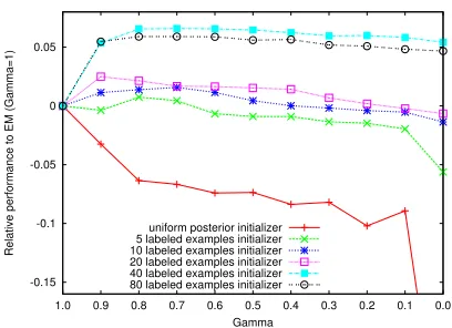
Gamma uniform posterior initializer 5 labeled examples initializer 10 labeled examples initializer 20 labeled examples initializer 40 labeled examples initializer 80 labeled examples initializer

Figure 1: POS Experiments showing the relation between initial model parameters andγ. We report the relative per-formance compared to EM (see Eq. (16)). The posterior uniform initialization does not use any labeled examples. As the no. of labeled examples used to create the initial HMM model increases, the quality of the initial model improves. The results show that the value of the bestγis sensitive to the initialization point and EM (γ = 1) and hard EM (γ= 0) are often not the best choice.

this dataset obtains 84.9% accuracy on all tokens and 72.3% accuracy on ambiguous tokens, which is competitive with results reported in (Ravi and Knight, 2009). To construct better initialization points, we train a supervised HMM tagger on hold-out labeled data. The quality of the initialization points is varied by varying the size of the labeled data over {5,10,20,40,80}. Those initialization points are then fed into different UEM algorithms.

Results For a particular γ, we report the perfor-mance of UEMγ w.r.t. EM (γ = 1.0) as given by

rel(γ) = Acc(UEMγ)−Acc(UEMγ=1.0)

Acc(UEMγ_=1.0)

(16)

whereAcc represents the accuracy as evaluated on the ambiguous words of the given data. Note that

rel(γ) ≷ 0, implies performance better or worse than EM. The results are summarized in Figure 1.

of γ, is closely related to the quality of the ini-tialization pointbut also elicit a more fine-grained relationship between initialization and UEM.

This experiment agrees with (Merialdo, 1994), which shows that EM performs poorly in the semi-supervised setting. In (Spitkovsky et al., 2010), the authors show that hard EM (Viterbi EM) works bet-ter than standard EM. We extend these results by showing that this issue can be overcome with the UEM framework by picking appropriateγbased on the amount of available labeled data.

Semi-Supervised Entity-Relation Extraction

We conduct semi-supervised learning (SSL) ex-periments on entity and relation type prediction assuming that we are given mention boundaries. We borrow the data and the setting from (Roth and Yih, 2004). The dataset has 1437 sentences; four entity types: PER, ORG, LOC, OTHERS and; five relation types LIVE IN, KILL, ORG BASED IN, WORKS FOR, LOCATED IN. We consider relations between all within-sentence pairs of entities. We add a relation type NONE indicating no relation exists between a given pair of entities.

We train two log linear models for entity type and relation type prediction, respectively via discrimina-tive UEM. We work in a discriminadiscrimina-tive setting in order to use several informative features which we borrow from (Roth and Small, 2009). Using these features, we obtain 56% average F1 for relations and 88% average F1 for entities in a fully supervised set-ting with an 80-20 split which is competitive with the reported results on this data (Roth and Yih, 2004; Roth and Small, 2009). For our SSL experiments, we use 20% of data for testing, a small amount,κ%, as labeled training data (we varyκ), and the remain-ing as unlabeled trainremain-ing data. We initialize with a classifier trained on the given labeled data.

We use the following constraints on the posterior. 1) Type constraints: For two entitiese1 ande2, the

relation typeρ(e1, e2)between them dictates a

par-ticular entity type (or in general, a set of entity types) for both e1 ande2. These type constraints can be

expressed as simple logical rules which can be con-verted into linear constraints. E.g. if the pair(e1, e2)

has relation type LOCATED INthene2must have

en-tity type LOC. This yields a logical rule which is converted into a linear constraint as

0.3   0.32   0.34   0.36   0.38   0.4   0.42   0.44   0.46   0.48  

5   10   20  

Av

g.

 F1

 fo

r  r

el

a5

on

s  

%  of  labeled  data  

Sup.  Bas.   PR  

CoDL   UEM  

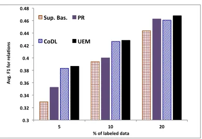
Figure 2: Average F1 for relation prediction for varying sizes of labeled data comparing the supervised baseline, PR, CoDL, and UEM. UEM is statistically significantly better than supervised baseline and PR in all the cases.

(ρ(e1, e2) ==LOCATED IN) → (e2 ==LOC) ⇒q(LOCATED IN;e1, e2) ≤ q(LOC;e2) .

Refer to (Roth and Yih, 2004) for more statistics on this data and a list of all the type constraints used. 2) Expected count constraints: Since most entity pairs are not covered by the given relation types, the presence of a large number of NONErelations can overwhelm SSL. To guide learning in the right direc-tion, we use corpus-wide expected count constraints for each non-NONErelation type. These constraints are very similar to thelabel regularizationtechnique mentioned in (Mann and McCallum, 2010). LetDr be the set of entity pairs as candidate relations in the entire corpus. For each non-NONErelation typeρ, we impose the constraints

Lρ≤

X

(e1,e2)∈Dr

q(ρ;e1, e2)≤Uρ ,

whereLρandUρare lower and upper bound on the expected number ofρrelations in the entire corpus. Assuming that the labeled and the unlabeled data are drawn from the same distribution, we obtain these bounds using the fractional counts ofρover the la-beled data and then perturbing it by +/- 20%.

value of gamma is 0.52, 0.6, and 0.57, respectively; the median values are 0.5, 0.6, and 0.5, respectively. For relation extraction, UEM is always statistically significantly better than the baseline and PR. The difference between UEM and CoDL is small which is not very surprising because hard EM approaches like CoDL are known to work very well for discrim-inative SSL. We omit the graph for entity predic-tion because EM-based approaches do not outper-form the supervised baseline there. However, no-tably, for entities, forκ = 10%, UEM outperforms CoDL and PR and for20%, the supervised baseline outperforms PR statistically significantly.

Word Alignment Statistical word alignment is a well known structured output application of unsu-pervised learning and is a key step towards ma-chine translation from a source languageS to a tar-get languageT. We experiment with two language-pairs: English-French and English-Spanish. We use Hansards corpus for French-English trans-lation (Och and Ney, 2000) and Europarl cor-pus (Koehn, 2002) for Spanish-English translation with EPPS (Lambert et al., 2005) annotation.

We use an HMM-based model for word-alignment (Vogel et al., 1996) and add agreement constraints (Liang et al., 2008; Ganchev et al., 2008) to constrain alignment probabilities in one direction (Pθ1: fromStoT) to agree with the alignment prob-abilities in the other direction (Pθ2: fromT to S.) We use a small development set of size 50 to tune the model. Note that the amount of labeled data we use is much smaller than the supervised approaches reported in (Taskar et al., 2005; Moore et al., 2006) and unsupervised approaches mentioned in (Liang et al., 2008; Ganchev et al., 2008) and hence our results are not directly comparable. For the E-step, we use Alg. 3 with R=5 and pickγfrom{0.0,0.1, . . . ,1.0}, tuning it over the development set.

During testing, instead of running HMM mod-els for each direction separately, we obtain posterior probabilities by performing agreement constraints-based inference as in Alg. 3. This results in a posterior probability distribution over all possible alignments. To obtain final alignments, follow-ing (Ganchev et al., 2008) we use minimum Bayes risk decoding: we align all word pairs with poste-rior marginal alignment probability above a certain

Size EM PR CoDL UEM EM PR CoDL UEM

En-Fr Fr-En

10k 23.54 10.63 14.76 9.10 19.63 10.71 14.68 9.21

50k 18.02 8.30 10.08 7.34 16.17 8.40 10.09 7.40

100k 16.31 8.16 9.17 7.05 15.03 8.09 8.93 6.87

En-Es Es-En

10k 33.92 22.24 28.19 20.80 31.94 22.00 28.13 20.83

50k 25.31 19.84 22.99 18.93 24.46 20.08 23.01 18.95

100k 24.48 19.49 21.62 18.75 23.78 19.70 21.60 18.64

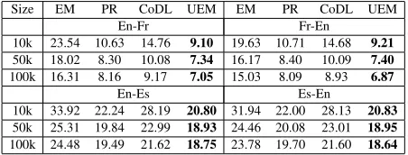
Table 2: AER (Alignment Error Rate) comparisons for French-English (above) and Spanish-English (below) alignment for various data sizes. For French-English set-ting, tunedγ for all data-sizes is either 0.5 or 0.6. For Spanish-English, tunedγfor all data-sizes is 0.7.

threshold, tuned over the development set.

Results We compare UEM with EM, PR, and CoDL on the basis of Alignment Error Rate (AER) for different sizes of unlabeled data (See Tab. 2.) See (Och and Ney, 2003) for the definition of AER. UEM consistently outperforms EM, PR, and CoDL with a wide margin.

6 Conclusion

We proposed a continuum of EM algorithms parameterized by a single parameter. Our frame-work naturally incorporates constraints on output variables and generalizes existing constrained and unconstrained EM algorithms like standard and hard EM, PR, and CoDL. We provided an efficient Lagrange relaxation algorithm for inference with constraints in the E-step and empirically showed how important it is to choose the right EM version. Our technique is amenable to be combined with many existing variations of EM (Berg-Kirkpatrick et al., 2010). We leave this as future work.

References

K. Bellare, G. Druck, and A. McCallum. 2009. Alter-nating projections for learning with expectation con-straints. InUAI.

T. Berg-Kirkpatrick, A. Bouchard-Cˆot´e, J. DeNero, and D. Klein. 2010. Painless unsupervised learning with features. InACL, HLT ’10.

D. P. Bertsekas. 1999. Nonlinear Programming. Athena Scientific, 2nd edition.

P. Brown, S. D. Pietra, V. D. Pietra, and R. Mercer. 1993. The mathematics of statistical machine translation: pa-rameter estimation. Computational Linguistics. M. Chang, L. Ratinov, and D. Roth. 2007. Guiding

semi-supervision with constraint-driven learning. InACL. J. Clarke and M. Lapata. 2006. Constraint-based

sentence compression: An integer programming ap-proach. InACL.

A. P. Dempster, N. M. Laird, and D. B. Rubin. 1977. Maximum likelihood from incomplete data via the EM algorithm. Journal of the Royal Statistical Society. K. Ganchev, J. Graca, and B. Taskar. 2008. Better

align-ments = better translations. InACL.

K. Ganchev, J. Grac¸a, J. Gillenwater, and B. Taskar. 2010. Posterior regularization for structured latent variable models. Journal of Machine Learning Re-search.

T. Hofmann. 2001. Unsupervised learning by probabilis-tic latent semanprobabilis-tic analysis. MlJ.

M. Kearns, Y. Mansour, and A. Y. Ng. 1997. An information-theoretic analysis of hard and soft assign-ment methods for clustering. InICML.

D. Klein and C. D. Manning. 2004. Corpus-based induc-tion of syntactic structure: models of dependency and constituency. InACL.

P. Koehn. 2002. Europarl: A multilingual corpus for evaluation of machine translation.

T. Koo, A. M. Rush, M. Collins, T. Jaakkola, and D. Son-tag. 2010. Dual decomposition for parsing with non-projective head automata. InEMNLP.

P. Lambert, A. De Gispert, R. Banchs, and J. Marino. 2005. Guidelines for word alignment evaluation and manual alignment. Language Resources and Evalua-tion.

P. Liang, D. Klein, and M. I. Jordan. 2008. Agreement-based learning. InNIPS.

G. S. Mann and A. McCallum. 2010. Generalized expectation criteria for semi-supervised learning with weakly labeled data. JMLR, 11.

A. Martins, N. A. Smith, and E. Xing. 2009. Concise integer linear programming formulations for depen-dency parsing. InACL.

A. K. McCallum, R. Rosenfeld, T. M. Mitchell, and A. Y. Ng. 1998. Improving text classification by shrinkage in a hierarchy of classes. InICML.

B. Merialdo. 1994. Tagging text with a probabilistic model. Computational Linguistics.

R. C. Moore, W. Yih, and A. Bode. 2006. Improved discriminative bilingual word alignment. InACL. R. M. Neal and G. E. Hinton. 1998. A new view of

the EM algorithm that justifies incremental, sparse and other variants. In M. I. Jordan, editor, Learning in Graphical Models.

K. Nigam, A. K. Mccallum, S. Thrun, and T. Mitchell. 2000. Text classification from labeled and unlabeled documents using EM.Machine Learning.

F. J. Och and H. Ney. 2000. Improved statistical align-ment models. InACL.

F. J. Och and H. Ney. 2003. A systematic comparison of various statistical alignment models. CL, 29.

S. Ravi and K. Knight. 2009. Minimized models for unsupervised part-of-speech tagging. ACL, 1(August). K. Rose. 1998. Deterministic annealing for clustering, compression, classification, regression, and related op-timization problems. InIEEE, pages 2210–2239. D. Roth and K. Small. 2009. Interactive feature space

construction using semantic information. In Proc. of the Annual Conference on Computational Natural Language Learning (CoNLL).

D. Roth and W. Yih. 2004. A linear programming formu-lation for global inference in natural language tasks. In H. T. Ng and E. Riloff, editors,CoNLL.

D. Roth and W. Yih. 2007. Global inference for entity and relation identification via a linear programming formulation. In L. Getoor and B. Taskar, editors, In-troduction to Statistical Relational Learning.

A. M. Rush and M. Collins. 2011. Exact decoding of syntactic translation models through lagrangian relax-ation. InACL.

A. M. Rush, D. Sontag, M. Collins, and T. Jaakkola. 2010. On dual decomposition and linear program-ming relaxations for natural language processing. In

EMNLP.

A. Schrijver. 1986. Theory of linear and integer pro-gramming. John Wiley & Sons, Inc.

N. A. Smith and J. Eisner. 2004. Annealing techniques for unsupervised statistical language learning. InACL. V. I. Spitkovsky, H. Alshawi, D. Jurafsky, and C. D. Man-ning. 2010. Viterbi training improves unsupervised dependency parsing. InCoNLL.

B. Taskar, S. Lacoste-Julien, and D. Klein. 2005. A dis-criminative matching approach to word alignment. In

HLT-EMNLP.