Wavelet Lifting over Information-Based EEG Graphs for Motor Imagery Data Classification

Wavelet lifting over information-based EEG graphs for

motor imagery data classification

Javier Asensio-Cubero1, John Q. Gan1, and Ramaswamy Palaniappan2 1 _{University of Essex,Wivenhoe Park, Colchester, Essex CO4 3SQ,United Kingdom}

[email protected], [email protected]

2 _{University of Wolverhampton, Shifnal Road, Telford, TF2 9NT, United Kingdom} [email protected]

Abstract. The imagination of limb movements offers an intuitive paradigm for the control of electronic devices via brain computer interfacing (BCI). The anal-ysis of electroencephalographic (EEG) data related to motor imagery potentials has proved to be difficult task. EEG readings are noisy, and the elicited patterns occur in different parts of the scalp, at different instants and at different frequen-cies. Wavelet transform has been widely used in the BCI field as it offers temporal and spectral capabilities, although it lacks of spatial information. In this study we propose the use of a tailored second generation wavelet to extract features from these three domains. This transform is applied over a graph representation of mo-tor imaginary trials, which encodes temporal and spatial information. This graph is enhanced using per-subject knowledge in order to optimise the spatial rela-tionships among the electrodes, and to improve the filter design. The resulting method improves the performance of classifying different imaginary limb move-ments maintaining the low computational resources required by the lifting trans-form over graphs. By using an online dataset we were able to positively assess the feasibility of using the novel method in online BCI contexts.

1

Introduction

Brain signal analysis, applied for the control of computerised devices, deter-mines a human-machine interaction paradigm known as brain-computer interfac-ing (BCI). This new way of communication not only has a direct positive impact on motor disabled users in terms of quality of life and interaction with their sur-roundings, but also opens new modes of operation for healthy users to interact with their environment.

The human brain responds to different stimuli with alterations in its neural activ-ity. These alterations which manifest as changes in the electrical activity in the cortex and changing blood oxygen levels in different regions, can be measured with appropriate technology. In terms of electrical activity, these responses pro-voke oscillations known as event related potentials (ERP) that can be measured with electroencephalographic (EEG) devices and detected with appropriate algo-rithms [11].

One example of an ERP is the imagination of limb movements, which is com-monly known as motor imagery (MI). Depending on the limb involved, the brain activity derived from MI tasks produces changes in neural activity on different parts of the brain cortex, at different rates and with different temporal behaviour.

These changes produce a series of short lasting amplifications and attenuations in the EEG data known as event related desynchronisation (ERD) and event related synchronisation (ERS) [17].

The study of ERS/ERD has proven to be a hard task. EEG data is noisy and of low amplitude, there is no inter-subject pattern consistency, and features that make the ERS/ERD patterns recognisable appear at different time intervals, different scalp locations and different frequency bands.

Wavelets have been profusely applied in the BCI domain as they allow a meaning-ful temporal-spectral analysis of the EEG data. Shifts and dilations of a mother wavelet function provide a series of orthogonal subspaces resulting in what is known as multi-resolution analysis (MRA) [10]. First generation wavelets present a major disadvantage of difficult design. Researchers usually make use of well established wavelet families, even though the wavelet function features may not completely fulfil the needs of the domain of study.

On the other hand, during the last decade a new wavelet framework has become popular for building tailored wavelets. Wavelet lifting, often referred to as second generation wavelets, offers a simple framework to construct wavelet functions that have fewer restrictions and can be applied in a natural way to many situations that first generation wavelets are incapable of handling [23] [24].

The possibilities offered by the lifting transform open new interesting ways to look at BCI signal processing. In [1] a new MRA system for BCI data anal-ysis was proposed using lifting scheme over graphs to fully explore the three domains involved in ERS/ERD patterns evolution. Graph EEG data representa-tion is a natural way of describing the spatio/temporal relarepresenta-tions among electrode readings. The purpose of this study is to extend the static graph representation by automatically building an enhanced graph in which the connections represent meaningful relationships among different electrodes. For this purpose we used mutual information as it provides a measurement of how much information one channel shares with another channel.

The paper is organised as follows: data acquisition is detailed in Section 2.1, Sec-tion 2.2 explains the lifting scheme over graphs, SecSec-tion 2.3 describes how the graphs are built, Section 2.4 focuses on the feature extraction technique, pattern description and classification methods, and the experimental methodology is de-scribed in Section 2.5. The obtained results along with discussions are presented in Section 3. Finally, the conclusions are drawn in Section 4.

2

Methods

2.1 Data Acquisition and Preprocessing

The first dataset was recorded at the BCI Laboratory at the University of Essex. The protocol was set up as follows: The electrode placement followed the 10-20 international system and 32 channels were recorded with a sampling frequency of 256 Hz. During the recording session the subject was sitting on an arm-chair in front of a computer screen. A fixation cross was showed at the beginning of the trial att=0s. Att=2sa cue was shown indicating the imaginary movement class to perform. The end of the trial was marked when the fixation cross and cue disappeared att=8s. The subjects were asked to perform 120 trials of each of the three imaginary movements (right hand, left hand and feet). A total of 12

subjects participated in the recording sessions, half of them were naive on the use of BCI systems, 58% of the subjects were female, and the ages ranged from 24 to 50. During the result analysis these subjects were identified by the prefixE-X, withXbeing the subject number.

The second dataset is from the BCI Competition IV (dataset 2a) and follows a similar acquisition protocol. The full experiment description can be found in [5]. The data covers four different types of MI movement data: right-hand, left-hand, feet and tongue recorded at 250Hz. There are a total of 288 trials recorded, for each of the nine subjects. The subjects belonging to this dataset are identified by the prefixC-X.

The calibration trials of the third dataset were acquired following an identical pro-tocol to the one described for the first dataset. The validation trials were recorded while the subject controlled a BCI system in real-time with continuous feedback, even though the results for the online classification are not the ones described here, the data was reprocessed for this study. Twelve healthy subjects took part in the experiment, all of whom were naive to the use of online BCI. The subjects were aged from 24 to 32 and 50% were female. The results for this dataset are labeled with the prefixO-X.

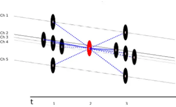
Fig. 1: Numbering of the 15 electrodes used during the experimentation, which were allocated from FC3 to FC4, C3 to C4, and CP3 to CP4.

For this study we utilised a subset of 15 electrodes, covering the major area of the motor cortex ( Figure 1). The original data was filtered from 8 to 30 Hz in order to attenuate external noise and artifacts. Each trialXiofTsamples was scaled by

applyingXi=√1_TXiorig(It−1t1

0

t), whereItis theT×T identity matrix and 1tis

aT dimensional vector with ones in it.

The competition data was already divided into training and evaluation subsets. The off-line data from the University of Essex was split using the first two ac-quisition runs (180 trials) as training data and the last two runs (180 trials) as evaluation set. The data from the online experiment contained 160 trials for cali-bration and 90 trials for validation purposes.

2.2 Wavelet Lifting over EEG Graphs

First generation wavelets represent signals in terms of shifts and dilations of the basis function known as mother wavelet. The design of this function obeys a set of restrictions assuring an accurate orthogonal decomposition of the original data. The main benefit of wavelet analysis over other orthogonal systems, such as the Fourier transform or the cosine transform, is its multiscale capability. Wavelets allow to analyse the data not only in the frequency domain, but also in the tem-poral domain at different levels. [10] [12].

The use of first generation wavelets is pervasive in many domains where signal processing is involved, and BCIs are no exception.

In P-300 based BCIs is common to find wavelet decomposition used as method of signal analysis. In [4] they use non-parametric statistics from the different levels of a Mexican hat common wavelet transform. The Daubechies wavelet in its discrete variant was applied in [16] using the thresholded coefficients as feature vectors for classification.

There are also several examples of the use of the wavelet transform in MI-based BCIs. In [18] Morlet wavelets are used to decompose signals of imaginary limb movements. In [6] discrete wavelet transform is applied using different families (Daubechies, Coiflets and Symlets), sub-band power and the standard deviation of the analysis and detail coefficients at different levels are used as feature extraction method. In [26] Coiflet decompositions of fifth order are used, as they claim that its shape is the closest to the ERD/ERS signals.

It is rarer to find the wavelet transform in the study of SSVEP BCIs but it has been applied, as in [25] where continuous Morlet wavelets were used to study the EEG data.

One major issue to cope with when working with the wavelet transform is that wavelet function design is an extremely complex task, and therefore, researchers apply common families in their studies despite the mother wavelet may not be suitable for the domain of study. The introduction of second generation wavelets, also known as wavelet lifting [22], alleviates this problem making the design of complete multiresolution systems more straight forward. The wavelet lifting is capable of handling data where Fourier analysis is not suitable (and therefore first generation wavelets either) such as unevenly sampled data, surfaces, spheres [20], trees [21] and graphs [14] [13].

A lifting scheme consists of iterations of three basic operations [7]:

– Split:Separate the original signalxinto two subsets, referred as odd (xo)

and even (xe) elements.

– Predict:The error of predictingxoin base ofxeusing apredictor operator

P

– Update:The coarser approximation of the original signal is calculated by combiningxeanddusing anupdate operator

U

A lifting transform over graphs can be defined as follows [14]. Let us consider a graphG= (V,E)whereV is the node set of sizeN=No+NeandEthe edges

linking those nodes.Vis divided into the even and odd sets andEis represented using the adjacency matrixAd j. We rearrangeV andAd jso that the odd set of nodes (a vectorVoof sizeNo×1) is gathered before the even set (a vectorVeof

˜ V =Vo Ve ˜ Ad j= F No×No_JNo×Ne KNe×No_LNe×Ne ! (1) The submatricesF andLinAd j˜ in Equation (1) are discarded as they link ele-ments within the same node sets. The block matricesJandKcontain only edges linking nodes from different node sets.

The lifting transform functions are defined using a weighted version of the block matricesJandK:

D=Vo−Jω×Ve

A=Ve+Kω×D (2)

where the prediction and update functions are defined as a matrix product:

P

eand

U

matrices and their actual values depend on the domain of application.

We repeat the process described in Equation(2) in each levell+1 assigning the approximation coefficientsAin levelltoV.

2.3 Automatic EEG Graph Building and Filter Design

In [1], a static EEG data graph representation was introduced. This representation had the benefit of keeping a channel oriented structure although no extra infor-mation was used to optimise the inter-channel links. In order to stablish which channels should be connected for each subject we made use of the mutual infor-mation of every pair of channels [9][15].

Mutual information measures the amount of information that one random variable

Y contains about another random variableZand is given by:

I(Y;Z) =

_∑

∑

p(y,z)log p(y,z)

p(y)p(z) (3)

where p(y,z)is the joint probability mass function and, p(y) and p(z)is the marginal probability mass function.

Consider a set of MI trialsXT×CofT samples andCchannels. In order to sta-blish the relationships among the spatial locations we compute the mutual infor-mationM(r,s) =I(cr;cs)for every pair of channelscrcswithr∈ {1. . .C}and s∈ {1. . .C}. Note that the diagonal elements ofMare set to zero (the mutual information of a channel with itself is ignored) and rest of non-zero elements normalised between zero and one.

The symmetric matrixMdescribes how all the channels are related to each other and this information can be used to build a specific graph representation for each subject.

Let us assume that the graphGx= (Vx,Ex)is embedding a trialX, whereVx

defines the nodes and the edge setEx is represented by a weighted adjacency matrixAd jx:

Ad jxi j=

(

ai j Ifvxiis connected tovxj

For convenience, the odd set will correspond to the elements ofX at odd values oft, and the even set at even values oft. Therefore, we obtain two different node vectorsvxoandvxe.

Thepredictandupdatefilters are computed in terms of the matricesMandAd jx. The following steps are carried out in order to set the adjacency matrix values:

1. Apply a thresholdthto the matrixMsuch thatM(r,s) =0 ifM(r,s)<th, so only those channels with high mutual information values will be linked, and normalise the non-zero values between zero and one.

2. SetAd jx_{such that for a given channelcand instanttit will be connected to}

the previoust−1 and followingt+1 time instants with a weightai j=1.

3. For all the other channelscrand adjacent temporal valuest+1 andt−1 set

the weightai j=M(c,cr)in the corresponding entry ofAd jx, ifM(c,cr)>0.

The resulting adjacency submatrices ofFx_andLx_{fromAd j}x_{are empty. The} pre-dictandupdatematricesJωxandKωx(weighted versions the submatricesJxand

Kx) are computed row-wise asJ_{i j}ωx= J x i j ∑Jk=0Jikx andK_{i j}ωx= J x i j 2∗∑Jk=0Jikx . It is notewor-thy to mention that the obtained lifting filters are weighted Laplacian graph filters, and the design explained here ensures that those channels that share high mutual information will contribute more to the detail coefficients than those that share low mutual information.

2.4 Feature Extraction and Classification

One of the main drawbacks in the use of multiresolution analysis for signal classi-fication is the large number of coefficients generated during the transform. In or-der to overcome this problem we use common spatial patterns (CSP) as a method for feature extraction and dimensionality reduction. CSP is an extension to PCA where two different classes of data are taken into account.

Assuming that the trials contains data from the label (+) and the label (-), the set of samplesXis divided intoX(+)andX(−). Their simultaneously estimated covariance matrix decomposition is given by [3]:

Σ(+)=WΛ(+)WT

Σ(−)=WΛ(−)WT (5)

whereΣ(+)is the estimated covariance matrix for the trials belonging to class (+)

andΣ(−) is the covariance matrix for the trials belonging to class (-).Λ(+)and

Λ(−)are diagonal matrices with the eigenvalues corresponding to the decompo-sition ofΣ(+) andΣ(−). A large eigenvalueΛ(+)_{j j} means that the corresponding eigenvector from matrixW,wj, leads to high variance in the projected signal in

the positive class and low variance in the negative one (and vice-versa). The CSP projection results inYi=WTXi.

The different detailDl and approximationAlsets at different levelslfrom the MRA were projected onto their own CSP subspacesYDl_=WT

Dl×DlandYAl= W_ATl×Al. For clarity, we will refer toYDl andYAl using ¯Y.

For every ¯Y, we extracted the rows which maximised and minimised the vari-ance between the two different classes (namely, the firstmrows and lastmrows) and calculated every feature as fk=var(y¯k)withk={1,2, . . . ,m,C−m,C−

the difference among the feature values, the logarithm f_klog=log( fk ∑Fj=1fj)was

computed [19].

For this study,m∈2,3,4 was chosen using cross validation as explained in Sec-tion 2.5.

The features obtained from the CSP were classified using LDA as it provides a fair compromise between resource consumption and classification performance [2]. In order to measure the classification performance Kappa value [8] was used instead of the classification ratio. Kappa value gives an accurate description of the classifier’s performance, taking into account the per class error distribution. The Kappa value was computed asκ=p₁o₋−_ppc

c , wherepois the proportion of units

on which the judgement agrees (based on the output from the classifier and the actual label), andpcis the proportion of units on which the agreement is expected

by chance.

2.5 Experimental Methodology

After the data preprocessing, a temporal sliding window of one second with a fifth of second overlap was applied over each trial. The segmented data was then trans-formed using a lifting scheme over graphs (See Section 2.2 and Section 2.3) to the sixth level. The transformation resulted in twelve different coefficient sets, which were further processed to obtain the feature sets by selecting different number of CSP features (See Section 2.4).

The MRA approaches used for comparison were:

– Graph lifting scheme with static graphs [1]. The static graph is built by link-ing the elements from the surroundlink-ing channels as shown in Figure 2. The filters are calculated analogously as explained in Section 2.3 but by setting the weights of the Laplacian filters to one.

Fig. 2: Detail of the graph after the even/odd split for the static approach. The even element (in red) is linked to the surrounding odd elements (in black) adding spatial information to the decomposition.

– Graph lifting scheme and mutual information driven graph building. Each detail and approximation coefficient sets from the different temporal seg-ments were classified with a separate LDA model after applying CSP. This led to a total ofns∗l∗2 LDA outputs, withnsbeing the number of segments andlthe

number of levels. A majority voting approach was carried out in order to obtain the final classification output for each trial.

A cross-validation step using five folds was performed over the training data in or-der to select the two free parameters involved: the threshold applied to the mutual information matrix in Section 2.3 and the number of CSP features as explained in Section 2.4.

3

Results and Discussion

From the analysis of the mutual information matrixMfor the different subjects we learn that, in general, the standard deviations of the paired calculation do not differ much when compared among classes (two orders of magnitude smaller than the mean). Therefore, instead of computing a matrixMand a different graph to process one class against the others, we just use the whole set of data to generate the mutual information based adjacency matrix. This simplifies the model de-creasing the execution time. It is also noteworthy that the performance of the transform calculation does not vary although the values of the filters applied changed.

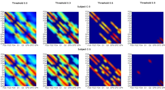
Fig. 3: Representation of the values ofMfor subjects C-3 and C-5 applying different thresholds

Figure 3,Figure 4 and Figure 5 are graphical representations of the values of the matrixM for different users and with different thresholds. In Figure 3 we find two examples to show that there exists a clear correlation between the electrode spatial location and the mutual information, the parallel lines crossing the fig-ure diagonally corresponds to high mutual information values between adjacent

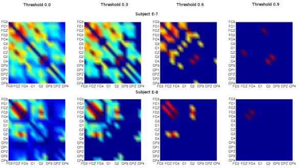
Fig. 4: Representation of the values of matrix M for subjects E-7 and E-8 applying different thresholds

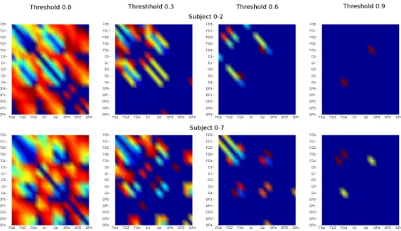
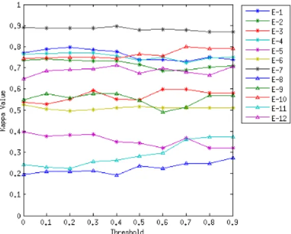
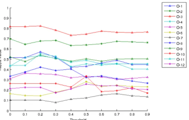
electrodes. This correlation is more evident if we compare it with with Figure 6, which corresponds to the matrixMof the static approach. Although from Fig-ure 4 to 5 this effect is still noticeable, it is more obvious how, for these specific subjects, the inter-electrode information is more prominent in particular locations of the motor cortex, concretely, in the frontal and central lobes for subject E-7 and 0-2, eminently central for subject E-8, and more scattered for subject 0-7. After applying the experimental methodology described in Section 2.5 we can analyse the impact of the automatic graph building on the classification results. Figure 7, Figure 8 and Figure 9 show how the median Kappa values change when different threshold values are applied. It is clear that the behaviour of the method is dependant on the subject of analysis. Some subjects, such as E-8, 4 and C-2, are not significantly affected by the change of the threshold value, although, on the other hand, we find subjects where the Kappa value fluctuates around 0.1 depending on the threshold value such as in subjects C-3, C-7, E-9, E-11, O-1 and O-4.

After selecting the two parameters, the mutual information threshold and the number of features used in CSP, from the cross-validation results we can com-pute the classification performance on the evaluation data. Table 1 shows the Kappa values and mean accuracy for the Essex dataset, Table 2 for the competi-tion dataset, and Table 3 for the online dataset.

For 78.8% of the 32 subjects the proposed method achieved a higher Kappa value. For some of the subjects this improvement rises the Kappa value by 0.1 when compared to the static approach.

Fig. 5: Representation of the values of matrixM for subjects O-2 and O-7 applying different thresholds

Fig. 6: Values of the matrixMfor the static graph approach.

There exists a difference between the Essex and the online datasets in terms of classification accuracy, even though the acquisition protocol was practically iden-tical. This decrement in the classification performance is due to effect of stress suffered by the subjects during the online experiments.

As a final remark we can mention that the proposed method obtains a Kappa value of 0.586 using the competition dataset, while the winner achieved 0.57.

Fig. 7: Median of the Kappa value in function of the threshold applied to the matrixMfor the competition dataset

Fig. 8: Median of the Kappa value in function of the threshold applied to the matrixMfor the Essex dataset

The small number of subjects in the competition data does not allow us to carry out a definitive significance test to compare both approaches.

4

Conclusions

In this study we have proposed a novel method to improve the EEG data rep-resentation based on static graphs by using the mutual information among the different channels, which constitutes an example of the possibilities offered by second generation wavelets in the BCI domain. This new strategy for building

Table 1: Results on the Essex dataset in terms of Kappa values. The mean accuracy is included at the bottom.

Subject GLS GLS + Mutual Information E-1 0.757 0.741 E-2 0.736 0.744 E-3 0.539 0.644 E-4 0.730 0.712 E-5 0.392 0.393 E-6 0.529 0.488 E-7 0.883 0.891 E-8 0.210 0.263 E-9 0.565 0.581 E-10 0.757 0.774 E-11 0.237 0.321 E-12 0.648 0.707 Mean Kappa 0.582 0.605 ± ± 0.21 0.19 Mean Acc 0.723 0.737 ± ± 0.14 0.13

Table 2: Results on the competition dataset in terms of Kappa values. The mean accuracy is included at the bottom.

Subject GLS GLS + Mutual Information

C-1 0.754 0.763 C-2 0.410 0.419 C-3 0.800 0.805 C-4 0.484 0.475 C-5 0.243 0.257 C-6 0.317 0.364 C-7 0.629 0.758 C-8 0.661 0.707 C-9 0.698 0.721 Mean Kappa 0.555 0.586 ± ± 0.19 0.20 Mean Acc 0.666 0.689 ± ± 0.15 0.15

Fig. 9: Median of the Kappa value in function of the threshold applied to the matrixMfor the online dataset

the graph also has an impact on the filter design, allowing an automatic way to weight the contribution of the different spatial locations.

After applying the proposed methodology on the three datasets, the resulting Kappa value was increased for an 78.8% percent of the subjects obtaining for several subjects an improvement of 0.1.

From the results achieved on the online dataset we can state that the proposed method is suitable for it use in online BCI systems, although the calibration time needed to obtain competitive results is relatively high, as the number of features used by CSP and the threshold have to be set via cross-validation.

Comparing the mutual information matrices from different subjects we can ob-serve how the initial static graph approach, where the surrounding electrodes were linked together, was appropriate as close electrodes tend to share similar informa-tion.

These positive results encourage us to explore new ways for optimising the graph representation of EEG data. Although mutual information has helped to improve the classification rate, other techniques such as Granger causality, which could be more robust when coping with non-stationarity, should be examined in future work.

Acknowledgements

The first author would like to thank the EPSRC for funding his Ph.D. study via an EPSRC DTA award.

References

1. Asensio-Cubero, J., Gan, J.Q., Palaniappan, R.: Multiresolution analysis over simple graphs for brain computer interfaces. Journal of Neural Engi-neering 10(4), 046014 (2013)

Table 3: Results on the online dataset in terms of Kappa values. The mean accuracy is included at the bottom.

Subject GLS GLS + Mutual Information O-1 0.494 0.454 O-2 0.640 0.711 O-3 0.777 0.789 O-4 0.432 0.541 O-5 0.334 0.376 O-6 0.306 0.278 O-7 0.107 0.165 O-8 0.248 0.376 O-9 0.534 0.504 O-10 0.222 0.320 O-11 0.434 0.532 O-12 0.179 0.263 Mean Kappa 0.392 0.443 ± ± 0.18 0.17 Mean Acc 0.59 0.629 ± ± 0.12 0.11

2. Blankertz, B., Muller, K.R., Krusienski, D.J., Schalk, G., Wolpaw, J.R., Schlogl, A., Pfurtscheller, G., Millan, J.R., Schroder, M., Birbaumer, N.: The BCI competition III: validating alternative approaches to actual BCI prob-lems. IEEE Transactions on Neural Systems and Rehabilitation Engineering 14(2), 153–159 (2006)

3. Blankertz, B., Tomioka, R., Lemm, S., Kawanabe, M., Muller, K.R.: Opti-mizing spatial filters for robust EEG single-trial analysis. IEEE Signal Pro-cessing Magazine 25(1), 41–56 (2008)

4. Bostanov, V.: BCI competition 2003-data sets ib and IIb: feature extraction from event-related brain potentials with the continuous wavelet transform and the t-value scalogram. IEEE Transactions on Biomedical Engineering 51(6), 1057–1061 (2004)

5. Brunner, C., Leeb, R., Muller-Putz, G.R., Schlogl, A., Pfurtscheller, G.: BCI competition 2008 - Graz data set A.http://www.bbci.de/competition/ iv/desc_2a.pdf(2008)

6. Carrera-Leon, O., Ramirez, J.M., Alarcon-Aquino, V., Baker, M. D’Croz-Baron, D., Gomez-Gil, P.: A motor imagery BCI experiment using wavelet analysis and spatial patterns feature extraction. In: 2012 Workshop on Engi-neering Applications (WEA). pp. 1–6 (2012)

7. Claypoole Jr, R.L., Baraniuk, R.G., Nowak, R.D.: Adaptive wavelet trans-forms via lifting. In: Proceedings of IEEE International Conference on Acoustics, Speech and Signal Processing. vol. 3, pp. 1513–1516 (1998) 8. Cohen, J.: A coefficient of agreement for nominal scales. Educational and

9. Cover, T.M., Thomas, J.A.: Elements of Information Theory. John Wiley & Sons (2012)

10. Daubechies, I.: Ten Lectures on Wavelets. Society for Industrial and Applied Mathematics (2006)

11. Dornhege, G.: Toward Brain-Computer Interfacing. The MIT Press (2007) 12. Mallat, S.G.: A theory for multiresolution signal decomposition: The wavelet

representation. IEEE Transactions on Pattern Analysis and Machine Intelli-gence. 11(7), 674–693 (1989)

13. Martinez-Enriquez, E., Ortega, A.: Lifting transforms on graphs for video coding. In: Data Compression Conference. pp. 73–82. IEEE (2011) 14. Narang, S.K., Ortega, A.: Lifting based wavelet transforms on graphs. In:

Conference of Asia-Pacific Signal and Information Processing Association. pp. 441–444 (2009)

15. Peng, H., Long, F., Ding, C.: Feature selection based on mutual informa-tion criteria of max-dependency, max-relevance, and min-redundancy. IEEE Transactions on Pattern Analysis and Machine Intelligence 27(8), 1226– 1238 (2005)

16. Perseh, B., Sharafat, A.R.: An efficient P300-based bci using wavelet fea-tures and IBPSO-based channel selection. Journal of Medical Signals and Sensors 2(3), 128 (2012)

17. Pfurtscheller, G., Lopes da Silva, F.H.: Event-related EEG/MEG synchro-nization and desynchrosynchro-nization: basic principles. Clinical Neurophysiology 110(11), 1842–1857 (1999)

18. Qin, L., He, B.: A wavelet-based timefrequency analysis approach for clas-sification of motor imagery for braincomputer interface applications. Journal of Neural Engineering 2, 65 (2005)

19. Ramoser, H., Muller-Gerking, J., Pfurtscheller, G.: Optimal spatial filtering of single trial EEG during imagined hand movement. IEEE Transactions on Rehabilitation Engineering 8(4), 441–446 (2000)

20. Schrder, P., Sweldens, W.: Spherical wavelets: Efficiently representing func-tions on the sphere. In: Proceedings of the 22nd Annual Conference on Com-puter Graphics and Interactive Techniques. pp. 161–172. ACM (1995) 21. Shen, G., Ortega, A.: Comopact image representation using wavelet lifting

along arbitrary trees. In: 15th IEEE International Conference on Image Pro-cessing, 2008. ICIP 2008. pp. 2808–2811. IEEE (2008)

22. Sweldens, W.: Wavelets and the lifting scheme: A 5 minute tour. Zeitschrift fur Angewandte Mathematik und Mechanik 76(2), 41–44 (1996)

23. Sweldens, W.: The lifting scheme: A construction of second generation wavelets. SIAM Journal on Mathematical Analysis 29(2), 511 (1998) 24. Sweldens, W., Schrder, P.: Building your own wavelets at home. Wavelets in

the Geosciences pp. 72–107 (2000)

25. Wu, Z., Yao, D.: Frequency detection with stability coefficient for steady-state visual evoked potential (SSVEP)-based BCIs. Journal of Neural Engi-neering 5(1), 36 (2008)

26. Yong, Y.P.A., Hurley, N.J., Silvestre, G.C.M.: Single-trial EEG classification for brain-computer interface using wavelet decomposition. In: European Sig-nal Processing Conference (EUSIPCO) (2005)