Dissertations and Theses
3-2017
Collision Avoidance and Navigation of UAS Using Vision-Based
Collision Avoidance and Navigation of UAS Using Vision-Based
Proportional Navigation
Proportional Navigation
Matthew J. Clark
Follow this and additional works at: https://commons.erau.edu/edt
Part of the Aerospace Engineering Commons
Scholarly Commons Citation Scholarly Commons Citation
Clark, Matthew J., "Collision Avoidance and Navigation of UAS Using Vision-Based Proportional Navigation" (2017). Dissertations and Theses. 323.
https://commons.erau.edu/edt/323
This Thesis - Open Access is brought to you for free and open access by Scholarly Commons. It has been accepted for inclusion in Dissertations and Theses by an authorized administrator of Scholarly Commons. For more
COLLISION AVOIDANCE AND NAVIGATION OF UAS USING VISION-BASED PROPORTIONAL NAVIGATION
A Thesis
Submitted to the Faculty of
Embry-Riddle Aeronautical University by
Matthew J. Clark
In Partial Fulfillment of the Requirements for the Degree
of
Master of Science in Aerospace Engineering
March 2017
Embry-Riddle Aeronautical University Daytona Beach, Florida
iii
ACKNOWLEDGMENTS
This work could not have been completed without the inspiration and guidance from Dr. Richard Prazenica. I am grateful for all his efforts in directing me through any obstacles encountered while allowing me to follow my own path (pun intended). I would also like to thank Dr. Hever Moncayo and Dr. Troy Henderson for their support as my advisory committee.
I would like to acknowledge Dr. Heidi Steinhauer and the entire Engineering Fundamentals Department. It has been an absolute pleasure to work as a Graduate Teaching Assistant alongside a group I consider family.
I would not have been able to complete this work without the emotional support of my family and friends. They have continued to push me through one of the most difficult and rewarding times of my life, and their love and laughs have ensured my stability (yes, another pun) through all of it.
iv Table Of Contents TABLE OF CONTENTS ... iv LIST OF TABLES ... v LIST OF FIGURES ... vi ABSTRACT ... ix 1. Introduction ... 1
1.1. Overview Of UAV Sense And Avoid ... 2
1.2. Vision-Based Proportional Navigation ... 14
2. UAV and Camera Modeling ... 18
2.1. Medium-Scale, Propeller Uav Model ... 19
2.2. Small-Scale, Rc Propeller Uav Model ... 19
2.3. Camera Model ... 20
2.4. Simulation Environment ... 22
3. Pro-Nav Intercept Law ... 25
4. Pro-Nav Avoidance Law – Thresholding Approach ... 30
5. Pro-Nav Avoidance Laws – Most Imminent Threat ... 37
5.1. Dynamic Avoidance ... 37
5.2. Static Avoidance ... 48
6. Pro-Nav Avoidance Laws – Objective Weighting Function Approach ... 51
6.1. Dynamic Avoidance ... 53
6.2. Static Avoidance ... 61
7. Pro-Nav Avoidance Law – Objective Function Using 𝚫𝝍 Differencing ... 68
8. Virtual Reality Simulation ... 74
8.1. MetaVR Virtual Reality Scene Generator ... 74
8.2. Feature-Point Tracking ... 76
8.3. Single Obstacle Avoidance ... 78
8.4. Urban Canyon Avoidance ... 80
8.5. Urban Navigation And Avoidance ... 84
v LIST OF TABLES
Table 1: Medium Scale UAV Geometric And Flight Parameters ... 19
Table 2: Small-Scale UAV Geometric And Flight Parameters ... 20
Table 3: UAV Single Avoidance, Effect Of Position, V=176 ft/s ... 35
Table 4: Single Avoidance Effect Of Velocity, V=88, 176, 264 ft/s ... 35
Table 5: Single Avoidance No Intercept, V=88, 176, 264 ft/s ... 36
Table 6: UAV Individual Avoidance Data - Obstacle 1 And 2 North Intercept ... 39
Table 7: UAV Multi-Avoidance Data - Obstacle 1 And 2 North Intercept ... 40
Table 8: UAV Individual Avoidance Data - Obstacle 2 Offset Intercept ... 41
Table 9: UAV Multi-Avoidance Data - Obstacle 2 Offset Intercept ... 42
Table 10: UAV Individual Avoidance Data - Obstacle 1 Offset Intercept ... 43
Table 11: UAV Multi-Avoidance Data - Obstacle 2 Offset Intercept ... 45
Table 12: UAV Multi-Avoidance Data - Obstacle 1 And 2 North Intercept ... 46
Table 13: UAV Multi-Avoidance Data - Obstacle 1 And 2 North Intercept - Close Paths ... 48
Table 14: Corresponding Miss Distance Between UAV And Obstacles For 𝝌̇ Based Cost Functions ... 55
Table 15: Corresponding Miss Distance Between UAV And Obstacles For 𝝍̇ Based Cost Functions ... 57
Table 16: Corresponding Miss Distance Between UAV And Obstacles For 𝜟𝝍 Based Cost Functions ... 60
vi LIST OF FIGURES
Figure 1: Diagram Of Typical UAS (Angelov, 2012) ... 1
Figure 2: MQ-1 Predator, A Well-Known, SAA Capable UAV (Angelov, 2012) ... 2
Figure 3: Early RC Aircraft, Germany 1936 (Mueller, 2009) ... 3
Figure 4: Ryan Model 147 (Mrdrone.Net, 2017) ... 4
Figure 5: NASA ERAST's ER-2 In Flight (Losey, 2001) ... 5
Figure 6: Example Detection And Response Algorithm of a SAA UAV (Yu & Zhang, 2015) ... 6
Figure 7: Traffic And Resolution Advisory Zones For TCAS (Eurocontrol, N.D.) ... 7
Figure 8: Examples Of Current SAA Technologies and The Common Range Limitations (Yu & Zhang, 2015) ... 9
Figure 9: Example Point Cloud Scene Collected Via Lidar Measurements (Ryabinin, 2017) ... 10
Figure 10: Relative Zones Of Detection For Optical And PANCAS Sensing Technologies (SARA Inc., 2012) ... 11
Figure 11: Aerial, Infrared Image Of Wildfires, Taken By RQ-4 Global Hawk (US Navy, 2008) ... 12
Figure 12: Stereovision Parallax, Demonstrated By The Overlapping FOV Of Camera A And B (Lau, 2012) ... 13
Figure 13: Diagram Of Bank-To-Turn Control Method For UAV Simulations ... 18
Figure 14: Visual Representation Of Image And Focal Plane Related By Intrinsic Matrix (Openmvg, 2013) ... 22
Figure 15: Diagram Of Simulink Block Configuration For Point Mass Simulations ... 23
Figure 16: Aerodynamic Component Buildup For Six Dof Model ... 24
Figure 17: Diagram Of Simulink Block Configuration For Virtual Reality Simulations. 24 Figure 18: LOS Angles With Respect To The Image Plane. ... 25
Figure 19: Example 1 - UAV Intercept Path (Units in feet). ... 27
Figure 20: Example 2 - UAV Intercept Path (Units in feet). ... 28
Figure 21: Example 3 - UAV Intercept Path (Units in feet). ... 29
Figure 22: UAV Single Avoidance Path – Effect On Distance – Position = (1,1) Mile .. 32
vii
Figure 24: UAV Single Avoidance Path – Effect On Distance – Position = (0.5,0.5) Mile
... 34
Figure 25: UAV Individual Avoidance Paths (Ft) - Obstacle 1 And 2 North Intercept - 𝝌̇ =. 𝟎𝟏𝒅𝒆𝒈/𝒔 ... 38
Figure 26: UAV Multi-Avoidance Paths (Ft) - Obstacle 1 And 2 North Intercept ... 39
Figure 27: UAV Individual Avoidance Paths (Ft) - Obstacle 2 Offset Intercept - 𝝌̇ = . 𝟎𝟏𝒅𝒆𝒈/𝒔 ... 40
Figure 28: UAV Multi-Avoidance Paths (Ft) - Obstacle 2 Offset Intercept ... 42
Figure 29: UAV Individual-Avoidance Paths (Ft) - Obstacle 1 Offset Intercept ... 43
Figure 30: UAV Multi-Avoidance Paths (Ft) - Obstacle 1 Offset Intercept ... 44
Figure 31: UAV Multi-Avoidance Paths (Ft) - Obstacle 1 And 2 North Intercept ... 46
Figure 32: UAV Multi-Avoidance Paths (Ft) - Obstacle 1 And 2 North Intercept - Close Paths ... 47
Figure 33: Most Imminent Threat Avoidance - Static Point Mass Wall ... 49
Figure 34: UAV Avoidance Path Comparison Using 𝝌̇ Cost Function Forms - Dynamic ... 54
Figure 35: Comparison Of Actual UAV Heading For Corresponding 𝝌̇ Cost Function Avoidance Paths – Dynamic Case ... 56
Figure 36: UAV Avoidance Path Comparison Using 𝝍̇ Cost Function Forms – Dynamic ... 57
Figure 37: Comparison Of UAV Actual Heading For Corresponding 𝝍̇Cost Function Avoidance Paths – Dynamic Case ... 58
Figure 38: UAV Avoidance Path Comparison Using 𝜟𝝍 Cost Function Forms – Dynamic Case ... 59
Figure 39: Comparison Of UAV Heading For Corresponding 𝜟𝝍 Cost Function Avoidance Paths – Dynamic Case ... 60
Figure 40: UAV Avoidance Path Comparison Using 𝝌̇ Cost Function Forms – Static Case ... 61
Figure 41: Comparison Of UAV Actual Heading For Corresponding 𝝌̇ Cost Function Avoidance Paths – Static Case ... 62
viii
Figure 42: UAV Avoidance Path Comparison Using 𝝍̇Cost Function Forms – Static Case
... 63
Figure 43: Comparison Of UAV Actual Heading For Corresponding 𝝍̇Cost Function Avoidance Paths – Static Case ... 64
Figure 44: UAV Avoidance Path Comparison Using 𝜟𝝍 Cost Function Forms – Static Case ... 65
Figure 45: Comparison Of UAV Actual Heading For Corresponding 𝜟𝝍 Cost Function Avoidance Paths – Static Case ... 66
Figure 46: UAV Avoidance Path For Static Corner Avoidance ... 68
Figure 47: UAV Heading History For Static Corner Avoidance ... 69
Figure 48: UAV Avoidance Path Of Dynamic And Close Static Obstacles ... 70
Figure 49: UAV Actual Heading History For Avoidance Of Dynamic And Close Static Obstacles ... 71
Figure 50: UAV Avoidance Path Of Dynamic And Far Static Obstacles ... 72
Figure 51: UAV Heading History For Avoidance Of Dynamic And Far Static Obstacles ... 73
Figure 52: Process Overview For Pro-Nav Guidance Virtual Reality Integration ... 75
Figure 53: Example Corner Detection Of Building Features In MetaVR ... 77
Figure 54: Camera View From UAV Of Single Building Metavr Simulation ... 78
Figure 55: Feature Point Overlay Of UAV Camera View For Single Building Avoidance ... 79
Figure 56: UAV Avoidance Path For Single Building Metavr Simulation ... 79
Figure 57: UAV Heading History For Single Building Metavr Simulation ... 80
Figure 58: Camera View From UAV Of Urban Canyon Metavr Simulation ... 81
Figure 59: Feature Point Overlay Of UAV Camera View Within The Urban Canyon .... 82
Figure 60: UAV Avoidance Path For Urban Canyon Metavr Simulation ... 83
Figure 61: UAV Heading History For Urban Canyon Metavr Simulation ... 84
Figure 62: Complex Virtual Urban Environment ... 84
Figure 63: UAV Path For Complex Urban Virtual Reality Scenario ... 85
Figure 64: UAV Complex Urban Virtual Scenario - Pre-Collision ... 86
x
ABSTRACT
Clark, Matthew MSAE, Embry-Riddle Aeronautical University, March 2017. Collision Avoidance and Navigation of UAS Using Vision-Based Proportional Navigation
Electro-optical devices have received considerable interest due to their light weight, low cost, and low algorithm requirements with respect to computational power. In this thesis, vision-based guidance laws are developed to provide sense and avoid capabilities for unmanned aerial vehicles (UAVs) operating in complex environments with multiple static and dynamic collision threats. These collision avoidance guidance laws are based on the principle of proportional navigation (Pro-Nav), which states that a UAV is on a collision course with another vehicle or object if the line-of-sight (LOS) angles to the object remain constant. The guidance laws are designed for use with monocular electro-optical devices, which provide information on the LOS angles to potential collision threats, but not the range. The development of these guidance laws propagates from an investigation into numerous methods of Pro-Nav based guidance, including the use of LOS rate thresholding, avoidance of the most imminent threat detected, and objective-based cost optimization. The collision avoidance guidance laws were applied to nonlinear, six degree-of-freedom UAV models in various simulation environments including a varying number of static and dynamic obstacles. A final form of the avoidance law, determined from these simulation studies, was applied to a small-scale UAV model flying through a virtual urban environment, which utilizes camera-in-the-loop simulation techniques.
The final results of these studies showed that the most effective approach was to implement a cost function-based avoidance law that includes a term based on the Pro-Nav intercept heading for a desired waypoint and avoidance terms for all obstacles in view that pose a collision threat. Obstacle avoidance headings in the cost function are based on the difference in the obstacle LOS rates from the magnitude of the minimum safe LOS rate. When applied to UAV simulations in a virtual urban environment, this guidance law provided successful avoidance for the case of a single building, maintained a safe heading through an urban canyon, and determined the safest path through a complex urban layout. For the case of the complex urban layout, a single collision during flight occurred due to a lack of visual feature points to contribute to the avoidance law calculation.
1 1. INTRODUCTION
An “unmanned aerial vehicle” (UAV) is an aircraft without an on-board pilot to control it. While being previously synonymous with “unmanned aerial systems” (UAS), there has been clarification by the Federal Aviation Administration (FAA), European Aviation Safety Agency (EASA), and the International Civil Aviation Organization (ICAO), that they are distinctly different. A UAV is considered a device used for flight that has no pilot, including all classes of airplanes, helicopters, airships, and translational balloons. The classification of a UAS is comprised of an unmanned vehicle, as well as encompassing the ground control station, communication links, and launch retrieval systems (Angelov, 2012).
Figure 1: Diagram of typical UAS (Angelov, 2012)
This important distinction plays a critical role in the work presented in this paper. The nature of this research is to investigate a guidance and control system in relation to an unmanned aerial vehicle (UAV) alone, not an entire system; and while this scope seems limited, it is in fact a much desired and popular aspect of research in current UAV developments (Angelov, 2012). Current and prevalent developments of UAV sense and avoid (SAA) capabilities rely on technologies such as infrared sensors, lasers, acoustic emissions, and stereo cameras to map out point clouds of the environment or determine
2
physical distances between the UAV and objects or scenery in view.
Figure 2: MQ-1 Predator, a well-known, SAA capable UAV (Angelov, 2012)
The SAA method presented in this thesis investigates a less common method for UAV navigation and avoidance: using a single monocular camera and feature point bearings. While the immediate weight and computational benefits are known, the capabilities and limitations of a monocular vision-based controller, due to lack of range information, are investigated and presented in this thesis.
1.1. Overview of UAV Sense and Avoid
In the early 1900’s, automatic stabilization, remote control, and automatic navigation were the three primary technologies said to allow for the progression of powered, manned airplanes to become unmanned (Mueller, 2009).
3
Figure 3: Early RC Aircraft, Germany 1936 (Mueller, 2009)
Prior to the emergence of the Lawrence and Sperry Aircraft company, small-scale, remote control (RC) aircraft had become well known and popular amongst a specific set of civilian interest groups, and was the closest thing to a modern definition of an
unmanned aerial vehicle (Mueller, 2009). Lawrence and Sperry then provided a critical technology to full size aircraft, the gyroscope, that allowed for the possibility of attitude determination in an aircraft, in turn leading to the implementation of a stability autopilot, a mechanism or device capable of controlling an aircraft to ensure stability was
maintained (Angelov, 2012). This was an opportunity that the military capitalized on, soon focusing on the development of autopilots for ordinance delivery devices and small aerial vehicles for anti-aircraft weapons training. After the Ryan Model 147 was put into service as the first reconnaissance UAV with a still camera, further developments in UAV and UAS focused primarily on airframe design and payload size to incorporate improved cameras (Angelov, 2012).
4
Figure 4: Ryan Model 147 (MrDrone.net, 2017)
It was not until the late 1970’s, after the Vietnam war, that the production of smaller transmitters and electric sensors sparked interest by the Naval Research Laboratory (NRL) to outfit UAVs with video cameras, since advances in technology had decreased their size dramatically (Mueller, 2009). The first practical use of these newer UAV platforms became known during the Gulf War, with the AAI RQ-2 Pioneer leading reconnaissance and surveillance missions and providing a stepping-stone for the most famous UAV, the General Atomics MQ-1 Predator (Angelov, 2012).
Civil development and use of UAVs gradually and quietly developed behind the scenes during the military integration. NASA, being a forerunner in civil research and development, undertook efforts for developing high altitude and prolonged endurance UAVs in the 1980’s (Angelov, 2012). When investigating the ozone depletion around Earth, NASA’s go-to flight vehicles, a modified Douglas DC-8 and a Lockheed ER-2, presented a serious risk to the project when planning to test ozone over the Antarctic. If an incident occurred in which the pilots had to eject from the aircraft, survival would be difficult and a rescue would take too long. The ER-2 also had a flight ceiling of 20 𝑘𝑚, whereas ozone measurements were to be taken at 30 𝑘𝑚, where depletion take place.
5
Figure 5: NASA ERAST's ER-2 in flight (Losey, 2001)
In 1994, the Environmental Research Aircraft and Sensor Technology (ERAST) program became the research project that pushed to solve this problem and further civil
development (Altman, 1998). Since then, significant research and growth have been seen with regards to civilian use of UAVs in areas of environmental application, such as pollution monitoring and weather forecasting, emergency response, including firefighting and tsunami watch, communications, particularly as relay services and cell phone
transmissions, and commercial uses, the most popular of which being photography, agriculture, and mail (Angelov, 2012).
The increase in usage of UAVs for military and civil applications has raised questions on criteria that define safety regulations in terms of hardware, software, and environment, specifically in the area of sense and avoid (SAA). An SAA system can be considered an upgraded autopilot, providing assistance following flight patterns, waypoints and other mission requirements, but also reacting to situations in which hazardous outcomes must be detected, assessed, and resolved (Angelov, 2012).
6
Figure 6: Example detection and response algorithm of a SAA UAV (Yu & Zhang, 2015)
Immediate and non-immediate hazards are the two primary capabilities that SAA systems must encompass. An immediate hazard will present a collision risk to a UAV with little to no time to react, requiring an immediate response from the system and perhaps
deviation from the primary objective or standard flight pattern. The maneuver from this is usually significant but necessary to ensure the UAV’s flight path is cleared from the hazard. A non-immediate hazard is usually detected well in advance, providing plenty of time for a slight adjustment to the UAV’s flight path, resulting in little to no deviation from the original objective (Angelov, 2012). A number of sub-functions are required for an SAA system to ensure these detections and reactions are executed appropriately, typically following the steps:
1. Detecting any objects with potential for causing a hazard.
2. Tracking the motion of objects participating in any hazardous situation. 3. Prioritizing hazards into levels of importance.
4. Determining the timeline necessary for any potential maneuvers.
5. Determining a specific maneuver and path based on geometric or optical measurements.
7
These guidelines are not standard and will differ significantly in particular implementations of SAA platforms, but they provide the baseline for developing
algorithms applicable to both airborne and ground based avoidance systems. For airborne SAA systems specifically, laying out any pseudo algorithm like the one above is a crucial stage in development, due to the inherent processing and power limitations presented with UAVS, especially smaller ones (Angelov, 2012). Any SAA algorithm will be very dependent on the hardware required and the type of system, specifically whether it is a cooperative or non-cooperative one.
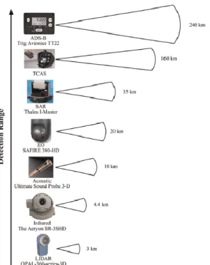
Cooperative SAA methods utilize hardware that communicates between vehicles and ground stations, specifically providing data exchange of locations, trajectories, or other navigationally critical information. The traffic collision avoidance system (TCAS) is currently the method of choice for manned aircraft avoidance (Billingsley, Kochenderfer, & Chryssanthacopoulos, 2011). With a maximum range of 160 𝑘𝑚, TCAS systems create a virtual airspace map for an aircraft, alerting and providing instructions for the pilots if another aircraft intrudes on the airspace (Angelov, 2012).
8
The aviation industry, specifically those interested in SAA, see TCAS as a viable option due to its current and widespread implementation, as well as its functionality for Visual Measurement Conditions (VMC) and Instrument Measurement Conditions (IMC) (Yu & Zhang, 2015). Automatic dependent surveillance – broadcast (ADS-B) is another similar, and proven, cooperative technology that provides participating receivers with aircraft global positioning system (GPS) coordinates, velocity, mission intent, and a specific identification value (Zeitlin & McLaughlin, 2007). While this is not yet a required or fully supported system, ADS-B can supply data exchange 240 𝑘𝑚 to and from ground stations, making it very favorable as a leading SAA technology. Both of these cooperative solutions, however, are limited in a few aspects in regards to use as SAA technology. TCAS is very capable with individual vehicles, but has not been proven to be able to incorporate multiple vehicles. ADS-B has the disadvantage of not working with ground or stationary objects (Yu & Zhang, 2015). The largest drawback of both these cooperative systems as SAA technologies stems from the necessity for all other vehicles to use the same technology to ensure collision trajectories are detected and avoidance maneuvers are made (Angelov, 2012).
Due to cooperative methods needing to be universally implemented, non-cooperative SAA systems have obtained a significant standing for application and research. Non-cooperative SAA methods have the advantage of not requiring communications or broadcasts between vehicles or ground stations. With use of technologies like synthetic aperture radar (SAR), Lidar, acoustic sensors, and electro-optical cameras, UAVs and other vehicles can independently detect and avoid other vehicles, buildings, and ground targets without any interaction with outside communications (Yu & Zhang, 2015).
9
Figure 8: Examples of current SAA technologies and the common range limitations (Yu & Zhang, 2015)
These technologies, having been well established, present advantages and
disadvantages, specifically in the area of physically sensing environments and obstacles surrounding them. SAR, for instance, has the capability to collect location, velocity, and size information about its environment or other vehicles using multiple radar pulses (Yu & Zhang, 2015). In particular, the NASA Jet Propulsion Lab (JPL) has proven the effectiveness of SAR for detection ranges of 16 𝑘𝑚 at a resolution capable of sensing miniature UAVs, and it provides General Atomic’s Predator B with 220° azimuth and 30° elevation field of view (FOV) (Moses, Rutherford, & Valavanis, 2011). While it has a significant advantage of being SAA capable in all weather conditions, one fallback of SAR technology is the limitation of sending and receiving data at the speed of sound, making it difficult for real time implementation. In SAA systems, time becomes a
mission, not a variable, meaning any critical detection and required avoidance maneuvers cannot be fully dependent on a time-consuming method (Yu & Zhang, 2015).
10
Lidar can also provide environment and obstacle location and distance information relative to the UAV, but can also be used to maintain a collection of point cloud data for virtual reconstruction of the environment. This powerful technology has been a tool for Carnegie Mellon University’s Robotics Institute to reduce false positives from other SAA methods, and has the potential to be utilized as a way to “remember” the environment, a concept that can allow for more than fly-through navigation, but also loitering and reconnaissance missions (Geyer, Dey, & Singh, 2009).
Figure 9: Example point cloud scene collected via Lidar measurements (Ryabinin, 2017)
With detection ranges typically between 200 𝑚 and 3 𝑘𝑚 and resolution capabilities of 5 𝑚𝑚, Lidar proves to be an excellent solution for SAA methods. However, a limiting factor for all of this potential is the limited FOV and large amount of data collected. Lidar typically have a relatively limited FOV in either azimuth or elevation, making its
usefulness a function of specific scenarios. Collision avoidance scenarios requiring detection outside of the Lidar FOV places the UAV in an undesirable state. Also, the large amount of data that Lidar can collect poses a problem with data handling and processing to ensure the required computing and electrical power is available to allow for a real-time SAA system (Yu & Zhang, 2015).
11
Acoustic detection systems are not a particularly new technology, but their application for SAA methods is. The passive acoustic non-cooperative collision alert system (PANCAS), developed by Scientific Applications and Research Associates (SARA) Incorporated, is a leading project in the development of acoustic SAA detection systems (Yu & Zhang, 2015).
Figure 10: Relative zones of detection for optical and PANCAS sensing technologies (SARA Inc., 2012)
Using the noise generated by aircraft engines, propellers, and rotors, acoustic microphones can accurately determine intruding vehicle locations and velocities over a large range of frequencies within a sphere of detection, as seen in Figure 10. Because of its recent development, acoustic detection is limited in a number of ways, particularly with respect to its lack of range, poor performance in weather, and non-real time functionality.
Electro-optical (EO) devices use visible light to create an image of the surrounding environment or obstacles in view. The extent of this technology ranges from common, fixed, monocular vision cameras systems, like those used by recreational and professional photographers, to gimballed, panoramic cameras. The popularity of use of EO sensors as a primary or auxiliary SAA technology stems from its advantages of typically being low cost, lightweight, and requiring low power consumption.
12
Figure 11: Aerial, infrared image of wildfires, taken by RQ-4 Global Hawk (US Navy, 2008)
On a large scale, a notable implementation of EO technology for SAA is on Northrop Grumman’s RQ-4 Global Hawk, cooperatively developed by the Air Force Research Laboratory and Defense Research Associates. This system utilizes three optical cameras to produce an effective ±100° azimuth and ±15° elevation FOV (Griffith, Kochenderfer, & Kuchar, 2008). Figure 11 shows an example image, provided by the United States Navy, of Californian wild fires captured by the primary center optical camera. On a smaller scale, optical flow sensors provide a promising and compact method for position determination and tracking at specific altitudes, similar to that in Gageik et. al., where waypoint navigation, position holding, and landing are all autonomously performed on a small quadrotor (Gageik, Strohmeier, & Montenegro, 2013).
EO cameras can, however, be greatly affected by weather conditions and may require an array of devices and sensor suites to be useful (Yu & Zhang, 2015). And while EO devices allow for a range of chosen detection algorithms, the most common of these require a comparatively large amount of data processing for vision-based tracking methods, and in the end still lack a critical piece of information: range. However, many
13
approaches can be implemented in order to overcome this lack of information with EO cameras.
Stereo vision utilizes two monocular EO cameras separated by a small horizontal distance from each other. This distance creates a horizontal offset, known as parallax, between corresponding features within the two images, which can in turn be used to estimate the range to the feature or object of interest. An example of this can be seen in the diagram presented in Figure 12. The capable range of stereo vision cameras relies on a number of factors including disparity distance, focal length of the lenses, and
environment conditions, but their overall capabilities are limited to smaller distance in comparison to other SAA devices (Yu & Zhang, 2015).
Figure 12: Stereovision parallax, demonstrated by the overlapping FOV of camera A and B (Lau, 2012)
A multitude of EO types can be used in this application, including infrared, demonstrated by Chen et al., in which infrared technology bridged the difficulty in detecting and tracking objects in subpar or low quality environments, something that proves difficult when using true-color EO devices (Chen, Cao, Wu, & Huang, January 2014).
14
Homography vision measurements provide an alternative solution that utilizes EO monocular cameras to derive camera translation, rotation, skewing, and scaling. When fixed to a vehicle body reference frame, these transformations can be directly applied to the vehicle, providing useful information for application of vision-based navigation, or position estimation (Zhao, 2012) An important limitation of this approach is that the homography relationship only holds for tracked features that lie in a common 3-D plane.
1.2. Vision-Based Proportional Navigation
Proportional navigation, commonly referred to as constant bearing decreasing range, is a method of utilizing line-of-sight (LOS) angles for the determination of imminent collisions. This technique has been used more commonly in applications of guidance laws for modern guided munitions, known as intercept guidance laws, in which the path to be taken by a primary vehicle is the one in which its distance with an ultimate target approaches zero. Intercept guidance laws that are based on monocular image plane line-of-sight angles use the change in line-line-of-sight to ensure that an intercept occurs. This proportional navigation (Pro-Nav) concept was originally discovered at sea, with ship navigators determining course corrections required for avoidance of other oncoming watercraft. This robust method of collision detection evolved rapidly for application in guided munitions, particularly with advancements in sensor and computing technology. Unlike stereo vision and other monocular vision techniques, at a basic level, vision-based proportional navigation requires much less computational power by utilizing optical flow, providing changes in positions along the image plane and in turn providing the
information necessary to determine the LOS angles. For the objective of achieving intercept trajectories, the rate of change in the LOS angles provides the information
15
necessary to determine if a collision is imminent. By driving the LOS rate to zero and keeping it at zero, an interception or collision will occur, regardless of initial range or heading. Unfortunately, monocular vision-based guidance is unable to provide a critical piece of information that other sensors can: the range to targets. However, this
shortcoming also plays a role in the advantage of Pro-Nav. The computational cost required for vision-based Pro-Nav is noticeably less than the cost required for most other guidance methods that determine and utilize range or distance information. This is also the point where this research seeks to utilize and apply Pro-Nav to its full potential. With an underlying low computational cost, this method can be applied to a very small vehicle with a large number of obstacles, targets, or features, providing a robust solution for incorporating dynamic and static environments into a resultant navigational path.
The investigation into intercept guidance has been present for a long time; however, it was not well defined until 1966, when Cornell University’s Aeronautical Laboratory Inc. work that placed a classification to Pro-Nav. In its basic form, the paper published was related to missile/seeker interception with a target, using satellites as an example. Characteristics and limitations of Pro-Nav were presented and included optimal values for the Pro-Nav constant, 𝑁𝐻, best performance with and without continuous modulation of thrust, and inclusion of dead space with small LOS rate values (Murtaugh & Criel, 1966). Since then, more advanced methods of Pro-Nav intercept have been examined, notably in work by Cornell University and the United States Army. In this work, the attitude angle at waypoint interception for a guided reentry vehicle is controlled using a time-varying gain, rather than the constant gains defined by Murtaugh and Criel (Kim & Grider, 1973). With the implementation of a linear quadratic controller, Kim and Grider’s
16
work has been distinguished as pioneering, and a notable stepping stone upon which others have expanded, including work by Kim, Lee, and Han, which was a particularly noteworthy implementation of Pro-Nav in which a bias was used to ensure a zero miss distance for a nonlinear analytical model of an intercepting vehicle (Kim, Lee, & Han, 1998).
In relation to this thesis, vision-based Pro-Nav using EO pixel information has been investigated in the context of developing intercept guidance laws for micro aerial vehicles (MAVs) (Beard, Curtis, Eilders, Evers, & and Cloutier, 2007). In this paper, Beard et al. derive Pro-Nav guidance intercept commands based solely on pixel information. This contrasts with the work by Han, Bang, and Yoo, which manipulates Murtaugh & Criel’s original Pro-Nav definiton to fullfill avoidance criteria. Their proposed method utilizes a predicted zone of influence, which the primary vehicle must manuever away from (Han, Bang, & Yoo, 2009). Sharma et al. and Trinh et al. also implement modified methods of Han, Bang, and Yoo’s work in applications to path planning and planar navigation. While these works do not completely describe the amount of research and development that has been put towards Pro-Nav guidance and navigation, they are among the most notable. However, the one contrasting aspect that these works all have in common is the assumption of known range to targets or obstacle. These distances play a part in
determining the time-to-target and using that information to develop successful intercept or avoidance commands.
This thesis extends previous work in regards to using Pro-Nav guidance law for intercept and avoidance guidance to a set of guidance laws that will enable a UAV to avoid multiple dynamic and static obstacles. These algorithms are studied within a
17
simulation environment, utilizing a six degree of freedom (DoF) dynamic model, without the use of target and obstacle range. The results of these simulations are quantified and analyzed for each set of guidance laws in order to determine characteristics and traits, allowing for successive variations and improvements in methodology and algorithmic process. The performance of these algorithms are quantified in terms of the minimization of collision probability.
The path of this thesis takes a developmental approach towards a final Pro-Nav avoidance law capable of avoiding dynamic and static obstacles using Pro-Nav concepts, without the use of range information. The approach systematically characterizes guidance law traits that contribute both positively and negatively, such that these can be taken into consideration for the next iteration of avoidance law development. The final form of the Pro-Nav guidance law is then implemented into a “camera-in-the-loop” simulation environment, where point-of-view images are captured in a realistic virtual environment, processed through an image feature detection algorithm, and applied to the design and implementation of Pro-Nav guidance laws to update the six DoF UAV model’s dynamic response.
18
2. UAV AND CAMERA MODELING
This thesis presents the development of collision-avoidance guidance laws based on monocular vision and the principle of proportion navigation. The approach uses two different mathematical UAV simulation models: one during the beginning and middle stages of guidance law design and testing, and one for final realization and finalization of the chosen law. Both models utilize the 12 aircraft equations of motion to allow for nonlinear, six degree of freedom (DoF) UAV dynamics to be computed in a simulation environment. A waypoint guidance law provides an underlying goal for the UAV to achieve during all simulations (with the exception of intercepting guidance cases). Altitude and velocity are maintained during maneuvering using PID controllers that maintain pitch and velocity by changing elevator and thrust values. The primary method of lateral maneuvering is uses a bank-to-turn heading controller, shown in Figure 13, which converts a commanded change of a selected heading parameter to a commanded bank angle, 𝜙𝑐𝑜𝑚, with the proportional gain 𝐾𝜙𝑐𝑜𝑚. The controller then converts the commanded change in bank angle to an aileron command, 𝛿𝑎𝑐𝑜𝑚, with a PID controller. It is important to note that Δ𝜓𝑐𝑜𝑚 is a resultant change in heading derived from the implementation of a Pro-Nav based guidance law.
19
While the modeling and control are similar for both UAVs, the initial conditions and geometric parameters differ greatly, which are discussed further below.
2.1. Medium-Scale, Propeller UAV Model
The initial aircraft model used for development of the Pro-Nav guidance laws represents a medium scale, propeller driven UAV. Some important aircraft geometric properties and flight conditions are shown in Table 1.
Table 1: Medium scale UAV geometric and flight parameters
Parameter Value Units
bw 33.4 𝑓𝑡
Aw 6.06
Vo 176.4 𝑓𝑡/𝑠
ho 1000 𝑓𝑡
In Table 1, 𝑏𝑤 is the UAV wing span from tip to tip and 𝐴𝑤 is the wing aspect ratio, which relates the wing span to the wing surface area 𝑆𝑤 using the equation 𝐴𝑤 =𝑏𝑤
2 𝑆𝑤.
𝑉𝑜 and ℎ𝑜 are the UAV trim velocity and altitude, respectively. This model was provided
by students in the Embry-Riddle Flight Dynamics and Control Research Laboratory (FDCRL) that includes PID tracking controllers for velocity, altitude and roll angle. Control tests were conducted initially using waypoint navigation to ensure the validity of the controller gains.
2.2. Small-Scale, RC Propeller UAV Model
The Condor Skywalker 1880 was used as a representative model for a small-scale, RC propeller driven UAV, and modified accordingly to achieve greater lateral dynamic stability and response. The geometric properties and trim flight conditions are shown in Table 2 for comparison with the medium-scale UAV model.
20
Table 2: Small-scale UAV geometric and flight parameters
Parameter Value Units
bw 5.43 𝑓𝑡
Aw 5.06
Vo 45.3 𝑓𝑡/𝑠
ho 23.0 𝑓𝑡
This aircraft model was also provided by FDCRL students; however, the control laws were designed specifically for this research. Like the medium-scale UAV model, the control laws utilize PID controllers for altitude, velocity, and bank control, designed via the Ziegler-Nichols PID tuning method (Nelson, 1998).
2.3. Camera Model
A projective, pinhole camera model is the projection of three-dimensional geometry of the scene via a pinhole camera model, and can be represented by using three primary coordinate systems: the camera frame 𝐶 (in some instances also denoted by 𝑀), body-fixed frame 𝐵, and navigational frame 𝐸. The use of a camera model in this thesis can be broken up into two primary methods. The first model, implemented for point-mass simulations, uses given point-mass locations in the inertial reference frame, also known as the north-east-down (𝑁𝐸𝐷) frame. The reference frame is a local coordinate system in which 𝑥 and 𝑦 are aligned with the magnetic north and east poles of earth, with 𝑧 oriented positively in the downwards direction. This camera modeling method computes the vector projection normalized about a focal-axis. For this case, the camera-fixed focal-axis is aligned with the 𝑁𝐸𝐷 𝑥-axis, resulting in the following normalized vector:
21 { 𝑥 𝑦 𝑧}𝑝/𝑐 𝐸 = 𝑟𝑝𝐸 − 𝑟𝑐𝐸 → { 1 (𝑦𝑝/𝑐 𝐸 𝑥𝑝/𝑐𝐸 ) (𝑧𝑝/𝑐 𝐸 𝑥𝑝/𝑐𝐸 ) } 𝐸 (1)
where 𝑟̲𝑝𝐸 and 𝑟̲𝑐𝐸denote the inertial position of the target feature point and the UAV center of mass, respectively. It is important for the point-masses (or feature points) to be expressed with respect to the inertial frame when implementing Pro-Nav guidance laws. This means a few steps are not required when utilizing this camera model method, since the point locations are already provided in the inertial reference frame. However, multiple additional processing steps are required when using a real camera/EO device or a virtual reality environment.
In real-world or virtual scenarios and simulation, the latter of which will be presented later in this thesis, the locations of feature points are provided in the two- dimensional camera frame, also known as the pixel frame. These pixel coordinates are converted to the inertial reference frame via the use of a camera calibration matrix, a camera-to-body frame rotation matrix, and a body-to-inertial frame rotation matrix, commonly known as the direction cosine matrix (DCM) with respect to the aircraft. This calculation can be represented as:
𝑥𝑝/𝑐𝐸 = 𝑅
𝑐𝐸𝐾𝑥𝑝/𝑐𝑐 (2)
In Equation (2), 𝑥𝑐 and 𝑥𝐸 are the feature point relative to the camera coordinates with respect to the camera-pixel frame and the inertial frame, respectively. 𝐾 is the intrinsic calibration matrix that transforms the pixel coordinates into real-world camera coordinates. These real-world coordinates are values with physical units rather than pixel
22
dimensions. A physical representation of this conversion can be seen in Figure 14.
𝐾 = [
𝛼𝑥 𝛾 𝑢𝑜 0 𝛼𝑦 𝑣𝑜
0 0 1
] (3)
Equation (3) shows the specific form of the intrinsic calibration matrix, in which 𝛼𝑥 and 𝛼𝑦 represent the focal length in terms of image pixels, and 𝛾 provides a coefficient to compensate for any skew angle between the 𝑥 and 𝑦 axis of the focal plane. 𝑢𝑜 and 𝑣𝑜 are the principle point, which is the center of the image with respect to the pixel coordinates.
Figure 14: Visual representation of image and focal plane related by intrinsic matrix (OpenMVG, 2013)
The calibrated coordinates are then transformed by the previously mentioned DCM and camera-to-body rotation, represented by 𝑅𝑐𝐸, which will be defined further in the next section of this thesis.
2.4. Simulation Environment
MATLAB/Simulink is the primary simulation environment for the work presented in this thesis. MATLAB coding is used alongside Simulink block diagrams to simulate the guidance and navigation of a six degree-of-freedom aircraft model. The diagram in Figure 15 shows the point-mass simulation process, in which the aircraft model sends its position and orientation information to a vision measurement block so that the vision
23
based measurements of the obstacles relative to the UAV can be derived. The guidance commands produced by this block then send information for the tracking PID controllers to produce a commanded control input that the UAV model can interpret.
Figure 15: Diagram of Simulink block configuration for point mass simulations
The aerodynamics of the UAV model are shown in Figure 16, where a component buildup method using aerodynamic coefficients is implemented to determine the resultant aerodynamic forces and moments. Although there is more complexity to the UAV model, the application of these aerodynamic coefficients contributes largely to the dynamics exhibited by the aircraft. Each coefficient has a subset of contributing derivatives, such as from the wing, elevator, or aileron.
24
Figure 16: Aerodynamic component buildup for six DoF model
Figure 17 shows a simulation diagram similar to that seen in Figure 15, but applicable to the simulation supporting virtual environment simulations. In this diagram,
communication must be made to an application outside of the simulation environment. Information must then be received from the application before the simulation can continue. This information is then used to produce a guidance command and in turn, control the aircraft. This simulation configuration will be discussed further in depth in Chapter 8.
25 3. PRO-NAV INTERCEPT LAW
The Pro-Nav intercept laws provide a mathematically derived heading and flight angle command to the UAV, which in turn initiates aileron and elevator control commands to avoid the obstacle. The commanded heading and flight path angles are determined using the information provided in the monocular image plane, specifically the horizontal and vertical location of the target(s) relative to the center of the image plane.
Figure 18: LOS Angles with respect to the Image Plane.
On the left of Figure 18, the three-dimensional camera frame, with respect to the image plane, shows the horizontal and vertical line of sight angles, 𝜒 and 𝛾, derived from the projected target locations, 𝑥𝑚 and 𝑦𝑚 on the image plane in the camera reference frame. 𝑟̂𝑝/𝑐𝐸 = {𝑥̂𝑦̂ 𝑧̂ } 𝐸 = 𝑅𝑐𝐸𝐾𝑟̂𝑝/𝑐𝑐 = 𝑅𝑐𝐸𝐾 { 𝑥𝑚 𝑦𝑚 1 } 𝐶 (4)
26 𝑅𝑐𝐸 = 𝑅𝐵𝐸𝑅𝑐𝐵= (𝐷𝐶𝑀)𝑇[ 0 −1 0 0 0 1 1 0 0 ] 𝐹𝑖𝑥𝑒𝑑 𝐶𝑎𝑚𝑒𝑟𝑎 (5) 𝑅𝐵𝐸 = (𝐷𝐶𝑀)𝑇 = [
cos 𝜃 cos 𝜓 sin 𝜙 sin 𝜃 cos 𝜓 − cos 𝜙 sin 𝜓 cos 𝜙 sin 𝜃 cos 𝜓 + sin 𝜙 sin 𝜓 cos 𝜃 sin 𝜓 sin 𝜙 sin 𝜃 sin 𝜓 + cos 𝜙 cos 𝜓 cos 𝜙 sin 𝜃 sin 𝜓 − sin 𝜙 cos 𝜓
− sin 𝜃 sin 𝜙 sin 𝜃 cos 𝜙 cos 𝜃 ]
(6)
This derivation, shown in Equations (4) through (6), is obtained through the rotation matrix RcE and assumes the camera is fixed relative to the UAV. For the cases studied in
this thesis, the camera is assumed to be pointed in the body-x direction; therefore, the RCB defined in Equation (5) simply reorders the camera axes to coincide with the body-fixed axes. The resulting LOS angles, along with their respective LOS angular rates, can then be derived as follows: 𝜒𝐿𝑂𝑆 = 𝑡𝑎𝑛−1(𝑦̂𝑝/𝑐𝐸 𝑥̂𝑝/𝑐𝐸 ) → 𝜒̇𝐿𝑂𝑆(𝑡𝑘) = 𝜒𝐿𝑂𝑆(𝑡𝑘) − 𝜒𝐿𝑂𝑆(𝑡𝑘−1) 𝛥𝑡 (7) 𝛾𝐿𝑂𝑆 = 𝑠𝑖𝑛−1 ( 𝑧̂𝑝/𝑐𝐸 √𝑥̂𝑝/𝑐𝐸 2+ 𝑦̂ 𝑝/𝑐𝐸 2)) → 𝛾̇𝐿𝑂𝑆(𝑡𝑘) = 𝛾𝐿𝑂𝑆(𝑡𝑘) − 𝛾𝐿𝑂𝑆(𝑡𝑘−1) 𝛥𝑡 (8)
Equations (7) and (8) form the basis for the laws implemented in an intercept based simulation, in which a medium-scale UAV seeks to intercept and “collide” with a target moving at a constant velocity and heading. For an intercept to be made, the simulated UAV uses Equation (9) and (10) to initiate commanded heading and flight path angles. These longitudinal and lateral commands can vary, based on the method of
27
𝜓̇𝑐𝑜𝑚= 𝑁𝐻𝜒̇𝐿𝑂𝑆 → {Δ𝜓Δ𝜙𝑐𝑜𝑚 = 𝑁𝐻𝜒̇𝐿𝑂𝑆Δ𝑡𝑇
𝑐𝑜𝑚 = 𝑘𝜙Δψcom (9)
𝛾̇𝑐𝑜𝑚 = 𝑁𝑣𝛾̇𝐿𝑂𝑆 → Δ𝛾𝑐𝑜𝑚 = 𝑁𝑣𝛾̇𝐿𝑂𝑆Δ𝑡𝑇 (10) Equations (9) and (10) are the proportional guidance commands that use proportional gains NH and NV to provide a commanded rate of change of yaw and vertical flight path angles. These constant are the proportional navigation constants that enable the concept of Pro-Nav to be successful. The optimal values have been previously been determined to be optimized at three (Murtaugh & Criel, 1966). Calculating the rate of change in LOS angles using finite differences allows the flight commands to be referenced to where the target will be in the next iteration. Results of the implementation of this intercept
guidance controller can be seen in Figure 19 - Figure 21, in which a few representative examples of the numerous scenarios simulated are presented with an active intercept controller for the UAV and different headings for the target.
Figure 19: Example 1 - UAV Intercept path (units in feet).
28
of −90°, starting from one mile north and one mile east of the UAV. Both the UAV and target obstacle are traveling at the same initial velocity, which is the case for the rest of the scenarios as well. The similar velocities for the scenario in Figure 19 would mean the optimal UAV intercept path would be to continue on a constant north heading. The deviation seen in the path shows the intercept guidance law at work, generating control inputs based on the LOS angular rates rather than relative distances and velocities, which are assumed to be unknown.
Figure 20: Example 2 - UAV Intercept path (units in feet).
Figure 20 shows another engagement using the intercept controller, similar to the one presented in Figure 19, except that the target starting location is one mile north and half a mile east relative to the UAV. The controller’s effectiveness is seen almost immediately by the UAV’s deviation westward to intercept the target.
29
Figure 21: Example 3 - UAV Intercept path (units in feet).
The scenario shown in Figure 21 differs from the previous two in that the obstacle has an initial starting point a half mile north and one mile west of the UAV, with a heading of 26.6°. This scenario aids in verifying the functionality of the controller by having a target traveling from the opposite side as the previous cases. This shows that the sign of the calculated 𝜒̇ is accounted for and interpreted correctly, regardless of which direction the represented target is moving across the image plane.
30
4. PRO-NAV AVOIDANCE LAW – THRESHOLDING APPROACH
Extending the intercept guidance law to avoidance based guidance laws requires a modified set of control laws. Specifically, the modified guidance laws must first
determine if a collision avoidance maneuver is required and then compute the magnitude and direction of the avoidance maneuver that should be made. These two criteria are accounted for by using a threshold activation controller and a piecewise directional controller.
The threshold activation controller compares the absolute value of the LOS angular rates with a selected threshold value. A zero LOS angular rate implies an imminent collision between the UAV and target, so that setting a threshold value to zero would only ensure any avoidance distance, no matter how small, would be acceptable.
Therefore, a small threshold value is implemented to command an avoidance maneuver for LOS angular rates close to zero. When considering the size of a medium size UAV, an avoidance larger than 20 𝑓𝑡could be considered an acceptable distance, although this would depend on the size and speed of the other vehicle. The distance to the target is assumed to be unknown, but the threshold parameter determines the degree of resulting avoidance distance and sensitivity of the avoidance law. This is an area that was first investigated, with the results summarized in Table 3 - Table 5.
In regards to commercial flight, when an incident occurs in which an avoidance maneuver is required, the FAA has regulated lateral maneuvering to be the primary course of action. The direction of this lateral maneuver, however, is not defined. The avoidance law implemented in this thesis uses the following logic, in which 𝜓̇𝑐𝑜𝑚 is selected to be a constant value:
31
ψcom= { ψ̇com∆𝑡𝑐, χ̇ ≤ 0 −ψ̇com∆tc, χ̇ > 0
This piecewise directional controller uses the logic of traveling behind the intercepting target, relative to its velocity and heading. Therefore, a negative LOS angular rate results in a positive commanded heading, while a positive LOS angular rate produces a negative commanded heading. Zero was included in the first definition of the piecewise function to favor deviating behind the collision threat. Any zero LOS rate requires some form of action to be taken, and without a direction of the intercepting obstacle, any reaction in a direction provides a better choice than not maneuvering at all.
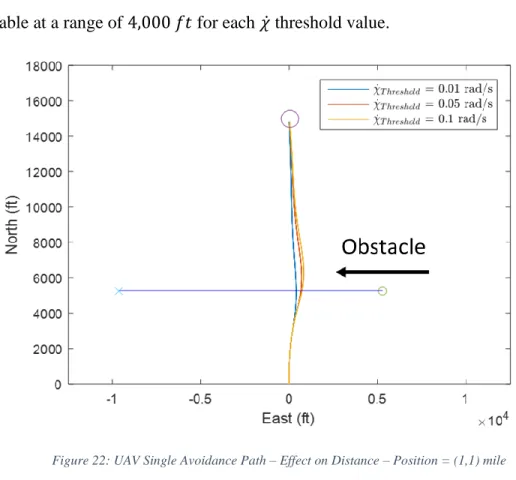
Several dynamic avoidance scenarios were used to demonstrate and further develop the avoidance controller. These scenarios are similar to those used for the intercept simulations. The initial conditions for the dynamic obstacles are varied in terms of obstacle heading, starting location, and velocity. A major difference between these simulations and the intercept simulations is that these initial conditions are modified to ensure an imminent collision if an avoidance maneuver is not made. Figure 22 - Figure 24 show the first configuration set of three simulations. In this set, the obstacle velocity and heading are held constant at 176 𝑓𝑡/𝑠 and −90°, respectively, while the starting location of the obstacle is varied proportionally to ensure that an imminent collision along the north axis will occur if no avoidance maneuver is performed. By varying the range alone for this set of simulations, insight can be gained on the effectiveness of range on avoidance distance over a variety of threshold 𝜒̇ values. Figure 22 shows the first of the three simulations varying range and holding all other variables constant. For this simulation, the initial position of the obstacle is one mile north and one mile east of the
32
UAV. The avoidance controller produces a deviation in the UAV path that becomes noticeable at a range of 4,000 𝑓𝑡 for each 𝜒̇ threshold value.
Figure 22: UAV Single Avoidance Path – Effect on Distance – Position = (1,1) mile
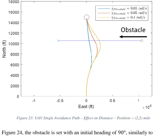
Figure 23 presents a similar scenario for investigating the effect of distance on avoidance distance using the Pro-Nav avoidance controller. The obstacle location, however, is set to two miles north and two miles east, ensuring that an intercept will occur two miles in front of the UAV along the north axis with no avoidance controller active. The simulations were computed for threshold values of 0.005, 0.01, and 0.02 𝑟𝑎𝑑/𝑠 and show avoidance maneuvers implemented.
33
Figure 23: UAV Single Avoidance Path – Effect on Distance – Position = (2,2) mile
In Figure 24, the obstacle is set with an initial heading of 90°, similarly to the simulations in Figure 22 and Figure 23, but with a starting position of half a mile north and half a mile east. This is the third simulation in the set of three to investigate the effect of distance on the avoidance controller’s capability of ensuring an imminent collision is prevented. This path does not lead to a collision without active avoidance, but does not follow the trend of the previous scenarios, initiating an avoidance maneuver at around 2,000𝑓𝑡 for each simulation of 𝜒̇ threshold values of 0.005, 0.01, and 0.02 𝑟𝑎𝑑/𝑠.
34
Figure 24:UAV Single Avoidance Path – Effect on Distance – Position = (0.5,0.5) mile
Table 3 summarizes the results for the effect of obstacle range on avoidance distance from the obstacle. One noticeable trend for all avoidance thresholds simulated is an increase in avoidance distance with an increase in obstacle starting position and intercept distance. However, the increase in avoidance distance with the increase in 𝜒̇ threshold is not significant at shorter obstacle distances but does become effective at larger distances. Overall, it can be said that the guidance controller is more effective at avoiding obstacles further away than obstacles that are closer, with the value of 𝜒̇ threshold being more significant at further distances.
35
Table 3: UAV Single Avoidance, Effect of Position, V=176 ft/s
𝝌̇𝑻𝒉𝒓𝒆𝒔𝒉𝒐𝒍𝒅 (rad/sec)
0.01 0.05 0.1
Position (ft, ft) Miss Distance (Guidance On) Miss Distance (No Guidance) (2,640, 2,640) 78 ft 90 ft 91 ft 1.2 ft (5,280, 5,280) 289 ft 457 ft 487 ft 1.2 ft (10,560, 10,560) 482 ft 1,661 ft 2,175 ft 1.6 ft
The second set of simulations, the results of which are shown in Table 4, explore the effect of velocity on the UAV’s avoidance distance from the obstacle. For the simulations, the obstacle is set with an initial heading of −90° (due west), and has a varying velocity and initial east position. The position is increased proportionally with the speed to ensure a collision occurs along the north axis if an avoidance maneuver is not performed. An overarching interpretation of the results in Table 4 is that higher obstacle velocity, relative to the UAV velocity, leads to larger avoidance distances between the obstacle and UAV.
Table 4: Single Avoidance Effect of Velocity, V=88, 176, 264 ft/s
𝝌̇𝑻𝒉𝒓𝒆𝒔𝒉𝒐𝒍𝒅 (rad/sec)
0.01 0.05 0.1
Position (ft, ft) Miss Distance (Guidance On) Miss Distance (No Guidance) (5,280, 2,640) 286 ft 530 ft 587 ft 1.2 ft (5,280, 5,280) 289 ft 457 ft 487 ft 1.2 ft (5,280, 10,560) 282 ft 395ft 411ft 1.3 ft
The scenario results presented in Table 5 are based on obstacle engagements where the UAV is not initially placed on a collision path. This means that the miss distances between the obstacle and UAV with no active avoidance in Table 5 are already sufficient, such that any added control input can be considered unnecessary, unlike the scenarios in Table 3, which required avoidance maneuvers.
36
Table 5: Single Avoidance No Intercept, V=88, 176, 264 ft/s
𝝌̇𝑻𝒉𝒓𝒆𝒔𝒉𝒐𝒍𝒅 (rad/sec)
0.01 0.05 0.1
Position (ft, ft) Miss Distance (Guidance On) Miss Distance (No Guidance) (2,640, 2,640) 1,867 ft 1,994 ft 2,075 ft 1,870 ft (5,280, 5,280) 2,368 ft 2,565 ft 2,562 ft 2,361 ft (10,560, 10,560) 1,469 ft 1,605 ft 1,654 ft 1,464 ft
The simulation sets presented in Table 3 - Table 5 show that the application of the Pro-Nav guidance law was successful in providing acceptable avoidance distance between the UAV and obstacles when initially set for intercepting paths. While some unnecessary maneuvering does occur, specifically when no collision is present, the amount of overcompensation is not considered to be excessive.
37
5. PRO-NAV AVOIDANCE LAWS – MOST IMMINENT THREAT
With a proven method for single obstacle avoidance using LOS rate thresholds, the next step was to apply this controller to a more complicated scenario. Introducing a second intercepting target adds an element of risk when executing an avoidance
maneuver. Successful avoidance of one moving obstacle may lead to an intercepting path with the other obstacle. In this section, the avoidance guidance laws are applied in
scenarios involving multiple collision threats.
To investigate these scenarios, the simulation environment first introduces two constant velocity obstacles at independent starting locations and headings. Due to the second obstacle being present in the simulation, the projection method for simulating a camera view exhibits two feature points, meaning the implemented guidance law has to be updated to process LOS angular rates for both obstacles. The modified law’s primary method of deciding on an avoidance maneuver is prioritization of the smallest LOS rate value at time 𝑡𝑘 between both targets. This most imminent threat strategy entails
maneuvering to avoid the target with the smallest LOS rate, which is indicative of the most serious collision threat, while not reacting to the other obstacles in the scene. This strategy is the applied to a scene with multiple static obstacles.
5.1. Dynamic Avoidance
Several multiple engagement scenarios were simulated in which constant velocity obstacles were placed at starting positions and headings that would ensure an intercept is inevitable with at least one of them by the UAV. In some cases, one obstacle is
positioned to intercept or have a near-intercept situation with the UAV as it attempts to avoid the other obstacle. For each scenario, the controller was set to actively avoid each
38
target individually for two individual simulations, followed by a third simulation with multi-avoidance active.
In Figure 25, both obstacles have an initial heading of −90° and starting positions such that they result in a collision with the UAV along the North axis. On the left side of the figure, a single avoidance simulation was performed in order to determine the miss distance between both obstacles and the UAV while attempting to avoid the closer of the obstacles, Obstacle 1.
Figure 25: UAV Individual Avoidance Paths (ft) - Obstacle 1 and 2 North Intercept - 𝜒̇ = .01𝑑𝑒𝑔𝑠
Table 6 shows the obstacle offsets and miss distances from the simulations in Figure 25. For the first simulation, in which Obstacle 1 is being avoided without regards to Obstacle 2, there is an avoidance distance of 457 𝑓𝑡 between Obstacle 1 and the UAV. Obstacle 2 is avoided by 237 𝑓𝑡, but it is important to note that this avoidance is only inherited by the intent to avoid Obstacle 1. For the second simulation, on the right of Figure 25, active avoidance of Obstacle 2 only resulted in an avoidance distance of 506 𝑓𝑡 for Obstacle 2 and 1,661 𝑓𝑡 for Obstacle 1, noting again the miss distance between Obstacle 1 and the UAV is inherited.
39
Table 6: UAV Individual Avoidance Data - Obstacle 1 and 2 North Intercept
Obstacle 1 Miss Distance (ft) Obstacle 2 Miss Distance (ft) Obstacle 1 Avoidance 457 237 Obstacle 2 Avoidance 506 1,661
The simulations for which the multi-avoidance controller was enabled can be seen in Figure 26. These simulations are represented by the UAV paths for a chosen set of 𝜒̇ threshold values, including 0.01, 0.05, and 0.1𝑑𝑒𝑔𝑠 . The resulting path resembles that of a superposition of the simulations in Figure 25, with an increase in path deviation because of the increased 𝜒̇ threshold.
Figure 26: UAV Multi-Avoidance Paths (ft) - Obstacle 1 and 2 North Intercept
Justification for the increasing path deviations in Figure 26 can be seen in Table 7, where the avoidance distance for both Obstacles 1 and 2 are larger the 400 𝑓𝑡. This avoidance distance differs slightly from the original 𝜒̇ threshold avoidance controller for
40
single obstacle avoidance; however, the results support the previous trend of increasing 𝜒̇ threshold values from the single avoidance cases.
Table 7: UAV Multi-Avoidance Data - Obstacle 1 and 2 North Intercept
𝝌̇ Threshold (rad/s) Obstacle 1 Miss Distance (ft) Obstacle 2 Miss Distance (ft) 0.01 502 482 0.05 506 1661 0.10 506 2175
For the single obstacle avoidance controller, the sensitivity of the controller was investigated with a scenario in which the obstacle was not set on an intercepting path. Figure 27 shows the avoidance path for the first of two similar multi-avoidance scenarios. Obstacle 2 is set to not intercept the UAV along the north axis, but instead along the path taken to avoid Obstacle 1 only. By doing this, the avoidance sensitivity can be assessed along with the reactiveness of the controller. Because avoiding Obstacle 1 will place Obstacle 2 on a collision course, it is critical to see what kind of avoidance maneuver will be taken, if at all, and whether it is enough to avoid both obstacles with enough distance without overcompensating.
41
In Table 8, the 457 𝑓𝑡 miss distance of Obstacle 1 and the 1.3 𝑓𝑡 miss distance of Obstacle 2 correlates to the simulation on the left in Figure 27, where the avoidance controller is active for Obstacle 1. The small avoidance distances between Obstacle 2 and the UAV can be interpreted as an intercept and the focus of this simulation. On the right of Figure 27, the avoidance of Obstacle 2 leads to a similar avoidance of Obstacle 1 and 2, the distance being 443 𝑓𝑡 and 759 𝑓𝑡, respectively. The avoidance distance between Obstacle 1 and the UAV is only an inherited aspect, due to the avoidance controller actively avoiding only Obstacle 2.
Table 8: UAV Individual Avoidance Data - Obstacle 2 Offset Intercept
Obstacle 1 Miss Distance (ft) Obstacle 2 Miss Distance (ft) Obstacle 1 Avoidance 457 1.3 Obstacle 2 Avoidance 443 759
Figure 28 shows the multi-avoidance path of the UAV for a North intercept of Object 1, with a starting position East of the UAV, and an East offset intercept of Object 2, initially starting East as well. The paths deviate similarly to those in Figure 26, having a larger deviation with a larger 𝜒̇ threshold value, and resembling the superposition of the individual avoidance maneuvers in Figure 27.
42
Figure 28: UAV Multi-Avoidance Paths (ft) - Obstacle 2 Offset Intercept
The miss distances shown in Table 9 correspond to the avoidance paths shown in Figure 28. An increase in 𝜒̇ threshold, like previous simulations, increases the avoidance distance, but only slightly with regards to Obstacle 2, with a maximum closest distance of 515 𝑓𝑡 between the Obstacle 2 and UAV for a 𝜒̇ threshold of 0.05𝑑𝑒𝑔𝑠 .
Table 9: UAV Multi-Avoidance Data - Obstacle 2 Offset Intercept
𝝌̇ Threshold (rad/s) Obstacle 1 Miss Distance (ft) Obstacle 2 Miss Distance (ft) 0.01 6.7 454 0.05 6.7 515 0.10 6.7 515
Figure 29 shows the multi-avoidance path of the UAV for a north intercept of Object 2, with a starting position East of the UAV, and an East offset intercept of Object 1, initially starting East as well, such that no intercept is to occur if no maneuver is made. The path in avoidance of Obstacle 1 deviates opposite to that seen in Figure 27, resulting
43
in an avoidance maneuver left of Obstacle 1. This is due to the obstacle being offset east, leading the avoidance law to travel the safest path, being in front of the obstacle.
Figure 29: UAV Individual-Avoidance Paths (ft) - Obstacle 1 Offset Intercept
Table 10 shows an 830 𝑓𝑡 miss distance of Obstacle 1 and the 63 𝑓𝑡 miss distance of Obstacle 2, correlating to the simulation on the left in Figure 29, where the avoidance controller is active for Obstacle 1. The avoidance distances between Obstacle 2 and the UAV is large enough to be interpreted as a safe engagement. On the right of Figure 29, the avoidance of Obstacle 2 leads to an avoidance of Obstacle 1 that is less than Obstacle 2, the distances being 1.8 𝑓𝑡 and 1,661 𝑓𝑡, respectively. This avoidance distance between Obstacle 1 and the UAV can clearly be defined as a collision due to the inherited aspect of the avoidance controller actively avoiding Obstacle 2 only.
Table 10: UAV Individual Avoidance Data - Obstacle 1 Offset Intercept
Obstacle 1 Miss Distance (ft) Obstacle 2 Miss Distance (ft) Obstacle 1 Avoidance 830 63 Obstacle 2 Avoidance 1.8 1,661
44
The scenarios in Figure 29 are again presented in simulations for which the multi-avoidance controller was enabled, seen in Figure 30. These simulations are represented by the UAV paths for a chosen set of 𝜒̇ threshold values, including 0.01, 0.05, and 0.1𝑑𝑒𝑔𝑠 . The resulting path resembles that seen in the right-hand side of Figure 29, where Obstacle 2 was the only obstacle actively avoided. The same trend previously seen in multi-avoidance simulations is present in this case as well, with an increase in path deviation due to an increased 𝜒̇ threshold.
Figure 30: UAV Multi-Avoidance Paths (ft) - Obstacle 1 Offset Intercept
The miss distances shown in Table 11 relate to the avoidance paths shown in Figure 30. An increase in 𝜒̇ threshold, like previous simulations, increases the avoidance distance, but only with regards to Obstacle 2, with a maximum closest distance of 1,481 𝑓𝑡 between Obstacle 2 and the UAV for a 𝜒̇ threshold of 0.05𝑑𝑒𝑔𝑠 . However, the avoidance of Obstacle 1 is not only small, but decreases as the avoidance threshold