A Consistent Pricing Model for Index Options and Volatility Derivatives

(1)

WORKING PAPER F-2009-05

Rama Cont & Thomas Kokholm

A Consistent Pricing Model for Index Options and

Volatility Derivatives

Finance

(2)

A Consistent Pricing Model for

Index Options and Volatility Derivatives

∗

Rama Cont

Center for Financial Engineering Columbia University, New York

[email protected]

Thomas Kokholm†

Aarhus School of Business Aarhus University

[email protected]

September 17, 2009

Abstract

We propose and study a flexible modeling framework for the joint dynamics of an index and a set of forward variance swap rates writ-ten on this index, allowing options on forward variance swaps and options on the underlying index to be priced consistently. Our model reproduces various empirically observed properties of variance swap dynamics and allows for jumps in volatility and returns.

An affine specification using L´evy processes as building blocks leads to analytically tractable pricing formulas for options on variance swaps as well as efficient numerical methods for pricing of European op-tions on the underlying asset. The model has the convenient fea-ture of decoupling the vanilla skews from spot/volatility correlations and allowing for different conditional correlations in large and small spot/volatility moves.

We show that our model can simultaneously fit prices of European options on S&P 500 across strikes and maturities as well as options on the VIX volatility index. The calibration of the model is done in two steps, first by matching VIX option prices and then by matching prices of options on the underlying.

∗_{Presented at the 19th Annual Derivatives Securities and Risk Management Conference}

2009 and the Nordic Finance Network Workshop 2009.

†_{A first draft of this paper was completed while Thomas Kokholm held a visiting}

scholar position at the Graduate School of Business (GSB), Columbia University, and he wishes to thank Bjørn Jørgensen and the accounting division at GSB for placing their facilities at his disposal. Moreover, thanks to Bjarne Astrup, Peter Løchte Jørgensen and Elisa Nicolato for comments.

(3)

Introduction

Volatility indices –such as the VIX index– and derivatives written on such indices have gained popularity in markets as tools for hedging volatility risk and as market-based indicators of volatility. Variance swap contracts [19] are increasingly used by market operators to take a pure exposure to volatility or hedge the volatility exposure of options portfolios.

The existence of a liquid market for volatility derivatives such as VIX options, VIX futures and a well developed over-the-counter market for op-tions on variance swaps, and the use of variance swaps and volatility index futures as hedging instruments for other derivatives have led to the need for a pricing framework in which volatility derivatives and derivatives on the underlying asset can be priced in a consistent manner. In order to yield derivative prices in line with their hedging costs, such models should be based on a realistic representation of the joint dynamics of the underlying asset and variance swaps written on this, while also be able to match the observed prices of the liquid derivatives –futures, calls, puts and variance swaps– used as hedging instruments.

In principle, any continuous-time model with stochastic volatility and/or jumps implies some joint dynamics for variance swaps and the underlying asset price. Broadie and Jain [8] studied the valuation of volatility deriva-tives in the Heston model; Carr et al. [11] study the pricing of volatility derivatives in models based on L´evy processes. However, in many com-monly used models the dynamics implied for variance swaps is unrealistic [10, 5]: for example, exponential L´evy models imply a constant variance swap term structure while one-factor stochastic volatility models predict perfect correlation among movements in variance swaps at all maturities.

Also, as pointed out by Bergomi [5, 7], the joint dynamics of forward volatilities and the underlying asset is neither explicit nor tractable in most commonly used models, which makes parameter selection/calibration diffi-cult and does not enable the user to choose a parameter to take a view on forward volatility. As a result, classical models such as the Heston model or (time changed) exponential-L´evy models are unable to match empirical properties of variance swaps and VIX options [5, 7, 6, 10, 21]. Some of these issues can be tackled using multi-factor stochastic volatility models [10, 21] but these models remain incapable of reproducing finer features of the data such as the magnitude of the VIX option skew or the different conditional correlations in large and small spot/volatility moves (see Table 1).

A new modeling approach, recently proposed by Bergomi [5, 7, 6] (see also related work of B¨uhler [10] and Gatheral [21]) is one in which, instead of modeling “instantaneous” volatility, one models directly the (forward) variance swaps for a discrete tenor of maturities. This approach, which can be seen as the analog of the LIBOR market model for volatility modeling, turns out to be quite flexible and allows to deal with the issues raised above

(5)

while retaining some tractability.

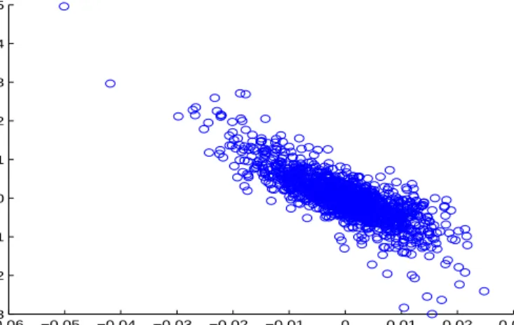
These models are based on diffusion dynamics where market variables are driven by a multidimensional Brownian motion. Recent price history across most asset classes has pointed to the importance of discontinuities in the evolution of prices; this anecdotal evidence is supplemented by an in-creasing body of statistical evidence for jumps in price dynamics [1, 2, 3, 17]. Volatility indices such as the VIX have exhibited, especially during the re-cent crisis, large fluctuations which strongly point to the existence of jumps, or spikes, in volatility. Figure 1, which depicts the daily closing levels of S&P 500 and the VIX volatility index from September 22nd, 2003 to Febru-ary 27th, 2009, reveals to the simultaneity of large drops in the S&P 500 with spikes in volatility, which corresponds to the well-known “leverage ef-fect”. Comparing the relative changes in the two series (Figure 2) reveals that, while there is already a negative correlation in small changes in the series, large changes –jumps– exhibit an even stronger negative correlation, close to -1 (see Table 1). These observations are confirmed by a recent study of Tauchen and Todorov [27], who find significant statistical evidence of simultaneous jumps of opposite sign in the VIX and the underlying in-dex. These empirical facts need to be accounted for in a realistic model for variance swap dynamics. They are also important from a pricing per-spective: Broadie and Jain [9] find that, for a wide range of models and parameter specifications, the effect of discrete sampling on the valuation of volatility derivatives is typically small while the effect of jumps can be significant. Jumps in volatility are also important in order to produce the positive “skew” of implied volatilities of VIX options [6, 21].

1.1 Contribution

Following the approach proposed by Bergomi [5, 7, 6], the present work proposes an arbitrage-free modeling framework for the joint dynamics of forward variance swap rates along with the underlying index, which

1. captures the information in index option prices by matching the index implied volatility smiles.

2. is capable of reproducing any observed term structure of variance swap rates.

3. captures the information in options on VIX futures by matching their prices/ implied volatility smiles.

4. implies a realistic joint dynamics of spot and forward implied volatili-ties, allowing in particular for jumps in volatility and returns.

5. allows for the spot/volatility correlation and the implied volatility skews (of vanilla options) to be parametrized independently.

(6)

6. is able to handle the term structure of vanilla skew separately from the term structure of volatility of volatility.

7. is tractable and enables efficient pricing of vanilla options, which is a key point for calibration and implementation of the model.

We address these different issues, while retaining tractability, by introducing a common jump factor which affects variance swaps and the underlying index with opposite signs. Describing these jumps in terms of a Poisson random measure leads to an analytically tractable framework, where VIX options

and calls/puts on the underlying index can be simultaneously priced using Fourier-based methods. Our framework is in fact a class of models and allows for various specifications of the jump size distribution; we give two worked-out examples and detail their implementation.

The difference between our modeling framework and the Bergomi model [7] is mainly the ability to meet points 5), 6) and 7) above. Also, thanks to a semi-analytic representation of call option prices, our model also satisfies the tractability property 1), allowing efficient calibration to the whole implied volatility surface. This is an advantage over the Bergomi model where only the short-term implied volatility smile can be matched [5, 7].

600 700 800 900 1000 1100 1200 1300 1400 1500 1600

22-Sep-03 25-May-04 27-Jan-05 29-Sep-05 05-Jun-06 07-Feb-07 10-Oct-07 13-Jun-08 17-Feb-09 Date S& P 50 0 5 15 25 35 45 55 65 75 85

22-Sep-03 25-May-04 27-Jan-05 29-Sep-05 05-Jun-06 07-Feb-07 10-Oct-07 13-Jun-08 17-Feb-09 Date

VI

X

Figure 1: Time series of the VIX index (bottom) depicted together with the S&P 500 (top) covering the period from September 22nd, 2003 to February 27th, 2009.

1.2 Outline

Section 2 describes variance swap contracts, forward variance swap rates and options on variance swaps. The model is described in Section 3 and two

(7)

−0.06 −0.05 −0.04 −0.03 −0.02 −0.01 0 0.01 0.02 0.03 −0.3 −0.2 −0.1 0 0.1 0.2 0.3 0.4 0.5

Figure 2: Daily relative changes in the VIX (vertical axis) vs daily relative changes in the S&P 500 index (horizontal axis), September 22nd, 2003 to February 27th, 2009.

Table 1: Conditional correlations between the daily returns on S&P 500 and the VIX from September 22nd, 2003 to February 27th, 2009.

Abs. Return Unconditional <0.5% >0.5% <1% >1% <5% >5% Correlation -0.74 -0.45 -0.78 -0.66 -0.79 -0.76 -0.93 Observations 1368 677 691 1031 337 1348 20

(8)

model specifications are presented. Section 4 discusses the VIX index and the connection between forward variance swap rates and VIX index futures. Section 5 implements the two specifications of the model and examines their performance in jointly matching VIX options and options on the S&P 500. Section 6 concludes.

2

Variance Swaps and Forward Variances

Consider an underlying asset whose priceSis modeled as a stochastic process (St)t≥0 on a filtered probability space

Ω,_F,_{Ft}t≥0,P

, where _{Ft}t≥0

represents the history of the market. We assume the market is arbitrage-free and prices of traded instruments are represented as conditional expectations with respect to an equivalent pricing measure Q. We shall neglect in the sequel corrections due to stochastic interest rates.

2.1 Variance Swaps

The annualized realized variance of a (price) process S over a time grid

t=t0 < ... < tk=T is given by RVt,T = M k k X i=1 log Sti Sti−1 2 , (1)

whereM is the number of trading days per year.

A variance swap (VS) with maturity T initiated at t < T pays the difference between the annualized realized variance of the log-returns RVt,T

less a strike called the variance swap rate VT

t , determined such that the

contract has zero value at the time of initiation t.

For any semimartingaleS, as supi=1,...,k|ti−ti−1| →0 the realized

vari-ance converges to the quadratic variation of the log price:

k X i=1 log Sti Sti−1 2 Q −→[logS]_T ₋[logS]_t .

Approximating the realized variance by the quadratic variation of the log returns is justified when the sampling frequency is daily, as is the case in most variance swap contracts, to warrant replacing the realized variance by its continuous counterpart [9]. The fixed leg paid in a variance swap is then approximated by

V_tT = 1

T₋tE([logS]T −[logS]t| Ft) , (2)

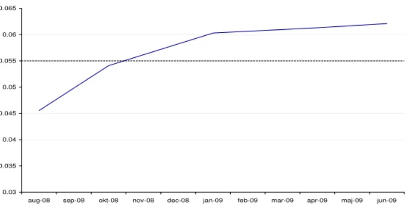
and we refer to this quantity as the (spot) variance swap (VS) rate prevailing at datetfor the maturityT. An example of a variance swap term structure is given in Figure 3.

(9)

0.03 0.035 0.04 0.045 0.05 0.055 0.06 0.065

aug-08 sep-08 okt-08 nov-08 dec-08 jan-09 feb-09 mar-09 apr-09 maj-09 jun-09

Figure 3: The term structure of 1 month forward variance swaps for the S&P 500 on August 20th, 2008.

2.2 Forward Variances

The forward variance, quoted at date t for the period [T1, T2] is the strike

that sets the value of a forward variance swap running fromT1 toT2 to zero

at timet; it is given by VT1,T2 t = 1 T2−T1 E [logS]_T₂₋[logS]_T₁ _{| F}t (3) = (T2−t)V T2 t −(T1−t)VtT1 T2−T1 , (4)

wheret < T1 < T2. The last equality follows easily by substitution of (2). In

particular, as noted in [5, 6] forward variances have the martingale property under the pricing measure.

Choosing t < s < T1 < T2 it follows by substitution of (3) and the use

of the law of iterated expectations that E VT1,T2

s | Ft=VtT1,T2 (5)

which shows that forward variances are martingales under the pricing mea-sure Q.

Assume that a set of settlement dates is given

T0 < T1< ... < Tn

known as the tenor structure and that the interval between two tenor dates is fixed,τi =Ti+1−Ti =τ (equal to 30 days if we use the tenor structure

of the VIX futures). We define theforward variance over the time interval [Ti, Ti+1] as

V_ti =VTi,Ti+1

(10)

2.3 Options on Forward Variance Swaps

A call option with strike K and maturity T1 on a forward variance swap

for the period [T1, T2] gives the holder the option to enter at date T1 into

a variance swap running from T1 to T2 with some predetermined strike K.

Hence, the value at time T1 is

π(T1, T1, T2, K) = e− RT₂ T₁ rsds_E₍_RV T1,T2−K| FT1) + =e− RT₂ T₁ rsds_VT1,T2 T1 −K + , (7)

which gives us the timetvalue

π(t, T1, T2, K) =e− RT₂ t rsds_E_VT1,T2 T1 −K + | Ft . (8) From this expression it is clear that having tractable dynamics for the for-ward variance swap rates enable the pricing of options on variance swaps.

3

A Model for the Joint Dynamics of Variance

Swaps and the Underlying Index

Our goal is to construct a model which

• allows for an arbitrary initial variance swap term structure.

• allows to specify directly the dynamics of the observable forward vari-ance swapsVti on a discrete tenor of maturities (Ti, i= 1..n).

• allows for flexible modeling of the variance swap curve: for example, it should be able to accommodate the fact that variance swaps at the long end of the maturity curve have a lower variability than those at the short end.

• allows for jumps in volatility [27] and in the underlying asset [1, 2, 3, 17].

• allows for a flexible specification of the spot price dynamics.

• is analytically tractable i.e. leads to efficient numerical methods for pricing/calibration of calls/puts both on the underlying and volatility derivatives such as options on forward variance swaps and options on forward volatility.

In order to achieve these goals, we first specify the dynamics of (a discrete tenor of) forward variance swaps (Section 3.1) using an affine specification

(11)

which allows Fourier-based pricing of European-type volatility derivatives. Once the dynamics of forward variance swaps has been fixed, we specify a jump-diffusion dynamics for the underlying asset which is compatible with the variance swap dynamics (Section 3.2). Presence of a jump component as well as a diffusion component in the underlying asset allows us to satisfy this compatibility condition while simultaneously matching values/implied volatilities of options on the underlying asset (Section 3.3).

3.1 Variance Swap Dynamics

Given that the forward variance swap rate is a (positive) martingale under the pricing measure, we model it as

V_ti=V₀ieXti =V₀iexp Z t 0 µi_sds+ Z t 0 ωe−k1(Ti−s)_dZ s+ Z t 0 Z R e−k2(Ti−s)_xJ₍_{dx ds}₎ , (9) whereJ(dxdt) is a Poisson random measure with compensatorν(dx)dtand

Z a Wiener process independent ofJ. The martingale condition imposes

µi_t=₋1 2ω 2_e−2k1(Ti−t) − Z R expne−k2(Ti−t)_xo −1ν(dx) . (10)

For t > Ti we let Vti = VTii. This specification allows for jumps and the

exponential functions inside the integrals allow to control the term structure of volatility of volatility. For example, ifk1is large andk2small, the diffusion

Zresults mostly in fluctuations at the short end of the curve, while the jumps impact the entire variance swap curve. Correlated Brownian factors can be added if more flexibility in the variance swap curve dynamics is desired, e.g. correlation between movements in the short and the long end of the curve. Likewise, functional forms other than exponentials can be used in (9), although the exponential specification is quite flexible as we will observe in the examples.

Expressions such as (8) can be evaluated using Fourier-based methods [13, 24, 18] given the characteristic function ofXi

Ti, which in this case has a

simple form:1 EheiuXiTi i = exp −1₂u2 Z Ti 0 ω2e−2k1(Ti−s)_ds₊_iu Z Ti 0 µisds + Z Ti 0 Z R expniue−k2(Ti−s)_xo −1ν(dx)dt . (11)

1_{We hope that the reader will not confuse the complex number}_i_{with the index in the}

forward variance swap rateVi t.

(12)

3.2 Dynamics of the Underlying Asset

Once the dynamics of forward variance swaps Vi

t for a discrete set of

ma-turitiesTi, i= 1..nhas been specified, this imposes some constraints on the

(risk neutral) dynamics of the underlying asset (St)t≥0. S should be such

that

1. the discounted spot price ˆSt= exp(−R₀t(rs−qs)ds)St is a (positive)

martingale, whereqt is the dividend yield.

2. the dynamics of the spot price is compatible with the specification of Vi

t, which puts the following constraint on the quadratic variation

process [lnS] of the log-price:

E[ [lnS]Ti+1−[lnS]Ti |Ft] =V

i

t (12)

To these constraints we add a third requirement, namely that: 3. the model values of calls/puts on S match the observed prices across

strikes and maturities.

Typically we need at least two distinct parameters/degrees of freedom in the dynamics of the underlying asset in order to accommodate points 2) and 3) above.

The Bergomi models [5] and [7] propose to achieve this by introducing a random ”local volatility” function which is reset at each tenor date and chosen such at timeTi to match the observed value of V_Ti_i. This procedure

guarantees coherence between the variance swaps and the underlying asset dynamics but leads to a loss of tractability: even vanilla call options need to be priced by Monte Carlo simulation for maturitiesT > T1.

We adopt here a different approach which allows a greater tractability while simultaneously allowing for jumps in the volatility and the price. In fact, as we will see, introducing jumpsisthe key to tractability.

The underlying asset is driven by

• a Brownian motion W, correlated with the diffusion component Z

driving the variance swaps: < W, Z >t=ρ t.

• a jump component, which is driven by the same Poisson random measure J which drives jumps in the variance. However, we allow different jump amplitudes in the underlying and the forward variance. Presence of a jump component as well as a diffusion component in the un-derlying asset allows us to satisfy this compatibility condition while simul-taneously matching values/implied volatilities of options on the underlying asset (Section 3.3).

For each interval [Ti, Ti+1) we introduce a stochastic diffusion coefficient

(13)

underlying asset in terms of the jump sizexin forward variance levelVi_and

Vi _{itself. We will give in section 3.4 some simple and flexible specifications}

for this function ui but most developments below hold for arbitrary choice

ofui.

We will present here the detailed computations in the (typically useful) case whereT =Tm, for m= 1, ..., n, but the analysis can be easily

general-ized to any maturity. The dynamics of the underlying asset is then specified as STm=S0exp (Z Tm 0 (rs−qs)ds+ m_X−1 i=0 µi(Ti+1−Ti) +σi WTi+1−WTi + m_X−1 i=0 Z Ti+1 Ti Z R ui x, VTii J(dx ds) ) , (13) where µi = −1₂σ2i − R R eui x,Vi Ti −1

ν(dx) and the σis are stochastic

and revealed at timeTi by relation (16) below to match the known variance

swap valueVi

Ti at this time point. The drift term µi is also stochastic and

FTi-measurable. The random jump measureJ in the index dynamics is the

same as that in the VS dynamics, so the index and the variance swaps jump simultaneously. ui is a deterministic function ofx andV_Ti_i chosen to match

the observed volatility smiles implied by prices of options on the spot. W is correlated with Z with a correlation ρ.

As far as pricing of vanilla instruments is concerned, the model can be viewed simply as a flexible (and analytically tractable) parameterization of the joint distribution of forward variance swap rates and the underlying asset on a set of tenor dates. At this level the only assumption we are making is that this joint distribution is infinitely divisible [26] and our model is just a flexible parameterization of the L´evy triplet of the distribution. This makes it particularly easy to price any payoff which involves these variables only at tenor dates.

The assumption of a common jump factor which affects the variance swaps and the underlying in opposite directions is not only analytically con-venient but quite realistic from an empirical perspective. As revealed in Table 1, while the unconditional correlation of daily returns of the VIX in-dex and the S&P 500 from September 22nd, 2003 to February 27th, 2009 is ₋74%, the conditional correlation between the two sub-series for daily moves in the S&P 500 less than 0.5% drops to ₋0.45 while the conditional correlation of moves greater than 5%, which can be interpreted as jumps, is

−93%, close to -100%. This observation is also in agreement with the find-ings reported by Tauchen and Todorov [27] using non-parametric methods. This feature, which has no equivalent in diffusion-based stochastic volatility models such as [7, 21], is a generic property of our framework.

(14)

Given the dynamics (13) of the underlying asset, the quadratic variation over the time interval [T0, Tm] is given by

[logS]_T_m₋[logS]_T₀ = m_X−1 i=0 σ_i2(Ti+1−Ti) + Z Ti+1 Ti Z R ui x, VTii 2 J(ds dx) . (14) By taking expectation on (14) the variance swap rate in (2) equals

VTm T0 = m_X−1 i=0 Ti+1−Ti Tm−T0 Eσ_i2_{| F}T0 +E Z R ui x, VTii 2 ν(dx)_{| F}T0 , and the forward variance at timet for the interval [Ti, Ti+1] equals

V_ti=Eσ_i2 _{| F}t +E Z R ui x, VTii 2 ν(dx)_{| F}t . (15)

Equation (15) has to hold at all times, but sinceVi

t is a martingale we just

need to ensure that at time Ti

V_Ti_i =σ2_i + Z R ui x, VTii 2 ν(dx) . (16) Having fixed ν(dx) it is seen that any observed forward variance structure can be matched by an appropriate choice of theσis which leaves the

param-eters inui free to calibrate to option prices.

3.3 Pricing of Vanilla Options

Let us now explain the procedure for pricing European calls and puts on S

in this framework. The aim is to compute in an efficient manner the value of call options of various strikes and maturities at, some initial datet= 0:

C(0, S0, K, Tm) =e− RTm 0 rsds_E_[(_S Tm−K) +_|F 0]. (17)

Denote by _F_t(Z,J) the filtration generated by the Wiener processZ and the Poisson random measureJ. By first conditioning on the factors driving the variance swap curve and using the iterated expectation property

C(0, S0, K, Tm) =e− RTm 0 rsds_E_[_E_[(_S Tm −K) +_|F(Z,J) Tm ]|F0] (18)

we obtain amixing formula for valuing call options:

Proposition 1 The value C(0, S0, K, Tm) of a European call option with maturity Tm and strike K is given by

(15)

where CBS₍_{S, K, T}_;_σ₎ _{denotes the Black-Scholes formula for a call option} with strike K and maturity T:

σ_∗2 = 1 Tm m_X−1 i=0 σi2 1−ρ2 (Ti+1−Ti), (20) andUTm is a F (Z,J)

Tm -measurable random variable given by

UTm =S0exp (_m₋₁ X i=0 − 1 2σ 2 iρ2+ Z R eui x,Vi Ti −1 ν(dx) (Ti+1−Ti) ρ ZTi+1−ZTi σi+ Z Ti+1 Ti Z R ui(x, VTii)J(dx ds) (21)

and the expectation in (19) is taken with respect to the law of(Z, J).

Proof. Conditional on _F_T(Z,J_m ), the increments of Z and the paths of the variance swap rates, and in particular Vi

Ti, thus the corresponding σi are

known for i= 0,1, ..., m from equation (16). Moreover

WTi+1−WTi d =ρ ZTi+1−ZTi +p(1₋ρ2₎_Wˆ Ti+1−WˆTi , where the Wiener processesZ and ˆW are independent. The processStcan

therefore be decomposed as STm=UTmexp (Z Tm 0 (rs−qs)ds+ m_X−1 i=0 −1₂σ2_i 1₋ρ2(Ti+1−Ti) +σi p 1₋ρ2_Wˆ_T i+1−WˆTi o , whereσ_i2 =Vi Ti− R Rui x, VTii 2 ν(dx) and UTm =S0exp (_m₋₁ X i=0 − 1 2σ 2 iρ2+ Z R eui x,Vi Ti −1 ν(dx) (Ti+1−Ti) ρ ZTi+1−ZTi σi + Z Ti+1 Ti Z R ui(x, VTii)J(dx ds)

is_F_T(Z,J_m )-measurable. In distribution we have

STm

d

=UTme

RTm

(16)

whereσ∗ is given in (20) and µ∗= 1 Tm m_X−1 i=0 −1₂σ_i2 1₋ρ2(Ti+1−Ti), (22)

where we notice that µ∗ = −1₂(σ∗)2. Hence, given FT(Z,Jm ), the inner

con-ditional expectation in (18) reduces to the evaluation of the Black-Scholes formula E[(STm−K)+|F (Z,J) Tm ] =C BS₍_U Tm, K, Tm;σ∗) ,

whereσ∗ depends on all theuis through (16) and (20).

This result has interesting consequences for pricing and calibration of vanilla contracts. Note that the outer expectation can be computed by Monte Carlo simulation of theZ and J: withN simulated sample paths for

Z andJ we obtain the following approximation

ˆ CN = 1 N N X k=1 CBSU_T(k_m), K, Tm;σ∗(k) _N_→∞ → C(0, S0, K, Tm) . (23)

Since the averaging is done over the variance swap factorsZ and J, this is a deterministic function of the parameters in theuis. This will prove useful

when calibrating the model using option data, since wedo not have to run theN Monte Carlo simulations for each calibration trial.

Equation (23) thus allows to calibrate the model to the entire implied volatility surface in an efficient manner, in contrast to the Bergomi model where it is only possible to calibrate to at-the-money slopes of the implied volatilities (ATM skews).

3.4 Examples

Different classes of models in the above framework can be obtained by vari-ous parameterizations of the L´evy measureν(dx) describing the jumps and for the functions ui appearing in (13). In this paper we implement two

model parameterizations; normal jumps and double exponential jumps in the variance swaps and the index.

3.4.1 Normally Distributed Jumps

In the first example, we specify the L´evy measure as

ν(dx) =λ 1 δ√2πe

−(x−₂_δm₂)2

dx, (24)

where m and δ2 _{is the mean and variance in a normal distribution and} _λ

(17)

in (11) can be calculated (see (41) in Appendix A) and prices of options on the variance swaps can be computed by Fourier transform methods.

We now consider the following specification for ui, which relates the

jumps in the variance swap to the jumps in the underlying asset

ui x, VTii = V i Ti Vi 0 !1 2 bix , (25)

but any functional form can be used as long as (16) leads to positive values forσi.

This gives us the σis at timeTi

σ2_i =V_Ti_i₋ V i Ti Vi 0 Z R (bix)2ν(dx) =V_Ti_i₋λV i Ti Vi 0 b2_im2+b2_iδ2.

In order to achieve non-negative values forσ2

i we require

λ b2_im2+b2_iδ2_≤V₀i. (26)

3.4.2 Exponentially Distributed Jumps

To introduce an asymmetry in the tail of the jump size distribution we can use a double exponential distribution [23]:

ν(dx) =λpα+e−α+x1x≥0+ (1−p)α−e−α−|x|1x<0

dx, (27) where p denote the probability of a positive jump, 1/α+ and 1/α− the

expected positive and negative jump sizes, respectively. In this specification the characteristic function for the forward variance swap is given by (43).

As above, we specify the ui function as in (25), which gives rise to the

following constraint on theσis

σ_i2 =V_Ti_i₋λV i Ti Vi 0 2pb2 i α2 + + 2 (1−p)b 2 i α2 − . To ensure positiveσis we constrain the calibration by

λ 2pb2 i α2 + +2 (1−p)b 2 i α2 − ≤V₀i. (28)

The parameters bi in the above specifications can take any value as long

as (26) respectively (28) are satisfied. We will see later, how the calibration of bi entails that jumps in the underlying have opposite direction to the

(18)

jumps in the VIX futures. Together with negative correlation between Z

and W, this feature enables the model to generate positive skews for the implied volatility of VIX options and negative skews for the implied volatil-ity of calls and puts on the underlying index, as observed in empirical data. This property is achieved without the need to add extra volatility factors, as proposed recently in e.g. [10, 20, 21] where multi-factor mean-reverting dy-namics on volatility and volatility of volatility are imposed to accommodate this behavior, resulting in a loss of tractability.

3.5 Impact of Jumps on the Valuation of Variance Swaps

As noted above, recent price history across most asset classes has pointed to the importance of discontinuities in the evolution of prices; this is sup-plemented by an increasing body of statistical evidence for jumps in price dynamics [1, 2, 3, 17]. Before moving on we would like to digress on the effect of jumps in the underlying index dynamics when pricing variance swaps.

As noted by Neuberger [25], if the underlying asset follows continuous dynamics, its quadratic variation and hence also the payoff from a variance swap can be replicated by continuous rebalancing of a position in the un-derlying asset and a static position in a log contract, which in turn can be replicated by a static portfolio of calls and puts [12, 19]:

1 T₋t([logS]T −[logS]t) = 2 T ₋t Z T t dSt St − logST St

and then under discrete sampling

M k k X i=1 log Sti Sti−1 2 = 2M k k X i=1 ∆Si Si−1 − log Si Si−1 .

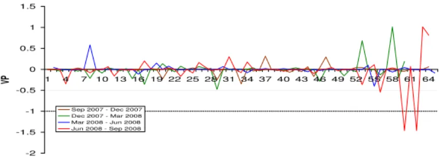
The left hand side is the realized variance paid and the right hand side is the payoff from the hedging strategy. Figure 4 depicts the day to day profit-loss from holding a long position in the replicating portfolio and a short position in the three month variance swap. Variance Point (VP) is defined as realized variance multiplied by 10,000. As can be seen, the replicating portfolio performs relatively well most of the days, but days in which the index moved considerably show an error of up to -1.5 VP. Table 2 shows the error from holding the portfolio relative to the realized variance over the three month period. The maximum error from following this strategy arises in the June 2008 - September 2008 variance swap and results in an error of

−0.243%. These four real examples indicate that the error from assuming continuous dynamics have been historically small.

Sometimes this is taken as an argument that jumps are not significant when variance swaps are priced. This can very well be a false conclusion,

(19)

which can be realized from the following. When assuming continuous dy-namics, the error that arises when valuing variance swap rates is given [14] by − 2 T₋tE Z T t Z R ey₋1₋y₋y 2 2 ν(dy)ds_{| F}t ,

where y is the jump size in the index. That this expectation is small un-der the physical measure does not entail that the mean of the error unun-der thepricing measure should be zero. This common fallacy is akin to saying that since crashes occur infrequently deep out-of-the-money puts should be priced at zero: recent experience shows that such mistaken assertions can be costly. In fact adding jumps with negative mean value to the log-price dynamics should increase the value of the variance swap rate, since being long a variance swap can be seen as an insurance against downward move-ments in the underlying asset and therefore have a risk premium attached to it [15].

4

The VIX Index

As mentioned, the market for options on the VIX index is well developed, and unless data on options on variance swaps is available, information stem-ming from this market should be used when the dynamics of the variance swaps are specified. For completeness we describe the VIX index in the first subsection, but the reader is referred to [16] and [14] for a detailed dis-cussion. In the second subsection we derive our choice for the VIX futures dynamics given the dynamics of the forward variance swaps .

4.1 Description

The Chicago Board Options Exchange (CBOE) introduced the volatility index, VIX, in 1993, and it has since become the industry benchmark for market volatility. The VIX index provides investors with a quote on the expected market volatility over the next 30 calendar days. In September 2003 the VIX was revised such that the index is now calculated on the basis of put and call options on S&P 500 instead of the S&P 100 index. Furthermore, the index was changed to calculate the expected volatility on the basis of options in a wide range of strike prices, where the original VIX index was based on at-the-money strikes only.

The general formula used in the VIX calculation at time tis

V S_tT = 2 T₋t X i ∆Ki K2 i erTt(T−t)_Q₍_K i, T;t)− 1 T₋t Ft K0 − 1 2 , (29) whereT is time of expiration,Ki the strike price of theith out-of-the money

(20)

option, ∆Ki the resolution of the strike grid:

∆Ki =

Ki+1−Ki−1

2 .

For the lowest strike, ∆Ki is the difference between the lowest and second

lowest strikes. This also applies to the highest strike. rT

t is the risk-free

interest rate to expiration, Q(Ki, T;t) the midpoint between the bid and

ask prices on the option with strike Ki and maturity T, either a call if

Ki > Ft or a put if Ki < Ft, where Ft is the forward S&P 500 index price.

K0 is the first strike below the forward index levelFt. Normally, no options

will expire in exactly 30 days. Therefore, CBOE interpolates betweenV ST1

t and V ST2 t V IXt= 100 s 365 30 (T1−t)V StT1 NT2 −30 NT2−NT1 + (T2−t)V StT2 30₋NT1 NT2 −NT1 , (30) whereNT1 and NT2 denote the actual number of days to expiration for the

two options maturities, NT1 <30< NT2.

The VIX is often presented as an indicator of the expected volatility over the next 30 days. It is not immediately clear from either (29) or (30) that this is in fact the case. For notational simplicity assume that the jumps exhibit finite variation. Then it can be shown that the realized variance of returns can be decomposed into three components

[logS]_T ₋[logS]_t= 2 T ₋t Z Ft 0 1 K2 (K−ST) +_dK + Z ∞ Ft 1 K2(ST −K) +_dK₊Z T t 1 Fs− − 1 Ft dFs − Z T t Z R ey₋1₋y₋y 2 2 J(dy ds) , (31) where J is a Poisson random measure with L´evy measure ν(dx), driving the jumps in the underlying asset. Notice how the realized variance can be replicated by trading in options and futures up to a discontinuous jump component.

Taking expectations with respect to the pricing measure in (31) we obtain

VtT = 2 T₋te RT t rsds Z ∞ 0 Q(K, T;t) K2 dK −_T2 −tE Z T t Z R ey₋1₋y₋ y 2 2 ν(dy)ds_{| F}t . (32) Equation (29) is a discretization of the first term in (32). The extra term

1 T−t Ft K0 −1 2

(21)

The square of the VIX index is thus a model free estimate of the expected volatility over the next 30 days given continuous dynamics of the underlying but under general price processes the error term is given by the last term in (32): V IX_t2 =V_tt+30days+ 2 T₋tE Z T t Z R ey₋1₋y₋y 2 2 ν(dy)ds_{| F}t . (33) 4.2 VIX Futures Let V IXi

t denote the VIX futures price for the interval [Ti, Ti+1] seen at

timet. For t=Ti we have

V IX_Ti_i2 =V_Ti_i+ 2 Z R (eui x,Vi Ti −1₋ui x, VTii −ui x, V i Ti 2 2 )ν(dx) . We also have the martingale property for t < Ti

V IX_ti =EV IX_Ti_i_|Ft

By Jensen’s inequality for convex functions

V IXti 2 ≤Eh V IXTii 2 |Ft i =V_ti+ 2E "Z R eui x,Vi Ti −1₋ui x, VTii −ui x, V i Ti 2 2 ν(dx)| Ft # , (34) since Vi

t is a martingale. Equation (34) shows that there is a “convexity

correction” connecting VIX futures to forward variance swap rates.

To obtain a tractable framework, we first characterize the dynamics of

p

Vi

t then propose an approximation which has a closed-form characteristic

function.

Proposition 2 The process pVi

t has the multiplicative decomposition

q Vi t = q Vi 0MtiAit where Ai

t is a finite variation process and Mti is an exponential martingale given by M_ti = exp Z t 0 ηi_sds+1 2 Z t 0 ωe−k1(Ti−s)_dZ s+ Z t 0 Z R 1 2e −k2(Ti−s)_xJ₍_{dx ds}₎ , (35) where ηit=− 1 8ω 2_e−2k1(Ti−t) − Z R exp 1 2e −k2(Ti−t)_x −1 ν(dx). (36)

(22)

The proof of this result is given in Appendix B. Using this result we approximateV IXi

t with

V IXi

t 'V IX0iMti =V IX0iexp(Yti) . (37)

whereYi

t = lnMti. This approximation leaves the initial level of theV IXi

and the volatility of V IXi _{untouched and thus is relevant for pricing VIX}

derivatives. As in the case of the forward variance swaps, once the L´evy measure ν(dx) is specified, the characteristic function for the exponent in (37) can be easily computed, so options on the VIX index can be priced by Fourier transform methods.2

5

Implementation

In this section the model specifications described in Section 3.4 are imple-mented on data on the VIX and the S&P 500 implied volatility smiles.

5.1 Data

We assess the performance of the model using prices from August 20th, 2008 on a range of VIX put and call options for five maturities, VIX futures for the same maturities, the dividend yield on S&P 500, call and put options on S&P 500 for six maturities and for the various maturities we also have the corresponding prices of the futures on S&P 500, from which we also derive a discount curve. We also observe 3 month forward variance swap rates for various maturities. The variance swap rates have been converted to forward 1 month variance swap rates by simple linear extrapolation and these are depicted in Figure 3. Options for which the bid price is zero were removed.

5.2 Calibration

The calibration of the model consists of three steps:

1. Determine the parameters controlling the variance swap dynamics by calibration to VIX options using the characteristic function in (42) or (44) and Fourier transform methods.

2. Use the parameters from the first step to simulate N paths of the variance swaps and store the increments of Z, the jump times and jump sizes along with theVi

Tis.

3. Calibrate to options on the index recursively by use of (23).

2_{The characteristic functions for the specifications in Section 3.4 are given in Appendix}

(23)

In the first step we compute model prices by the fast Fourier transform technique described in [13] using the revised method in [18]. The calibration is performed by minimizing the sum of squared errors weighted by the inverse bid-ask spread across all maturities and strikes on out-of-the-money options on the VIX futures

SE = X

options

1

QAsk−QBid

(QM arket,M id−QM odel)2 , (38)

using a gradient-based minimization algorithm.

The resulting parameters for the two specifications are shown in Table 3 and it also includes the resulting average relative percentage bid-ask error from the calibration,

Error = 1 #_{options_}

X

options

max(QM odel−QAsk)+,(QBid−QM odel)+

QM arket,M id

. (39) We see how both model specifications are able to achieve very low calibration error. Note the high value of k1 compared to k2, which implies (in the

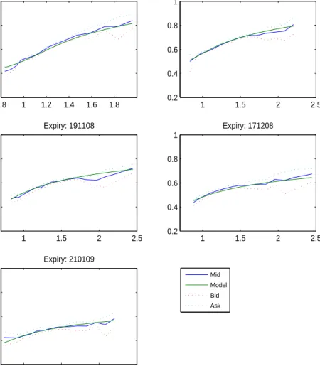
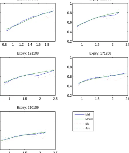
risk-neutral dynamics) that the diffusion component Z is mainly causing fluctuations at the short end of the variance swap curve, while the jumps impact the entire curve.

Figures 5 and 6 depict the (Black) implied volatility for the bid, ask, mid and model prices of VIX options as a function of moneyness. We observe that model prices fit very well within the bid-ask spread for almost all the observations in both specifications. This performance should be compared with flat model implied volatilities in the Bergomi model [5] and downward sloping volatilities in the Heston model [22]. The Bergomi model [7] is able to generate positive skews on volatility of volatility via the use of a Markov functional mapping for the forward variances, but it should be noted that the model can only price vanilla options on the underlying index by Monte Carlo simulation.

Step 2 is done by discretization of (9). In this example we have used 2_·105 _{simulated sample paths. Simulation of the jumps is straightforward,}

since they arrive at constant intensity and the jump sizes are computed by draws from a normal/exponential distribution times the scaling e−k2(Ti−τ)_,

whereτ is the jump time. For details on how to simulate the increments in the variance swaps due to the diffusion the reader is referred to [5].

In step 3 we have fixed the correlation parameter between the continuous components toρ=₋0.45.3 Then, the last step is implemented step-wise by matching the model prices (23) to market prices on the shortest maturity

3_{Instead one could also specify a correlation} _ρ

i on each interval and include that pa-rameter in the calibration for each interval. We tried this, but the performances of the models did not improve with this added flexibility.

(24)

out-of-the-money options. Again, this is achieved by minimizing the SE (38). This yields b0. Then b1 are found in the same way by calibrating to

the next maturing options by the use ofb0 for the first interval in (21). The

remainingbis are estimated in a similar manner.

The estimated parameters for the two different specifications of the jump size distributions are shown in Table 4 along with the pricing error in (39) for each maturity. The mean and standard deviations of the jumps before scaling with Vi

Ti/V

i

0

1

2 _{are also included. The values of} _b

i for i = 0, ...,3

relate to the monthly distributions of the index up to the maturity of the options expiring on December 19th, 2008. For the last two option maturi-ties the interval between the expirations are three months and hencebi for

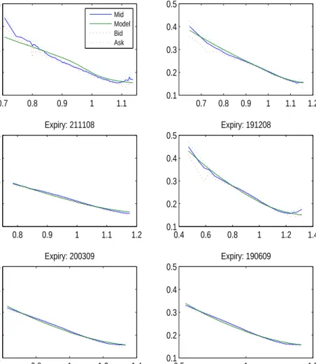
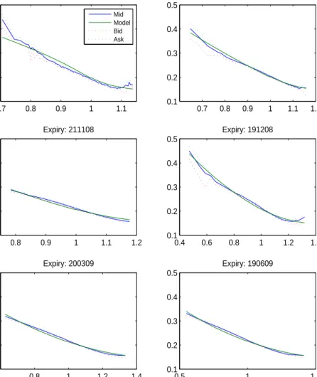
i= 4,5 relate to the three month distributions of the index. Double expo-nential jumps perform slightly better on the first interval, but there is not a strong difference between the two specifications, showing that the model performance is not very sensitive to the choice of the jump size distribution. Figures 7 and 8 show the result of the calibration to the S&P 500 options. The fit of the two specifications are practically indistinguishable and overall the calibrations perform well for both with somewhat less success on the shortest maturity.

We conclude this section with an examination of the size of the jump er-ror term when valuing the forward variance swap ratesVi _{under the}

assump-tion of continuous dynamics given the models implemented in this paper are “true”. Recall that the error is given by

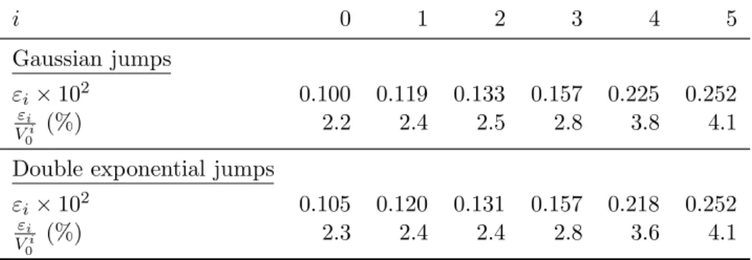
εi=−2E "Z R eui x,Vi Ti −1₋ui x, VTii −ui x, V i Ti 2 2 ! ν(dx)_{| F}0 # . (40) In Table 5 the absolute errors implied by the calibration of the two model specifications are computed for each interval. Moreover, the errors relative to the initial forward variance swap value are reported. For the first interval it is 2.2%/2.3% and then it roughly increases as iincreases. The reported errors for the last two intervals are taken as the average of the three monthly errors relative to the average of the three monthly forward variances covering the same intervals.

6

Conclusion

We have presented a model for the joint dynamics of a set of forward vari-ance swap rates along with the underlying index. Using L´evy processes as building blocks, this model leads to a tractable pricing framework for variance swaps, VIX futures and vanilla call/put options, which makes cal-ibration of the model to such instruments feasible. This tractability feature distinguishes our model from previous attempts [5, 4, 21] which only allow

(25)

for full Monte Carlo pricing of vanilla options.

Our model reproduces salient empirical features of variance swap dynam-ics, in particular the strong negative correlation of large index moves with large moves in the VIX and the positive skew observed in implied volatilities of VIX options, by introducing a common jump component in the variance swaps and the underlying asset. Using two different specifications for the jump size distribution (L´evy measure) we have illustrated the feasibility of the numerical implementation, as well as the capacity of the model to match a complete set of market prices of vanilla options and options on the VIX. Our model can be used to price and hedge various payoffs sensitive to for-ward volatility, such as cliquet or forfor-ward start options, as well as volatility derivatives, in a manner consistent with market prices of simpler instruments such as calls, puts or variance swaps which are typically used for hedging them.

References

[1] Y. Ait-Sahalia and J. Jacod,Estimating the Degree of Activity of Jumps in High Frequency Financial Data, Annals of Statistics, forth-coming, (2008).

[2] T. Andersen, L. Benzoni, and J. Lund, An Empirical Investiga-tion of Continuous-Time Equity Return Models, Journal of Finance, 57 (2002), pp. 1239–1284.

[3] O. Barndorff-Nielsen and N. Shephard,Variation, Jumps, Mar-ket Frictions and High-Frequency Data in Financial Econometrics, in Advances in Economics and Econometrics: Theory and Applications, Ninth World Congress, R. Blundell, W. K. Newey, and T. Persson, eds., Econometric Society Monographs, Cambridge Univ Press, 2007, pp. 328–372.

[4] L. Bergomi,Smile Dynamics, Risk, 17 (2004), pp. 117–123. [5] ,Smile Dynamics II, Risk, 18 (2005), pp. 67–73.

[6] ,Dynamic properties of smile models, in Frontiers in Quantitative Finance: Volatility and Credit Risk Modeling, R. Cont, ed., Wiley, 2008, ch. 3.

[7] ,Smile Dynamics III, Risk, 21 (2008), pp. 90–96.

[8] M. Broadie and A. Jain,Pricing and Hedging Volatility Derivatives, The Journal of Derivatives, 15 (2008), pp. 7–24.

(26)

[9] , The Effect of Jumps and Discrete Sampling on Volatility and Variance Swaps, International Journal of Theoretical and Applied Fi-nance, 11 (2008), pp. 761–797.

[10] H. Buehler,Consistent Variance Curve Models, Finance and Stochas-tics, 10 (2006), pp. 178–203.

[11] P. Carr, H. Geman, D. Madan, and M. Yor,Pricing Options on Realized Variance, Finance and Stochastics, 9 (2005), pp. 453–475. [12] P. Carr and D. Madan,Towards a Theory of Volatility Trading, in

Volatility: New Estimation Techniques for Pricing Derivatives, R. Jar-row, ed., Risk Publications, 1998.

[13] P. Carr and D. Madan, Option Valuation using the Fast Fourier Transform, Journal of Computational Finance, 2 (1999), pp. 61–73. [14] P. Carr and L. Wu,A Tale of Two Indices, Journal of Derivatives,

13 (2006), pp. 13–29.

[15] ,Variance Risk Premiums, Review of Financial Studies, 22 (2009), pp. 1311–1341.

[16] CBOE, VIX: CBOE Volatility Index,

http://www.cboe.com/micro/vix/vixwhite.pdf, (2003).

[17] R. Cont and C. Mancini, Nonparametric Tests for Analyzing the Fine Structure of Price Fluctuations, Financial Engineering Report 2007-13, Columbia University, 2007.

[18] R. Cont and P. Tankov,Financial Modelling with Jump Processes, Chapman & Hall/CRC, 2004.

[19] K. Demeterfi, E. Derman, M. Kamal, and J. Zou, A Guide to Volatility and Variance Swaps, Journal of Derivatives, 6 (1999), pp. 9– 32.

[20] D. Duffie, J. Pan, and K. Singleton, Transform Analysis and Asset Pricing for Affine Jump-diffusions, Econometrica, 68 (2000), pp. 1343–1376.

[21] J. Gatheral,Consistent Modeling of SPX and VIX Options, in Bache-lier Congress, July 2008.

[22] S. Heston, A Closed-Form Solution for Options with Stochastic Volatility with Applications to Bond and Currency Options, Review of Financial Studies, 6 (1993), pp. 327–343.

(27)

[23] S. Kou, A Jump-Diffusion Model for Option Pricing, Management Science, 48 (2002), pp. 1086–1101.

[24] A. Lewis, A Simple Option Formula For General Jump-Diffusion And Other Exponential L´evy Processes, tech. report, OptionCity.net, http://optioncity.net/pubs/ExpLevy.pdf, 2001.

[25] A. Neuberger, The Log Contract: A New Instrument to Hedge Volatility, Journal of Portfolio Management, 20 (1994), pp. 74–80. [26] K. Sato, L´evy Processes and Infinitely Divisible Distributions,

Cam-bridge University Press, 1999.

[27] V. Todorov and G. Tauchen, Volatility Jumps, working paper, Duke University, 2008.

(28)

A

Characteristic Functions

A.1 Normally Distributed Jumps

Variance Swaps

We have from [26] that the characteristic function ofXi

Ti is given by EheiuXTii i_{= exp} −1₂u2 Z Ti 0 ω2e−2k1(Ti−s)_ds₊_iu Z Ti 0 µi_sds + Z Ti 0 Z R expniue−k2(Ti−s)_xo −1ν(dx)dt . Notice now that _Z

Ti 0 e−2k1(Ti−s)_ds₌ 1−e −2k1Ti 2k1 and EeY=em+δ22

forY _∼N m, δ2. Inserting this into the expression for the characteristic function we arrive at EheiuXTii i_{= exp} −1₂ω2iu1−e −2k1Ti 2k1 − 1 2ω 2_u21−e−2k1Ti 2k1 −iuλ Z Ti 0 exp e−k2(Ti−s)_m₊1 2e −2k2(Ti−s)_δ2 −1 ds +λ Z Ti 0 exp iue−k2(Ti−s)_m −1 2u 2_e−2k2(Ti−s)_δ2 −1 ds . (41) VIX Futures

Recall from (37) that V IXti 'V IX0iMti where Mti = exp(Yti) is a positive

exponential martingale. The characteristic function of

Y_Ti_i = Z Ti 0 η_sids+1 2 Z Ti 0 ωe−k1(Ti−s)_dZ s+ Z Ti 0 Z R 1 2e −k2(Ti−s)_xJ₍_{dx ds}₎

can be found in the same way as for Xi_{. It is given by}

EheiuY i Ti i = exp −1₈ω2iu1−e −2k1Ti 2k1 − 1 8ω 2_u21−e−2k1Ti 2k1 −iuλ Z Ti 0 exp 1 2e −k2(Ti−s)_m₊1 8e −2k2(Ti−s)_δ2 −1 ds +λ Z Ti 0 exp 1 2iue −k2(Ti−s)_m −1₈u2e−2k2(Ti−s)_δ2 −1 ds . (42)

(29)

A.2 Exponentially Distributed Jumps

Variance Swaps

The characteristic function in (11) takes the form EheiuXTii i = exp −1 2ω 2_iu1−e−2k1Ti 2k1 − 1 2ω 2_u21−e−2k1Ti 2k1 −iuλ Z Ti 0 pα+ α+−e−k2(Ti−s) + (1−p)α− α−+e−k2(Ti−s) − 1 ds +λ Z Ti 0 pα+ α+−iue−k2(Ti−s) + (1−p)α− α−+iue−k2(Ti−s) − 1 ds . (43) VIX Futures

Recall from (37) that V IXi

t 'V IX0iMti where Mti = exp(Yti) is a positive

exponential martingale. In this specification the characteristic function of

Y_Ti_i is given by EheiuY i Ti i = exp −1₈ω2iu1−e −2k1Ti 2k1 − 1 8ω 2_u21−e−2k1Ti 2k1 −iuλ Z Ti 0 pα+ α+−1₂e−k2(Ti−s) + (1−p)α− α−+1₂e−k2(Ti−s) − 1 ! ds +λ Z Ti 0 pα+ α+−1₂iue−k2(Ti−s) + (1−p)α− α−+1₂iue−k2(Ti−s) − 1 ! ds ) . (44)

(30)

B

Proof of proposition 2

We can expressVi t in (9) as Vti =V0i+ Z t 0 Vsi−ωe−k1(Ti−s)dZs + Z t 0 Z R V_si₋expne−k2(Ti−s)_xo −1J(ds dx) − Z t 0 Z R V_si₋expne−k2(Ti−s)_xo −1ν(dx)ds.

Applying the Itˆo formula topVi

t we obtain q Vi t = q Vi 0 + 1 2 Z t 0 V_si₋2ω2e−2k1(Ti−s) −1₄ V_si₋−32 ds − Z t 0 Z R Vsi− expne−k2(Ti−s) xo₋11 2 V i s− −1₂ ν(dx)ds + Z t 0 V_si₋ωe−k1(Ti−s)1 2 V i s− −1₂ dZs + Z t 0 Z R V_si₋12 exp 1 2e −k2(Ti−s)_x −1 J(ds dx) = q V₀i+ 1 2 Z t 0 q Vsi−ωe−k1(Ti−s)dZs − Z t 0 Z R q Vi s− 1 2 expne−k2(Ti−s)_xo −1₋1 8ω 2_e−2k1(Ti−s) ν(dx)ds + Z t 0 Z R q Vi s− exp 1 2e −k2(Ti−s)_x −1 J(ds dx) . This can be written as

q Vi t = q Vi 0exp Z t 0 b µisds+ 1 2 Z t 0 ωe−k1(Ti−s)_dZ s (45) + Z t 0 Z R 1 2e −k2(Ti−s)_xJ₍_{dx ds}₎ , where b µi t=− 1 4ω 2_e−2k1(Ti−t) −1 2 Z R expne−k2(Ti−t)_xo −1ν(dx).

The stochastic integrals in (45) being processes with independent incre-ments, a straightforward application of the exponential formula for Poisson random measures [18, Prop. 3.6.] yields the multiplicative decomposition in Proposition 2 whereM is given by (35)-(36).

(31)

C

Tables

Table 2: Error from following the replicating strategy relative to the realized variance over the three month windows.

Sep-Dec 2007 Dec 2007-Mar 2008 Mar-Jun 2008 Jun-Sep 2008 Error ₋0.137% ₋0.025% 0.060% ₋0.243%

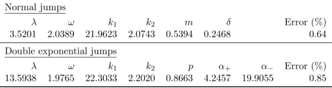
Table 3: Calibrated parameters for the two models from the VIX volatility smiles on August 20th, 2008. The top panel corresponds to the normally distributed jumps and the bottom to the double exponentially distributed jumps.

Normal jumps

λ ω k1 k2 m δ Error (%)

3.5201 2.0389 21.9623 2.0743 0.5394 0.2468 0.64 Double exponential jumps

λ ω k1 k2 p α+ α− Error (%)

(32)

Table 4: Model parameters calibrated from the S&P 500 volatility smiles on August 20th, 2008 with the correlation between the two Brownian compo-nents set to -0.45. i 0 1 2 3 4 5 Gaussian jumps bi -0.151 -0.159 -0.152 -0.173 -0.187 -0.193 bim -0.081 -0.086 -0.082 -0.093 -0.101 -0.104 |biδ| 0.037 0.039 0.038 0.043 0.046 0.048 Error (%) 8.8 0.6 1.1 1.8 1.9 2.7 Double exponential jumps

bi -0.153 -0.159 -0.149 -0.169 -0.184 -0.192 bip α+ − bi(1−p) α− -0.030 -0.031 -0.029 -0.033 -0.036 -0.038 _b2 ip α2 + + b2i(1−p) α2 − 1 2 0.034 0.035 0.033 0.037 0.040 0.042 Error (%) 6.9 0.8 1.4 2.0 2.1 2.7

Table 5: The errors arising from approximating the index dynamics with a continuous process given the model specifications described in this paper are “true”. i 0 1 2 3 4 5 Gaussian jumps εi×102 0.100 0.119 0.133 0.157 0.225 0.252 εi Vi 0 (%) 2.2 2.4 2.5 2.8 3.8 4.1

Double exponential jumps

εi×102 0.105 0.120 0.131 0.157 0.218 0.252 εi

Vi

(33)

-2 -1.5 -1 -0.5 0 0.5 1 1.5 1 4 7 10 13 16 19 22 25 28 31 34 37 40 43 46 49 52 55 58 61 64 VP Sep 2007 - Dec 2007 Dec 2007 - Mar 2008 Mar 2008 - Jun 2008 Jun 2008 - Sep 2008

Figure 4: The profit-loss from day to day in variance points (VP) from holding a long position of the hedge portfolio and a short variance swap for four different three month variance swaps. Thex-axis is trading days during the three month period.

(34)

0.8 1 1.2 1.4 1.6 1.8 0.4 0.6 0.8 1 Expiry: 170908 1 1.5 2 2.5 0.2 0.4 0.6 0.8 1 Expiry: 221008 1 1.5 2 2.5 0.2 0.4 0.6 0.8 1 Expiry: 191108 1 1.5 2 2.5 0.2 0.4 0.6 0.8 1 Expiry: 171208 1 1.5 2 2.5 0.2 0.4 0.6 0.8 1 Expiry: 210109 Mid Model Bid Ask

Figure 5: VIX implied volatility smiles on August 20th 2008 for the model with normally distributed jump sizes plotted against moneyness

(35)

0.8 1 1.2 1.4 1.6 1.8 0.4 0.6 0.8 1 Expiry: 170908 1 1.5 2 2.5 0.2 0.4 0.6 0.8 1 Expiry: 221008 1 1.5 2 2.5 0.2 0.4 0.6 0.8 1 Expiry: 191108 1 1.5 2 2.5 0.2 0.4 0.6 0.8 1 Expiry: 171208 1 1.5 2 2.5 0.2 0.4 0.6 0.8 1 Expiry: 210109 Mid Model Bid Ask

Figure 6: VIX implied volatility smiles on August 20th 2008 for the model with double exponentially distributed jump sizes plotted against moneyness

(36)

0.7 0.8 0.9 1 1.1 0.1 0.2 0.3 0.4 0.5 Expiry: 190908 0.7 0.8 0.9 1 1.1 1.2 0.1 0.2 0.3 0.4 0.5 Expiry: 171008 0.8 0.9 1 1.1 1.2 0.1 0.2 0.3 0.4 0.5 Expiry: 211108 0.4 0.6 0.8 1 1.2 1.4 0.1 0.2 0.3 0.4 0.5 Expiry: 191208 0.8 1 1.2 1.4 0.1 0.2 0.3 0.4 0.5 Expiry: 200309 0.5 1 1.5 0.1 0.2 0.3 0.4 0.5 Expiry: 190609 Mid Model Bid Ask

Figure 7: S&P 500 implied volatility smiles on August 20th 2008 for the model with normally distributed jump sizes plotted against moneynessm=

(37)

0.7 0.8 0.9 1 1.1 0.1 0.2 0.3 0.4 0.5 Expiry: 190908 0.7 0.8 0.9 1 1.1 1.2 0.1 0.2 0.3 0.4 0.5 Expiry: 171008 0.8 0.9 1 1.1 1.2 0.1 0.2 0.3 0.4 0.5 Expiry: 211108 0.4 0.6 0.8 1 1.2 1.4 0.1 0.2 0.3 0.4 0.5 Expiry: 191208 0.8 1 1.2 1.4 0.1 0.2 0.3 0.4 0.5 Expiry: 200309 0.5 1 1.5 0.1 0.2 0.3 0.4 0.5 Expiry: 190609 Mid Model Bid Ask

Figure 8: S&P 500 implied volatility smiles on August 20th 2008 for the model with double exponentially distributed jump sizes plotted against mon-eynessm=K/St on the xaxis.

(38)

Working Papers from Finance Research Group

F-2009-05

Rama Cont & Thomas Kokholm: A Consistent Pricing Model for Index

Options and Volatility Derivatives.

F-2009-04

Stefan Hirth & Marliese Uhrig-Homburg: Investment Timing, Liquidity,

and Agency Costs of Debt.

F-2009-03

Lasse Bork: Estimating US Monetary Policy Shocks Using a

Factor-Augmented Vector Autoregression: An EM Algorithm Approach.

F-2009-02

Leonidas Tsiaras: The Forecast Performance of Competing Implied

Volatility Measures: The Case of Individual Stocks.

F-2009-01

Thomas Kokholm & Elisa Nicolato: Sato Processes in Default Modeling.

F-2008-07

Esben Høg, Per Frederiksen & Daniel Schiemert: On the Generalized

Brownian Motion and its Applications in Finance.

F-2008-06

Esben Høg: Volatility and realized quadratic variation of differenced

re-turns. A wavelet method approach.

F-2008-05

Peter Løchte Jørgensen & Domenico De Giovanni: Time Charters with

Pur-chase Options in Shipping: Valuation and Risk Management.

F-2008-04

Stig V. Møller: Habit persistence: Explaining cross-sectional variation in

returns and time-varying expected returns.

F-2008-03

Thomas Poulsen: Private benefits in corporate control transactions.

F-2008-02

Thomas Poulsen: Investment decisions with benefits of control.

F-2008-01

Thomas Kokholm: Pricing of Traffic Light Options and other Correlation

Derivatives.

F-2007-03

Domenico De Giovanni: Lapse Rate Modeling: A Rational Expectation

Ap-proach.

F-2007-02

Andrea Consiglio & Domenico De Giovanni: Pricing the Option to

Sur-render in Incomplete Markets.

F-2006-09

Peter Løchte Jørgensen: Lognormal Approximation of Complex

Path-dependent Pension Scheme Payoffs.

F-2006-08

Peter Løchte Jørgensen: Traffic Light Options.

F-2006-07 David

C.

Porter,

Carsten Tanggaard, Daniel G. Weaver & Wei Yu:

Dispersed Trading and the Prevention of Market Failure: The Case of the

Copenhagen Stock Exhange.

(39)

F-2006-06

Amber Anand, Carsten Tanggaard & Daniel G. Weaver: Paying for Market

Quality.

F-2006-05

Anne-Sofie Reng Rasmussen: How well do financial and macroeconomic

variables predict stock returns: Time-series and cross-sectional evidence.

F-2006-04

Anne-Sofie Reng Rasmussen: Improving the asset pricing ability of the

Consumption-Capital Asset Pricing Model.

F-2006-03

Jan Bartholdy, Dennis Olson & Paula Peare: Conducting event studies on a

small stock exchange.

F-2006-02

Jan Bartholdy & Cesário Mateus: Debt and Taxes: Evidence from

bank-financed unlisted firms.

F-2006-01

Esben P. Høg & Per H. Frederiksen: The Fractional Ornstein-Uhlenbeck

Process: Term Structure Theory and Application.

F-2005-05

Charlotte Christiansen & Angelo Ranaldo: Realized bond-stock correlation:

macroeconomic announcement effects.

F-2005-04

Søren Willemann: GSE funding advantages and mortgagor benefits:

Answers from asset pricing.

F-2005-03

Charlotte

Christiansen:

Level-ARCH short rate models with regime

switch-ing: Bivariate modeling of US and European short rates.

F-2005-02

Charlotte Christiansen, Juanna Schröter Joensen and Jesper Rangvid: Do

more economists hold stocks?

F-2005-01

Michael Christensen: Danish mutual fund performance - selectivity, market

timing and persistence.

(40)

ISBN 9788778824271

Department of Business Studies

Aarhus School of Business Aarhus University Fuglesangs Allé 4 DK-8210 Aarhus V - Denmark Tel. +45 89 48 66 88 Fax +45 86 15 01 88 www.asb.dk