2015
Local prediction and classification techniques for
machine learning and data mining
Cory Lee Lanker
Iowa State University
Follow this and additional works at:https://lib.dr.iastate.edu/etd
Part of theStatistics and Probability Commons
This Dissertation is brought to you for free and open access by the Iowa State University Capstones, Theses and Dissertations at Iowa State University Digital Repository. It has been accepted for inclusion in Graduate Theses and Dissertations by an authorized administrator of Iowa State University Digital Repository. For more information, please [email protected].
Recommended Citation
Lanker, Cory Lee, "Local prediction and classification techniques for machine learning and data mining" (2015).Graduate Theses and Dissertations. 14404.
by
Cory L. Lanker
A dissertation submitted to the graduate faculty in partial fulfillment of the requirements for the degree of
DOCTOR OF PHILOSOPHY
Major: Statistics
Program of Study Committee: Stephen B. Vardeman, Co-Major Professor
Max D. Morris, Co-Major Professor Kris De Brabanter
Dan Nettleton Huaiqing Wu
Iowa State University Ames, Iowa
2015
DEDICATION
TABLE OF CONTENTS
LIST OF TABLES . . . vi
LIST OF FIGURES . . . vii
ABSTRACT . . . ix
CHAPTER 1. INTRODUCTION . . . 1
CHAPTER 2. A DATA-DERIVED MIXTURE PRIOR FOR PRE-DICTION BASED ON HIERARCHICAL BAYES GAUSSIAN MIX-TURE MODELS . . . 3
2.1 Introduction . . . 4
2.2 Prediction Using Mixture Models . . . 6
2.2.1 Population probability model . . . 6
2.2.2 Dirichlet process model . . . 7
2.2.3 Prior distribution . . . 7
2.2.4 Posterior distribution . . . 9
2.2.5 Prediction . . . 9
2.2.6 Tuning model parameters . . . 11
2.3 Demonstration of Our Method . . . 11
2.3.1 Predicting the doppler function . . . 12
2.3.2 Comprehensive simulation study . . . 17
2.3.3 Application to machine learning data sets . . . 27
2.4 Discussion . . . 31
2.5.1 Conditional posterior of θi . . . 34
2.5.2 Conditional posterior on µm . . . 34
2.5.3 Conditional posterior of Σm . . . 36
CHAPTER 3. CLASSIFICATION WITH A DATA-DERIVED MIX-TURE PRIOR BASED ON HIERARCHICAL BAYES GAUSSIAN MIXTURE MODELS . . . 37
3.1 Introduction . . . 38
3.2 Classification Using Mixture Models . . . 40
3.2.1 Classification problem setup . . . 40
3.2.2 Model prior specification . . . 42
3.2.3 Posterior distribution . . . 45
3.2.4 Classification . . . 49
3.3 Demonstration of Our Method . . . 51
3.3.1 Predicting the doppler function . . . 51
3.3.2 Comprehensive simulation study . . . 52
3.3.3 Application to machine learning data set . . . 65
3.4 Discussion . . . 66
3.5 Appendix: Derivation of Posterior Conditional Distribution for µm . . . . 68
CHAPTER 4. A GENERIC CLASSIFICATION ROUTINE FOR CAT-EGORICAL PREDICTORS USING LIKELIHOOD RATIO STATIS-TICS AND RANDOM FORESTS . . . 70
4.1 Introduction . . . 71
4.2 Classification Using Categorical Predictors . . . 72
4.3 Generic Classification With Likelihood Ratios . . . 75
4.4 Demonstration of Our Method . . . 78
4.4.1 Simulation study . . . 78
4.4.2 King-rook versus king-pawn data set . . . 82
LIST OF TABLES
Table 2.1 Unexplained Variation of the Doppler Function for 50 Random Seeds . . . 14
Table 2.2 Unexplained Variation of the Doppler Function With Spurious Predictor for 50 Random Seeds . . . 15
Table 2.3 Unexplained Variation of the Doppler Function With Various Scale Matrices Provided for Mixture Prior for 50 Random Seeds 16
Table 2.4 Average Computation Times, in Minutes, for the Prediction Meth-ods . . . 27
Table 2.5 R2 for Prediction of Four Machine Learning Data Sets Using Mix-ture Prior Bayes, k-Nearest Neighbors, and Random Forests . . . 27
LIST OF FIGURES
Figure 2.1 Doppler Function Test Case Data. . . 13
Figure 2.2 Comparison of Doppler Function Prediction Values. . . 14
Figure 2.3 Fewer Scale Matrices Degrades Prediction Performance. . . 16
Figure 2.4 Component Parameters During Gibbs Sampler Initialization. . . 17
Figure 2.5 Maximum Component Overlap From MixSim-Generated Data. . 19
Figure 2.6 Optimal Number of Components for the Likelihood-Based Method. 21
Figure 2.7 Optimal Number of Neighbors for k-Nearest Neighbors. . . 22
Figure 2.8 Mixture Prior Bayes Prediction Error Ratios With Comparison Methods for Comprehensive Simulation Study. . . 23
Figure 2.9 Prediction Error Ratios For Six Predictors. . . 26
Figure 2.10 Iterate Squared Error Rates for Gibbs Sample for the California Housing Data Analysis. . . 30
Figure 3.1 Classification of Data From the Doppler Function . . . 53
Figure 3.2 Simulation Study Error Ratios forp= 6 and Multivariate Normal Scenario. . . 57
Figure 3.3 Simulation Study Error Ratios forp = 6 and Spurious Predictor Scenario. . . 58
Figure 3.4 Simulation Study Error Ratios forp= 6 and Uniform X Scenario. 59
Figure 3.5 Simulation Study Error Ratios for Small-Sized Data Sets and Multivariate Normal Scenario. . . 60
Figure 3.6 Simulation Study Error Ratios for Medium-Sized Data Sets and Multivariate Normal Scenario. . . 61
Figure 3.7 Simulation Study Error Ratios for Small-Sized Data Sets and Spu-rious Predictor Scenario. . . 62
Figure 3.8 Simulation Study Error Ratios for Medium-Sized Data Sets and Spurious Predictor Scenario. . . 63
Figure 3.9 Simulation Study Computation Time. . . 66
Figure 3.10 Pairs of Predictors for Banknote Authentication Data Set. . . 67
Figure 4.1 Simulation Study Category Proportions for Different α Values. . 80
Figure 4.2 Ratio of Misclassification Error for Random Forests With Differ-ent Input. . . 81
Figure 4.3 Ratio of Misclassification Error With Sparse Data Correction Fac-tor. . . 83
ABSTRACT
A variety of conditional probability models estimate the regression or class proba-bility function for the purpose of prediction or classification. Bayesian mixture models provide flexible prediction and classification methods for modeling local linearities of the regression or class probability function. A hierarchical Bayes Gaussian mixture model is proposed that directly uses data to define a mixture prior for its Gaussian mixture com-ponent parameters. This nonparametric Bayesian mixture model uses the stick-breaking construction of a Dirichlet process model. Prediction and classification comes directly from the posterior distribution via Gibbs sampling. Comprehensive simulation studies demonstrate performance of both the regression and classification methods. Five stan-dard machine learning data sets show prediction and classification results competitive with local methods. A generic classification algorithm is outlined given categorical pre-dictors. If too many categories are present or if many interaction levels affect the class probability function, no current methods can reduce bias effectively. A proposed solu-tion is a generic way to characterize the informasolu-tion about the class probability funcsolu-tion available in the predictors through likelihood ratio statistics. This proposed classifier relies on random forests to reduce bias by utilizing all information in the generated log likelihood ratio features. A simulation study and an application data set demonstrate potential advantages of this classification method for categorical predictors.
CHAPTER 1.
INTRODUCTION
My research is in predictive analytics—the use of data to form prediction or classifica-tion values for new observaclassifica-tions. The goal of predicclassifica-tion is to form values with minimum squared error by estimating the regression function. The goal of classification is to form values with minimum misclassification error by choosing the most probable class. Most of my research extends a Bayesian model formulated in an unpublished manuscript by Ken Ryan and Stephen Vardeman in 2012. My research applies this Bayesian model to prediction and classification problems. The Ryan and Vardeman model defines a Dirich-let process clustering procedure using a mixture prior on the model’s latent Gaussian mixture parameters. Such mixture prior corrects a deficiency of multivariate Gaussian clustering procedures being too sensitive to the choice of covariance prior as noted in Gel-man et al. (2013). The model has known conditional distributions for all parameters, allowing efficient Gibbs sampling of the posterior distribution.
In my first research project, I create a flexible prediction method based on the Ryan and Vardeman model. I apply this model to prediction problems by calculating the conditional mean of the predictive posterior distribution. The provided Gibbs sampler C code had implementation problems, requiring significant changes. I wrote R code to allow comprehensive simulation studies. Prediction results are competitive with the frequentist alternative and other methods in a variety of tested scenarios. In general, this mixture prior prediction method improves prediction for small sample multivariate data with locally linear regression functions. Four standard machine learning data sets demonstrate improved prediction performance.
My second research project extends this functioning mixture prior prediction method to classification problems. Difficulties arise as I cannot simply input a binary response into a multivariate Gaussian mixture model. Instead, I create a latent Gaussian response with its own mixture prior. The most probable class comes from the resulting posterior distribution. I derived the form of the conditional distributions for the mean parameter and the latent response, and I rewrote the C code Gibbs sampler and R code for this context. A simulation study and standard data sets characterize method performance.
My third research project deals with classification with sparse categorical data. Meth-ods currently use categorical data ineffectively when there are many sparse categorical variables or the response is primarily a function of interactions between sparse cate-gorical variables. I demonstrate that using likelihood ratio statistics of the catecate-gorical counts instead of the categorical predictors improves classification performance of ran-dom forest classifiers. I offer a correction to the calculation of likelihood ratio features to prevent overfitting the classifier. This method improves classification of a standard machine learning chess classification data set.
CHAPTER 2.
A DATA-DERIVED MIXTURE PRIOR FOR
PREDICTION BASED ON HIERARCHICAL BAYES
GAUSSIAN MIXTURE MODELS
A paper in preparation
Cory L. Lanker1,2, Kenneth J. Ryan3, Mark V. Culp3, Max D. Morris1, Stephen B. Vardeman1
Abstract
A variety of conditional probability models estimate the regression function for the purpose of prediction. Bayesian mixture models provide flexible prediction methods for modeling local linearities of the regression function. We propose a hierarchical Bayes Gaussian mixture model as a flexible prediction method given continuous predictors. This paper outlines a probability model that amends a standard Bayes prediction method based on Gaussian mixture models by directly using data to define a mixture prior for its Gaussian mixture component parameters. Without this mixture prior the posterior distribution is strongly influenced by the choice of prior variance and typically yields over-smoothed estimates of the regression function. A data-derived prior circumvents this problem and gives a posterior distribution with more localized modeling of the re-gression function. This nonparametric Bayesian mixture model uses the stick-breaking 1Graduate student, Professor, and University Professor, respectively, Department of Statistics, Iowa
State University.
2Primary researcher and author.
construction of a Dirichlet process model. Prediction of the regression function comes directly from the posterior distribution via Gibbs sampling. A comprehensive simulation study demonstrates method performance with regression functions composed of a mix-ture of eight overlapping multivariate normal densities. Four standard machine learning data sets show prediction results competitive with local regression methods.
2.1
Introduction
The subject of this paper is flexible prediction for locally linear regression functions. The problem under consideration is estimation of a multivariate regression function. This paper offers a prediction method that extends the hierarchical Bayes Gaussian mixture model of Gelman et al. (2013) and Bayesian curve fitting approach of M¨uller et al. (1996) by constructing a mixture prior for the model’s Gaussian parameters. Estimating the regression equation typically involves a joint probability model; e.g., a linear regression model can characterize multivariate normal data.
We construct a model as if data are from a mixture of multivariate normal densities. If identifiers existed to tell which densities the observations come from, we could esti-mate a multivariate normal probability model for each density of the mixture. However, if density identifiers do not exist, prediction requires estimation of both the mixture com-ponent parameters and the source densities for new observations. In the case of missing identifiers, we could include indicators in the probability model to express these missing data. If the number of mixture densities was known, we could use the EM algorithm to get estimates for the mixture Gaussian parameters. However, if the number of densities was unknown, using the EM algorithm would first require estimation of the number of subpopulations and such estimation is a difficult problem as information criteria are un-reliable (McLachlan and Peel, 2004). A nonparametric Bayes approach does not require
estimation of the number of densities—this approach uses a Dirichlet process prior for the mixture proportion sizes. To get realizations from this prior we use the stick-breaking construction of Sethuraman (1994).
The requirement that data come from a finite number of mixture component densities motivates a hierarchical Bayes model. While diffuse, proper priors could be put on the Gaussian component parameters, these generally do not give good prediction results (Gelman et al., 2013). A diffuse normal–inverse-Wishart prior may induce flatness in the posterior distribution that itself becomes too diffuse to give prediction results competitive with other smoothing methods. The challenge of using a Bayesian mixture model for prediction is focusing the prior on the data in a principled approach that generates mixture components close to the support of the data (Gelman et al., 2013).
This paper outlines a mixture prior on the Gaussian component parameters in the mixture model. The proposed prediction method uses data to calculate parameters in both the stick-breaking and Gaussian mixture portion of the prior. Bayesian solutions to mixture problems often are computationally intensive and are not easily sampled, neces-sitating Gibbs sampling through derivation of conditional distributions for all parameters (Diebolt and Robert, 1994). Our model has fully defined conditional distributions for all parameters allowing efficient posterior sampling with a Gibbs sampler.
A variety of test cases shows results when using this mixture prior Bayesian mixture model for prediction. Using this method on data from the bivariate doppler function— a function with strong local linearity—demonstrates that the mixture prior Bayesian method adapts predicted values to the local structure of the regression function. We also present a comprehensive simulation study involving a regression function composed from a mixture of eight multivariate normal conditional distributions. The study has various data-generating scenarios using 6, 12, and 18 predictors, and prediction results are competitive with local regression methods. Prediction of standard regression data sets shows similar competitive results.
In this paper, Section 2.2 formally outlines the problem and details our hierarchical Bayes model and prediction algorithm. Section 2.3 shows results of prediction with our proposed method, comparing performance with other local regression techniques. Section2.4 concludes the paper with a discussion of this method and its performance.
2.2
Prediction Using Mixture Models
We haveNobs observations (xi, yi) and wish to predict the responsey∗for a newx∗that
minimizes squared error loss. We use the mixture model described in Section2.1without a priori specification of the number of mixture components or of individual observations to mixture components. Let parameterθirepresent the multivariate Gaussian parameters
for observed (xi, yi), yielding the likelihood functionf(x, y|θ) = QiN=1obsN(xi, yi|θi), where N(xi, yi|θi) represents the density of a multivariate normal distribution with mean and
variance parameters θi evaluated at (xi, yi).
2.2.1 Population probability model
Model the joint distribution of (x, y) with a mixture of H components, for x ∈ Rp, y∈R, and unknown H. Define parameter λ as the collection of population proportions
λh, with PH
h=1λh = 1. The sampling distribution of an observation (xi, yi) from this population has the density
p(xi, yi|λ, ξ) = H X
h=1
λhN(xi, yi|ξh), (2.1)
where N(x, y|ξh) denotes the density of the joint multivariate Gaussian distribution for
component h. Gaussian parameter vector ξh consists of a mean vector of sizep+ 1 and
covariance matrix of size (p+ 1)×(p+ 1), and the population proportions λh sum to
one. Such a model captures variation in the Gaussian parameters across mixtures of the population.
2.2.2 Dirichlet process model
We approximate the population mixture distribution of (2.1) with the following Dirichlet process model employing a latent multivariate Gaussian mixture. Let πm and ηmrepresent the proportion and Gaussian parameters for componentm= 1, . . . ,∞, with
the proportions πm summing to one. For practical purposes we truncate this Dirichlet
process mixture at n components. We select n large enough such the conditional distri-bution of y given x obtained from our model Pn
m=1πmN(x, y|ηm) closely approximates
the regression function of y on xfrom the population model PH
h=1λhN(x, y|ξh).
Let parameter ηm consist of the Gaussian mean µm and variance Σm for component m. Let µ denote the collection of n mean vectors µm and let Σ denote the collection
of n covariance matrices Σm. Conditional on estimates for model parameters π, µ,
and Σ, prediction of y∗ for a new x∗ follows from the conditional Gaussian density
f(y∗|x∗) =Pn
m=1pm(x∗)N(y∗|x∗, µm,Σm) with component membership proportion pm(x∗) =πmN(x∗|µm,x,Σm,xx)/(
Pn
m0=1πm0N(x∗|µm0,x,Σm0,xx)),
where µm,x and Σm,xx are the marginal parameters for x.
2.2.3 Prior distribution
We follow a hierarchical Bayesian approach and define an appropriate prior on model parameters θ, π, and η, using the resulting posterior distribution for prediction.
Each θi is assigned to an ηm according to the mixture component proportion size πm. The conditional prior distribution for parameter θi given parameters π and η is Qn
m=1π
I[ηm=θi]
m . Given the data (x, y), one can find optimal values for θ, π, and η that
maximize the product of the likelihood function f(x, y|θ) and prior forθ. Such a model is not identifiable due to exchangeability of mixture labels.
The prior distribution for Gaussian distribution parameters η, denoted g(η), is an extension of the normal–inverse-Wishart prior for (µ,Σ) of M¨uller et al. (1996). We
extend this prior by composing two mixture distributions: one for the component meanµ
prior using multivariate Gaussian densities, and another for the component variance Σ prior using inverse-Wishart densities. With µm and Σm independent, the prior for each ηm becomes g(ηm) =g1(µm)g2(Σm), with the mean and covariance mixture priors as
g1(µm)∝ |Γ|−1/2 Nobs X i=1 e−12(µm−zi) TΓ−1(µ m−zi), (2.2) g2(Σm)∝ |Σm|−(ρ+p+2)/2 L X l=1 wl |Ml| ρ 2 e− 1 2tr(MlΣ−m1), (2.3)
where zi ≡ (xi, yi). Let g1(µm) be a mixture of Nobs Gaussian densities with equal
weights and g2(Σm) be a mixture of L inverse-Wishart densities with weights defined
by w. Therefore the prior of g(ηm) is a product mixture in (µ×Σ)-space composed of Nobs·L normal–inverse-Wishart densities.
The prior (2.2) on mean parameter µm is an equal-weighted average of Gaussian
densities centered at the observations (xi, yi). To make the priors for each µm and Σm
independent, we do not use Σm for the mixture variance. Instead the variance for each
of the densities is the empirical multivariate bandwidth
Γ =Nobs−(p+7)/(p+5) Nobs X
i=1
(zi−z¯)(zi−z¯)T
derived from Simonoff (1996).
Similarly, we introduce prior (2.3) on covariance parameter Σmas a mixture of
inverse-Wishart densities with user-provided scale matrices Ml and degrees of freedom ρ. For
example, these scale matrices could be comprised of the covariance matrices obtained by a clustering algorithm performing an exhaustive search of the mixture structure of the data; such an algorithm produces L covariance matrix guesses Ml, each with selection
weight wl. We generate a large collection of guesses Ml to have an inverse-Wishart
density in the mixture to closely approximate each true subpopulation covariance Σh in
The priors for the other model parameters θ and π are standard for a Dirichlet process model, e.g., see Gelman et al. (2013). Each independent θi has discrete prior Pn
m=1πmδηm, where δηm is a unit point mass at ηm, i.e., P(θi = ηm) = πm. We
use a truncated stick-breaking prior for π via variables φ1, . . . , φn−1, each following a conjugate beta distribution. Declare πm as functions of variables φ created by the
stick-breaking representation of the Dirichlet process through the following equations
πm(φ) ≡ φmQm −1
k=1 (1−φk), with the first n−1 φm ∼ iid Beta(α, β), and φn ≡ 1. The beta distribution hyperparameters αand β can be determined from the data to conform to some optimal mixture proportions from a clustering algorithm.
2.2.4 Posterior distribution
The conditional posterior distribution for the parameters,p(θ, η, φ|z), where z repre-sents the collection of data (x, y), is proportional to
p(η, φ, θ|z)∝ p(z|η, φ, θ)p(η, φ, θ) =p(z|θ)p(θ|η, φ)p(η, φ). (2.4) Note in equation (2.4) that the likelihood is independent of latent η and π. Conditional distributions can be found for the individualθi,φm,µm, and Σm to allow Gibbs sampling
of the posterior. The exact posterior distribution and the derivation details are shown in the Appendix. As a summary, the conditional distributions of θ are multinomial, φ
are beta, µare a Gaussian mixture, and Σ are an inverse-Wishart mixture.
2.2.5 Prediction
A common error metric for prediction of continuous y is mean squared prediction error. The function of the predictorsxthat minimizes the mean squared prediction error is the expected value of the responsey givenx, according to the joint probability model. Therefore the task of finding a prediction function that minimizes the mean squared prediction error is equivalent to estimating the regression function of y on x (Izenman, 2009).
The Gibbs sampler generates a collection of J samples of the parameter values that are taken to be random draws from the joint posterior distribution after convergence is reached (Gamerman and Lopes, 2006). The sampler saves the values for parametersπm, µm, and Σm forJ iterations, not saving theθi values that are unused for prediction. See
a resource such as Gamerman and Lopes (2006) for a discussion of burn-in and thinning for proper convergence of Gibbs samplers.
These J saved sets of parameter values, π(mj), µm(j),Σ(mj) for j = 1, . . . , J, are used to
make a prediction for y∗ given a new observation x∗. To get a prediction ˆy for y∗ at x∗, compute the following for each sample j = 1, . . . , J:
1. for each mixture component m, compute`(mj)(x∗), the likelihood thatx∗ belongs to
component m given the mixture arrangement at sample j,
`(mj)(x∗) = π(mj)N(x∗|µ(m,xj) ,Σ(m,xxj) ),
where the Gaussian density is based only on the marginal of x (Bernardo et al., 2011),
2. for each component m, compute ˆym(j)(x∗), the sample predicted conditional mean at x∗, ˆym(j)(x∗) = µm,y(j) + Σ(m,yxj) Σ(j)
−1
m,xx (x∗−µ(m,xj) ), where µ(m,yj) is the y marginal of µ(mj)
and Σ(m,yxj) is the x-y covariance portion of Σ(mj),
3. form ˆy(j)(x∗), the prediction for y∗ at x∗ for sample j, by computing the weighted average of the predicted conditional means
ˆ y(j)(x∗) = Pn m=1` (j) m(x∗) ˆym(j)(x∗) / Pn m=1` (j) m(x∗) .
With these J sample predictions, the calculation of ˆy(x∗), the predicted value for y∗
atx∗, is the average ˆy(x∗) = J1 PJ j=1yˆ
2.2.6 Tuning model parameters
Implementation of this method involves tuning the parameters of the model: α, β,
ρ, and n. Our implementation always assumes α is one, but tuning this parameter along withβ would allow flexibility in controlling the prior for mixture proportions. We estimate β through minimization of the expected mixture proportions compared to the empirically found BIC-optimal mixture sizes, and in this way we again use the data in coming up with the hyperparameters. Parameter ρ must be p+ 1 or larger, and in our implementation defaults top+ 3, a balance between too much and too little variation in covariance matrix draws. The number of model components n should always be larger than the number of local linear regions of the regression function, and we suspect that the Gibbs converges faster as n increases. An estimate of the number of local linear regions, choosing a conservatively large value, can come from a clustering algorithm.
2.3
Demonstration of Our Method
We demonstrate our method’s performance by predicting the two-dimensional doppler function, a variety of simulated higher-dimensional test cases, and data sets from machine learning repositories. In the simulated and repository test cases, we compare method performance with that of a frequentist implementation, a Bayes implementation with-out a mixture prior, and some nonparametric prediction methods including k-nearest neighbors and random forests.
In the following simulations, we use R library Mclust to get the mixture prior Ml
matrices and weightswl. In general, there should be enough variety among the collection
of Ml matrices to ensure one of them is a close match to the covariance structure of any
local linear region. Our weightswl have the form 1/kC wherek is the number of clusters
In these simulations, the sampler burn-in time is about one-fourth of the total number of iterations. The Gibbs sampler is coded in C to shorten run times. The sample sizes are between 500 and 1000, with a thinning rate to balance computation time and prediction quality. Gibbs sampler convergence checking is based on iteration error rates that de-crease initially and reach a minimum range; in our cases this happens very quickly, often after no more than 500 iterations. A higher thinning rate for the sampler allows more frequent switching in the assignments of θ to η. There were never singularity problems in running the C code for this paper’s simulations, and the first random seed’s Gibbs sampler output generates this method’s resulting prediction. Default implementation is chosen for comparison methods, using k-fold cross-validation to tune model parameters, with k depending on computation demands.
2.3.1 Predicting the doppler function
A two-dimensional test case helps explain the intuition behind the prior and pre-diction using the resulting posterior distribution. These bivariate data are not likely to come from any physical system and are chosen only for demonstration purposes as a gen-eral prediction scenario with a locally linear regression function and complex covariance mixtures.
2.3.1.1 Doppler function prediction performance
To demonstrate that this method is able to predict values according to the different underlying covariance structures, we first consider a simulation of the doppler function
d(x) =px(1−x) sin (2.1π/(x+.05)), for x∈[0,1], from Wasserman (2004). The data consist of Nobs = 2048 points from yi|xi ∼ d(xi) +N(0,0.22) with xi = i/Nobs. The
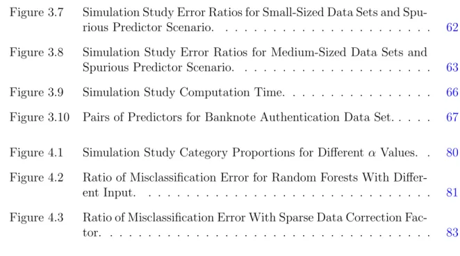
task is to predict the doppler function from these data with minimum squared error loss. Performance is evaluated at the 5000 points x∗i = i/5000. A plot of this function with the test case data is shown in Figure2.1.
● ● ● ● ● ● ● ● ● ● ● ● ● ● ● ● ● ● ● ● ●● ● ● ● ●● ● ● ● ● ● ● ● ● ● ● ● ● ● ● ● ● ● ● ● ● ● ● ● ● ● ● ● ● ● ● ● ● ● ● ● ● ● ● ● ● ● ● ● ● ● ● ● ● ● ●● ● ● ● ● ● ● ● ● ● ● ● ● ● ● ● ● ● ● ● ● ● ● ● ● ● ● ● ● ● ● ● ● ● ● ● ● ● ● ● ● ● ● ● ● ● ● ● ● ● ● ● ● ● ● ● ● ● ● ● ● ● ● ● ● ● ● ● ● ● ● ●● ● ● ● ● ● ● ● ● ● ● ● ● ● ● ● ● ● ● ●● ● ● ● ● ● ● ● ● ● ● ● ● ● ● ● ● ● ● ● ● ● ● ● ● ●● ● ● ● ● ● ● ● ● ● ● ● ● ● ● ● ● ● ● ● ● ● ● ● ● ● ● ● ● ● ● ● ● ● ● ● ● ● ● ● ● ● ● ● ● ● ● ● ● ● ● ● ● ● ● ●● ● ● ● ● ● ● ● ● ● ●● ● ● ● ● ● ● ● ● ● ● ● ● ● ● ● ● ● ● ● ● ● ● ● ● ● ● ● ● ●● ● ● ● ● ● ● ● ● ● ● ● ● ● ● ● ● ● ● ● ● ● ● ● ● ● ● ● ● ● ● ● ● ● ● ● ● ● ● ● ● ● ● ● ● ● ● ● ● ● ● ● ● ● ● ● ● ● ● ● ● ● ● ● ● ● ● ● ● ● ● ● ● ● ● ● ● ● ● ● ● ● ● ● ● ● ● ● ● ● ● ● ● ● ● ● ● ● ● ● ● ● ● ● ● ● ● ● ● ● ● ● ●●●● ● ● ● ● ● ● ● ● ● ● ● ● ● ● ● ● ● ● ● ● ● ● ● ● ● ● ● ● ● ● ● ● ● ● ● ● ● ● ● ● ● ● ● ● ● ● ● ● ● ● ● ● ● ● ● ● ● ● ● ● ● ● ● ● ● ● ● ● ●● ● ● ● ● ● ● ● ● ● ● ● ● ● ● ● ● ● ● ● ● ● ● ● ● ● ● ● ● ● ● ● ● ● ● ● ● ● ● ● ● ● ● ● ● ● ● ● ● ● ● ● ● ● ● ● ● ● ● ● ● ● ● ● ● ● ● ● ● ● ● ● ● ● ● ● ● ● ● ● ● ●● ● ● ● ●● ● ● ● ● ● ● ● ● ● ● ● ● ● ● ● ● ● ● ● ● ● ● ● ● ● ● ● ● ● ● ● ● ● ● ● ● ● ● ● ● ● ● ● ● ●●● ● ● ● ● ● ● ● ●● ● ● ● ● ● ● ● ● ● ● ● ● ● ● ● ● ● ● ● ● ● ● ● ● ● ● ● ● ● ● ● ● ● ● ● ● ● ● ● ● ● ● ● ● ● ● ● ● ● ● ● ● ● ● ● ● ● ● ● ● ● ● ● ● ● ● ● ● ● ● ● ● ● ● ● ● ● ● ● ● ● ● ● ● ● ● ● ● ● ● ● ● ● ● ● ● ● ● ● ● ● ● ● ● ● ● ● ● ● ● ● ●● ● ● ● ● ● ● ● ● ● ● ● ● ● ● ● ● ● ● ● ● ● ● ● ● ● ● ● ● ● ● ● ● ● ● ● ● ● ● ● ● ● ● ● ● ● ● ● ● ● ● ● ● ● ● ● ● ● ● ● ● ● ● ● ● ● ● ● ● ● ● ● ● ● ● ● ● ● ● ● ● ● ● ● ● ● ● ● ● ● ● ●● ● ● ● ● ● ● ● ● ● ● ● ● ● ● ● ● ● ● ● ● ● ● ● ● ●● ● ● ● ●●● ● ● ●● ● ● ● ● ● ● ● ● ● ● ● ● ● ● ● ● ● ● ● ● ● ● ● ● ● ● ● ● ● ● ● ● ● ● ● ● ● ● ● ●● ● ● ● ● ● ● ● ● ● ● ● ● ● ● ● ● ● ● ● ● ● ● ● ● ● ● ● ● ● ● ● ● ● ● ● ● ● ● ● ● ● ● ● ● ● ● ● ● ● ● ● ● ● ● ● ● ● ● ● ● ● ● ● ● ● ● ● ● ● ● ● ● ● ● ● ● ● ● ● ● ● ● ● ● ● ● ● ● ● ● ● ● ● ● ● ● ● ● ● ● ● ● ● ● ● ● ● ● ● ● ● ● ● ● ● ● ● ● ● ● ● ● ● ● ● ● ● ● ● ● ● ● ● ● ● ● ● ● ● ● ● ● ● ● ● ● ● ●● ● ● ● ● ● ● ● ● ● ● ● ● ● ● ● ● ● ● ● ● ● ● ● ● ● ● ● ● ● ● ● ● ● ● ● ● ● ● ● ● ● ● ● ● ● ● ● ● ● ● ● ● ● ● ●● ● ● ● ● ● ● ● ● ● ● ● ● ● ● ●● ● ● ● ● ● ● ● ● ● ● ● ● ● ● ● ● ● ● ● ● ● ● ● ● ● ● ● ● ● ● ● ● ● ● ● ● ● ● ● ● ● ● ● ● ● ● ● ● ● ● ● ● ● ● ● ● ● ● ● ● ● ● ● ● ● ● ● ● ● ● ● ● ● ● ● ● ● ● ● ● ● ● ● ● ● ● ● ● ● ● ● ● ● ● ● ● ● ● ● ● ●● ● ● ● ● ● ● ● ● ● ● ● ● ● ● ● ● ● ● ● ● ● ● ● ● ● ● ● ● ● ● ● ● ● ● ● ● ● ● ● ● ● ● ● ● ● ● ● ● ● ● ● ● ● ● ● ● ● ● ● ● ● ● ● ● ● ● ● ● ● ● ● ● ● ● ● ● ● ● ● ● ● ● ● ● ● ● ● ● ● ● ● ● ● ● ● ● ● ● ● ● ● ● ● ● ● ● ● ● ● ● ● ● ● ● ● ● ● ● ● ● ● ● ● ● ● ● ● ● ● ● ● ● ● ● ● ● ● ● ● ● ● ● ● ● ● ● ● ● ● ● ● ● ● ● ● ● ● ● ● ● ● ● ● ● ● ● ● ● ● ● ● ● ● ● ● ● ● ● ● ● ● ● ● ● ● ● ● ● ● ● ● ● ● ● ● ● ● ● ● ● ● ● ● ● ● ● ● ● ● ● ● ● ● ● ● ● ● ● ● ● ● ● ● ● ● ● ● ● ● ● ● ● ● ● ● ● ● ● ● ● ● ● ● ● ● ● ● ● ● ● ● ● ● ● ●● ● ● ● ● ● ● ● ● ● ●● ● ● ● ● ● ● ● ● ● ● ● ● ● ● ● ● ● ● ● ● ● ● ● ● ● ● ● ● ● ● ● ● ● ● ● ● ● ● ● ● ● ● ● ● ● ● ● ● ● ● ● ● ● ● ● ● ● ● ● ● ● ● ● ● ● ● ● ● ● ● ● ● ● ● ● ● ● ● ● ● ● ● ● ● ● ● ● ● ● ● ● ● ● ● ● ● ● ● ● ● ● ● ● ● ● ● ● ● ● ● ● ● ● ● ● ● ● ● ● ● ● ● ● ● ● ● ● ● ● ● ● ● ● ● ● ● ● ● ● ● ● ● ● ● ● ● ● ● ● ● ● ● ● ● ● ● ● ● ● ● ● ● ● ● ● ● ● ● ● ● ● ● ●● ● ● ● ● ● ● ● ● ● ● ● ● ● ● ● ● ● ● ● ● ● ● ● ● ● ● ● ● ● ●● ● ● ● ● ● ● ● ● ● ● ● ● ● ● ● ● ● ● ● ● ● ● ● ● ● ● ● ● ● ● ● ● ● ● ● ● ● ● ● ● ● ● ● ● ● ● ● ● ● ● ● ● ● ● ● ● ● ● ● ● ● ● ● ● ● ● ● ● ● ● ● ● ● ● ● ● ● ● ● ● ● ● ● ● ● ● ● ● ● ● ● ● ● ● ● ● ● ● ● ● ● ● ● ● ● ● ● ● ● ● ● ● ● ● ● ● ● ● ● ● ● ● ● ● ● ● ● ● ● ● ● ●● ● ● ● ● ● ● ● ● ● ● ● ● ● ●● ● ● ● ● ● ● ● ● ● ● ● ● ● ● ●● ● ● ● ●● ● ● ● ●● ● ● ● ● ● ● ● ● ●● ● ● ● ● ● ● ● ● ● ● ● ● ● ● ● ● ● ● ● ● ● ● ● ● ● ● ● ● ● ● ● ● ● ● ● ● ● ● ● ●● ● ● ● ● ● ● ● ● ● ● ● ● ● ● ● ● ● ● ● ● ● ● ● ● ● ● ● ● ● ● ● ● ● ● ● ● ● ● ● ● ● ● ● ● ● ● ● ● ● ● ● ● ● ● ● ● ● ● ● ● ●● ● ● ● ● ● ● ● ● ● ● ● ● ● ● ● ● ● ● ● ● ● ● ● ● ● ● ● ● ● ● ● ● ● ● ● ● ● ● ● ● ● ● ● ● ● ● ● ● ● ● ● ● ● ● ● ● ● ● ● ● ● ● ● 0.0 0.2 0.4 0.6 0.8 1.0 −1.0 −0.5 0.0 0.5 1.0 x y
Figure 2.1 Doppler Function Test Case Data. 2048 points from the doppler function (shown as line) with added error N(0,0.22).
We use the mixture prior Bayesian method to get predictions for the regression func-tion ofywith n= 30 latent mixture components and 171 scale matrices for the prior for Σm. The added Gaussian noise is regenerated to make 50 different test cases. In these
test cases the performance metric, sq. err., is the ratio of the sum of squared prediction errors compared with the true regression function f(xi) for observationsi= 1, . . . , Ntest, PNtest
i=1 (f(xi) −yˆi)2, relative to the total sum of squares for the regression function, PNtest
i=1 (f(xi)−E(yi))2. This error metric is proportional to the amount of unexplained
variation of the true regression function at the test data observations.
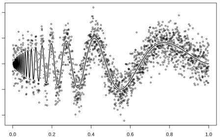
Figure 2.2 shows the prediction curves for Gaussian noise generated with the first random seed. The squared error ratio for this first seed are 0.0404 for local regression and 0.0616 for the mixture prior Bayesian method. Note that the small optimal bandwidth for the local regression method is chosen due to the variability at smallx values, leading to choppy predicted values for larger x. An appealing aspect of the mixture prior Bayesian method is its ability to adapt the smoothing bandwidth to the local regression function structure.
0.0 0.2 0.4 0.6 0.8 1.0 −0.6 −0.4 −0.2 0.0 0.2 0.4 0.6 x predicted v alue local regression mixture prior Bayes
Figure 2.2 Comparison of Doppler Function Prediction Values. Prediction curves based on local regression and mixture prior Bayes. Note that the mixture prior Bayesian method provides a smoother fit of the doppler function.
Table 2.1 Unexplained Variation of the Doppler Function for 50 Random Seeds
prediction method sq. err. mean sq. err. s.d. mixture prior Bayes 0.069 0.007 k-nearest neighbors (¯k = 18.6) 0.042 0.004 local linear regression 0.038 0.003
Table 2.1 shows results of prediction of the doppler functiond(x) over the same 5000 test points but with 50 different sets of random errors generated for the 2048 training data points. While prediction values for the mixture prior Bayesian method have higher squared error than other local regression methods such as k-nearest neighbors using R package FNN and local regression using R package locfit, the mixture prior Bayesian performance is not poor and this method does not overfit the data.
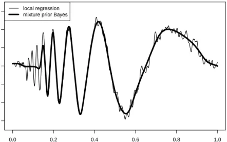
2.3.1.2 Performance with a spurious predictor
Prediction performance of the mixture prior Bayesian method improves over other local regression methods when the system has a spurious predictor, i.e., a variable
unre-lated to the response. A predictorX2 ∼Unif(0,1) is added to the previous test case, and prediction values are recalculated. Table 2.2 shows results of prediction of the doppler function d(x) values over the same 50 test cases as before, except now with a spurious second covariate generated from a uniform density. In this situation, performance of the mixture prior Bayesian method is substantially better than that of the local methods. It is interesting that the mixture prior Bayesian method has higher variability of unex-plained error even though its average error rate is much lower than that of the other two methods. Note that the average optimal number of neighbors in k-nearest neighbors is much lower in the presence of a spurious predictor.
Table 2.2 Unexplained Variation of the Doppler Function With Spurious Predictor for 50 Random Seeds
prediction method sq. err. mean sq. err. s.d. mixture prior Bayes 0.129 0.015 k-nearest neighbors (¯k = 7.7) 0.283 0.009 local linear regression 0.248 0.009
2.3.1.3 Performance with varying mixture prior input
The performance of the mixture prior Bayesian method changes greatly with the number of input scale matrices for Σm. Simply reducing the number of scale matrices
in-put into the mixture prior Bayesian method does not exactly mimic a standard Bayesian mixture model implementation. However, inputing only a single diffuse scale matrix in the mixture prior Bayesian method would result in a marginal prior for the mean and variance parameters that is approximately as diffuse as the marginal prior for a standard Bayesian mixture model. Therefore, the resulting performance degradation that occurs when using only diffuse scale matrices highlights the difficulties of the standard Bayes model mentioned in the introduction.
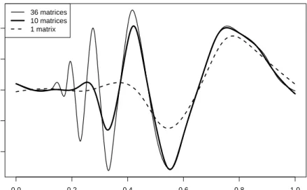
0.0 0.2 0.4 0.6 0.8 1.0 −0.4 −0.2 0.0 0.2 0.4 x predicted v alue 36 matrices 10 matrices 1 matrix
Figure 2.3 Fewer Scale Matrices Degrades Prediction Performance. The amount of empirical information provided to the Σm prior is reduced by decreasing the
maximum number of grouping in the clustering program. A less-informative prior leads to over-smoothed prediction values.
The same 50 test cases from 2.3.1.1 are rerun with varying empirical information provided to the Σm prior of the Bayes model. We reduce the number of scale matrices
by decreasing the maximum number of groupings found by the clustering algorithm. Ta-ble 2.3 shows prediction results with varying number of clustering algorithm cumulative groupings for the 50 test cases. The prediction curves for the first seed, shown in Fig-ure 2.3, demonstrate what typically happens: as less empirical information is provided to the Bayes model, the resulting more diffuse prior muddles the mixture arrangement in the posterior, leading to degraded prediction performance.
Table 2.3 Unexplained Variation of the Doppler Function With Various Scale Matrices Provided for Mixture Prior for 50 Random Seeds
no. of scale matrices 1 3 10 21 36 78 171 sq. err. mean .545 .285 .217 .137 .117 .086 .069 sq. err. s.d. .010 .009 .032 .016 .014 .010 .007
● ● ● ● ● ● ● ● ● ● ● ● ● ● ● ● ● ● ● ● ● ● ● ● ● ● ● ● ● ● ● ● ● ● ● ● ● ● ● ● ● ● ● ● ● ● ● ● ● ● ● ● ● ● ● ● ● ● ● ● ● ● ● ● ● ● ● ● ● ● ● ● ● ● ● ● ● ● ● ● ● ● ● ● ● ● ● ● ● ● ● ● ● ● ●● ● ● ● ● ● ● ● ● ● ● ● ● ● ● ● ● ● ● ● ● ● ● ● ● ● ● ● ● ● ● ● ● ● ● ● ● ● ● ● ● ● ● ● ● ● ● ● ● ● ● ● ● ● ● ● ● ● ● ● ● ● ● ● ● ● ● ● ● ● ● ● ● ● ● ● ● ● ● ● ● ● ● ● ● ● ● ● ● ● ● ● ● ● ● ● ● ● ● ● ● ● ● ● ● ● ● ● ● ● ● ● ● ● ● ● ● ● ● ● ● ● ● ● ● ● ● ● ● ● ● ● ● ● ● ● ● ● ● ● ● ● ● ● ● ● ● ● ● ● ● ● ● ● ● ● ● ● ● ● ● ● ● ● ● ● ● ● ● ● ● ● ● ● ● ● ● ● ● ● ● ● ● ● ● ● ● ● ● ● ● ● ● ● ● ● ● ● ● ● ● ● ● ● ● ● ● ● ● ● ● ● ● ● ● ● ● ● ● ● ● ● ● ● ●● ● ● ● ● ● ● ● ● ● ● ● ● ● ● ● ● ● ● ●● ● ● ● ● ● ● ● ● ● ● ● ● ● ● ● ● ● ● ● ● ● ● ● ● ● ● ● ● ● ● ● ● ● ● ● ● ● ● ● ● ● ● ● ● ● ● ● ● ● ● ● ● ● ● ● ● ● ● ● ● ● ● ● ● ● ● ● ● ● ● ● ● ● ● ● ● ● ● ● ● ● ● ● ● ● ● ● ● ● ● ● ● ● ● ● ● ● ● ● ● ● ● ● ● ● ● ● ● ● ● ● ● ● ● ● ● ● ● ● ● ● ● ● ● ● ● ● ● ● ● ● ● ● ● ● ● ● ● ● ● ● ● ● ● ● ● ● ● ● ● ● ● ● ● ● ● ● ● ● ● ● ● ● ● ● ● ● ● ● ● ● iteration #1 train[idsamp, 2] ● ● ● ● ● ● ● ● ● ● ● ● ● ● ● ● ● ● ● ● ● ● ● ● ● ● ● ● ● ● ● ● ● ● ● ● ● ● ● ● ● ● ● ● ● ● ● ● ● ● ● ● ● ● ● ● ● ● ● ● ● ● ● ● ● ● ● ● ● ● ● ● ● ● ● ● ● ● ● ● ● ● ● ● ● ● ● ● ● ● ● ● ● ● ●● ● ● ● ● ● ● ● ● ● ● ● ● ● ● ● ● ● ● ● ● ● ● ● ● ● ● ● ● ● ● ● ● ● ● ● ● ● ● ● ● ● ● ● ● ● ● ● ● ● ● ● ● ● ● ● ● ● ● ● ● ● ● ● ● ● ● ● ● ● ● ● ● ● ● ● ● ● ● ● ● ● ● ● ● ● ● ● ● ● ● ● ● ● ● ● ● ● ● ● ● ● ● ● ● ● ● ● ● ● ● ● ● ● ● ● ● ● ● ● ● ● ● ● ● ● ● ● ● ● ● ● ● ● ● ● ● ● ● ● ● ● ● ● ● ● ● ● ● ● ● ● ● ● ● ● ● ● ● ● ● ● ● ● ● ● ● ● ● ● ● ● ● ● ● ● ● ● ● ● ● ● ● ● ● ● ● ● ● ● ● ● ● ● ● ● ● ● ● ● ● ● ● ● ● ● ● ● ● ● ● ● ● ● ● ● ● ● ● ● ● ● ● ● ●● ● ● ● ● ● ● ● ● ● ● ● ● ● ● ● ● ● ● ●● ● ● ● ● ● ● ● ● ● ● ● ● ● ● ● ● ● ● ● ● ● ● ● ● ● ● ● ● ● ● ● ● ● ● ● ● ● ● ● ● ● ● ● ● ● ● ● ● ● ● ● ● ● ● ● ● ● ● ● ● ● ● ● ● ● ● ● ● ● ● ● ● ● ● ● ● ● ● ● ● ● ● ● ● ● ● ● ● ● ● ● ● ● ● ● ● ● ● ● ● ● ● ● ● ● ● ● ● ● ● ● ● ● ● ● ● ● ● ● ● ● ● ● ● ● ● ● ● ● ● ● ● ● ● ● ● ● ● ● ● ● ● ● ● ● ● ● ● ● ● ● ● ● ● ● ● ● ● ● ● ● ● ● ● ● ● ● ● ● ● ● iteration #10 train[idsamp, 2] tr ain[idsamp , 1] ● ● ● ● ● ● ● ● ● ● ● ● ● ● ● ● ● ● ● ● ● ● ● ● ● ● ● ● ● ● ● ● ● ● ● ● ● ● ● ● ● ● ● ● ● ● ● ● ● ● ● ● ● ● ● ● ● ● ● ● ● ● ● ● ● ● ● ● ● ● ● ● ● ● ● ● ● ● ● ● ● ● ● ● ● ● ● ● ● ● ● ● ● ● ●● ● ● ● ● ● ● ● ● ● ● ● ● ● ● ● ● ● ● ● ● ● ● ● ● ● ● ● ● ● ● ● ● ● ● ● ● ● ● ● ● ● ● ● ● ● ● ● ● ● ● ● ● ● ● ● ● ● ● ● ● ● ● ● ● ● ● ● ● ● ● ● ● ● ● ● ● ● ● ● ● ● ● ● ● ● ● ● ● ● ● ● ● ● ● ● ● ● ● ● ● ● ● ● ● ● ● ● ● ● ● ● ● ● ● ● ● ● ● ● ● ● ● ● ● ● ● ● ● ● ● ● ● ● ● ● ● ● ● ● ● ● ● ● ● ● ● ● ● ● ● ● ● ● ● ● ● ● ● ● ● ● ● ● ● ● ● ● ● ● ● ● ● ● ● ● ● ● ● ● ● ● ● ● ● ● ● ● ● ● ● ● ● ● ● ● ● ● ● ● ● ● ● ● ● ● ● ● ● ● ● ● ● ● ● ● ● ● ● ● ● ● ● ● ●● ● ● ● ● ● ● ● ● ● ● ● ● ● ● ● ● ● ● ●● ● ● ● ● ● ● ● ● ● ● ● ● ● ● ● ● ● ● ● ● ● ● ● ● ● ● ● ● ● ● ● ● ● ● ● ● ● ● ● ● ● ● ● ● ● ● ● ● ● ● ● ● ● ● ● ● ● ● ● ● ● ● ● ● ● ● ● ● ● ● ● ● ● ● ● ● ● ● ● ● ● ● ● ● ● ● ● ● ● ● ● ● ● ● ● ● ● ● ● ● ● ● ● ● ● ● ● ● ● ● ● ● ● ● ● ● ● ● ● ● ● ● ● ● ● ● ● ● ● ● ● ● ● ● ● ● ● ● ● ● ● ● ● ● ● ● ● ● ● ● ● ● ● ● ● ● ● ● ● ● ● ● ● ● ● ● ● ● ● ● ● iteration #100 train[idsamp, 2] tr ain[idsamp , 1] ● ● ● ● ● ● ● ● ● ● ● ● ● ● ● ● ● ● ● ● ● ● ● ● ● ● ● ● ● ● ● ● ● ● ● ● ● ● ● ● ● ● ● ● ● ● ● ● ● ● ● ● ● ● ● ● ● ● ● ● ● ● ● ● ● ● ● ● ● ● ● ● ● ● ● ● ● ● ● ● ● ● ● ● ● ● ● ● ● ● ● ● ● ● ●● ● ● ● ● ● ● ● ● ● ● ● ● ● ● ● ● ● ● ● ● ● ● ● ● ● ● ● ● ● ● ● ● ● ● ● ● ● ● ● ● ● ● ● ● ● ● ● ● ● ● ● ● ● ● ● ● ● ● ● ● ● ● ● ● ● ● ● ● ● ● ● ● ● ● ● ● ● ● ● ● ● ● ● ● ● ● ● ● ● ● ● ● ● ● ● ● ● ● ● ● ● ● ● ● ● ● ● ● ● ● ● ● ● ● ● ● ● ● ● ● ● ● ● ● ● ● ● ● ● ● ● ● ● ● ●● ● ● ● ● ● ● ● ● ● ● ● ● ● ● ● ● ● ● ● ● ● ● ● ● ● ● ● ● ● ● ● ● ● ● ● ● ● ● ● ● ● ● ● ● ● ● ● ● ● ● ● ● ● ● ● ● ● ● ● ● ● ● ● ● ● ● ● ● ● ● ● ● ● ● ● ● ● ● ● ● ● ● ● ● ● ● ● ●● ● ● ● ● ● ● ● ● ● ● ● ● ● ● ● ● ● ● ●● ● ● ● ● ● ● ● ● ● ● ● ● ● ● ● ● ● ● ● ● ● ● ● ● ● ● ● ● ● ● ● ● ● ● ● ● ● ● ● ● ● ● ● ● ● ● ● ● ● ● ● ● ● ● ● ● ● ● ● ● ● ● ● ● ● ● ● ● ● ● ● ● ● ● ● ● ● ● ● ● ● ● ● ● ● ● ● ● ● ● ● ● ● ● ● ● ● ● ● ● ● ● ● ● ● ● ● ● ● ● ● ● ● ● ● ● ● ● ● ● ● ● ● ● ● ● ● ● ● ● ● ● ● ● ● ● ● ● ● ● ● ● ● ● ● ● ● ● ● ● ● ● ● ● ● ● ● ● ● ● ● ● ● ● ● ● ● ● ● ● ● iteration #1 train[idsamp, 2] ● ● ● ● ● ● ● ● ● ● ● ● ● ● ● ● ● ● ● ● ● ● ● ● ● ● ● ● ● ● ● ● ● ● ● ● ● ● ● ● ● ● ● ● ● ● ● ● ● ● ● ● ● ● ● ● ● ● ● ● ● ● ● ● ● ● ● ● ● ● ● ● ● ● ● ● ● ● ● ● ● ● ● ● ● ● ● ● ● ● ● ● ● ● ●● ● ● ● ● ● ● ● ● ● ● ● ● ● ● ● ● ● ● ● ● ● ● ● ● ● ● ● ● ● ● ● ● ● ● ● ● ● ● ● ● ● ● ● ● ● ● ● ● ● ● ● ● ● ● ● ● ● ● ● ● ● ● ● ● ● ● ● ● ● ● ● ● ● ● ● ● ● ● ● ● ● ● ● ● ● ● ● ● ● ● ● ● ● ● ● ● ● ● ● ● ● ● ● ● ● ● ● ● ● ● ● ● ● ● ● ● ● ● ● ● ● ● ● ● ● ● ● ● ● ● ● ● ● ● ● ● ● ● ● ● ● ● ● ● ● ● ● ● ● ● ● ● ● ● ● ● ● ● ● ● ● ● ● ● ● ● ● ● ● ● ● ● ● ● ● ● ● ● ● ● ● ● ● ● ● ● ● ● ● ● ● ● ● ● ● ● ● ● ● ● ● ● ● ● ● ● ● ● ● ● ● ● ● ● ● ● ● ● ● ● ● ● ● ●● ● ● ● ● ● ● ● ● ● ● ● ● ● ● ● ● ● ● ●● ● ● ● ● ● ● ● ● ● ● ● ● ● ● ● ● ● ● ● ● ● ● ● ● ● ● ● ● ● ● ● ● ● ● ● ● ● ● ● ● ● ● ● ● ● ● ● ● ● ● ● ● ● ● ● ● ● ● ● ● ● ● ● ● ● ● ● ● ● ● ● ● ● ● ● ● ● ● ● ● ● ● ● ● ● ● ● ● ● ● ● ● ● ● ● ● ● ● ● ● ● ● ● ● ● ● ● ● ● ● ● ● ● ● ● ● ● ● ● ● ● ● ● ● ● ● ● ● ● ● ● ● ● ● ● ● ● ● ● ● ● ● ● ● ● ● ● ● ● ● ● ● ● ● ● ● ● ● ● ● ● ● ● ● ● ● ● ● ● ● ● iteration #10 train[idsamp, 2] tr ain[idsamp , 1] ● ● ● ● ● ● ● ● ● ● ● ● ● ● ● ● ● ● ● ● ● ● ● ● ● ● ● ● ● ● ● ● ● ● ● ● ● ● ● ● ● ● ● ● ● ● ● ● ● ● ● ● ● ● ● ● ● ● ● ● ● ● ● ● ● ● ● ● ● ● ● ● ● ● ● ● ● ● ● ● ● ● ● ● ● ● ● ● ● ● ● ● ● ● ●● ● ● ● ● ● ● ● ● ● ● ● ● ● ● ● ● ● ● ● ● ● ● ● ● ● ● ● ● ● ● ● ● ● ● ● ● ● ● ● ● ● ● ● ● ● ● ● ● ● ● ● ● ● ● ● ● ● ● ● ● ● ● ● ● ● ● ● ● ● ● ● ● ● ● ● ● ● ● ● ● ● ● ● ● ● ● ● ● ● ● ● ● ● ● ● ● ● ● ● ● ● ● ● ● ● ● ● ● ● ● ● ● ● ● ● ● ● ● ● ● ● ● ● ● ● ● ● ● ● ● ● ● ● ● ● ● ● ● ● ● ● ● ● ● ● ● ● ● ● ● ● ● ● ● ● ● ● ● ● ● ● ● ● ● ● ● ● ● ● ● ● ● ● ● ● ● ● ● ● ● ● ● ● ● ● ● ● ● ● ● ● ● ● ● ● ● ● ● ● ● ● ● ● ● ● ● ● ● ● ● ● ● ● ● ● ● ● ● ● ● ● ● ● ●● ● ● ● ● ● ● ● ● ● ● ● ● ● ● ● ● ● ● ●● ● ● ● ● ● ● ● ● ● ● ● ● ● ● ● ● ● ● ● ● ● ● ● ● ● ● ● ● ● ● ● ● ● ● ● ● ● ● ● ● ● ● ● ● ● ● ● ● ● ● ● ● ● ● ● ● ● ● ● ● ● ● ● ● ● ● ● ● ● ● ● ● ● ● ● ● ● ● ● ● ● ● ● ● ● ● ● ● ● ● ● ● ● ● ● ● ● ● ● ● ● ● ● ● ● ● ● ● ● ● ● ● ● ● ● ● ● ● ● ● ● ● ● ● ● ● ● ● ● ● ● ● ● ● ● ● ● ● ● ● ● ● ● ● ● ● ● ● ● ● ● ● ● ● ● ● ● ● ● ● ● ● ● ● ● ● ● ● ● ● ● iteration #100 train[idsamp, 2] tr ain[idsamp , 1] ● ● ● ● ● ● ● ● ● ● ● ● ● ● ● ● ● ● ● ● ● ● ● ● ● ● ● ● ● ● ● ● ● ● ● ● ● ● ● ● ● ● ● ● ● ● ● ● ● ● ● ● ● ● ● ● ● ● ● ● ● ● ● ● ● ● ● ● ● ● ● ● ● ● ● ● ● ● ● ● ● ● ● ● ● ● ● ● ● ● ● ● ● ● ●● ● ● ● ● ● ● ● ● ● ● ● ● ● ● ● ● ● ● ● ● ● ● ● ● ● ● ● ● ● ● ● ● ● ● ● ● ● ● ● ● ● ● ● ● ● ● ● ● ● ● ● ● ● ● ● ● ● ● ● ● ● ● ● ● ● ● ● ● ● ● ● ● ● ● ● ● ● ● ● ● ● ● ● ● ● ● ● ● ● ● ● ● ● ● ● ● ● ● ● ● ● ● ● ● ● ● ● ● ● ● ● ● ● ● ● ● ● ● ● ● ● ● ● ● ● ● ● ● ● ● ● ● ● ● ●● ● ● ● ● ● ● ● ● ● ● ● ● ● ● ● ● ● ● ● ● ● ● ● ● ● ● ● ● ● ● ● ● ● ● ● ● ● ● ● ● ● ● ● ● ● ● ● ● ● ● ● ● ● ● ● ● ● ● ● ● ● ● ● ● ● ● ● ● ● ● ● ● ● ● ● ● ● ● ● ● ● ● ● ● ● ● ● ●● ● ● ● ● ● ● ● ● ● ● ● ● ● ● ● ● ● ● ●● ● ● ● ● ● ● ● ● ● ● ● ● ● ● ● ● ● ● ● ● ● ● ● ● ● ● ● ● ● ● ● ● ● ● ● ● ● ● ● ● ● ● ● ● ● ● ● ● ● ● ● ● ● ● ● ● ● ● ● ● ● ● ● ● ● ● ● ● ● ● ● ● ● ● ● ● ● ● ● ● ● ● ● ● ● ● ● ● ● ● ● ● ● ● ● ● ● ● ● ● ● ● ● ● ● ● ● ● ● ● ● ● ● ● ● ● ● ● ● ● ● ● ● ● ● ● ● ● ● ● ● ● ● ● ● ● ● ● ● ● ● ● ● ● ● ● ● ● ● ● ● ● ● ● ● ● ● ● ● ● ● ● ● ● ● ● ● ● ● ● ● iteration #1 ● ● ● ● ● ● ● ● ● ● ● ● ● ● ● ● ● ● ● ● ● ● ● ● ● ● ● ● ● ● ● ● ● ● ● ● ● ● ● ● ● ● ● ● ● ● ● ● ● ● ● ● ● ● ● ● ● ● ● ● ● ● ● ● ● ● ● ● ● ● ● ● ● ● ● ● ● ● ● ● ● ● ● ● ● ● ● ● ● ● ● ● ● ● ●● ● ● ● ● ● ● ● ● ● ● ● ● ● ● ● ● ● ● ● ● ● ● ● ● ● ● ● ● ● ● ● ● ● ● ● ● ● ● ● ● ● ● ● ● ● ● ● ● ● ● ● ● ● ● ● ● ● ● ● ● ● ● ● ● ● ● ● ● ● ● ● ● ● ● ● ● ● ● ● ● ● ● ● ● ● ● ● ● ● ● ● ● ● ● ● ● ● ● ● ● ● ● ● ● ● ● ● ● ● ● ● ● ● ● ● ● ● ● ● ● ● ● ● ● ● ● ● ● ● ● ● ● ● ● ● ● ● ● ● ● ● ● ● ● ● ● ● ● ● ● ● ● ● ● ● ● ● ● ● ● ● ● ● ● ● ● ● ● ● ● ● ● ● ● ● ● ● ● ● ● ● ● ● ● ● ● ● ● ● ● ● ● ● ● ● ● ● ● ● ● ● ● ● ● ● ● ● ● ● ● ● ● ● ● ● ● ● ● ● ● ● ● ● ●● ● ● ● ● ● ● ● ● ● ● ● ● ● ● ● ● ● ● ●● ● ● ● ● ● ● ● ● ● ● ● ● ● ● ● ● ● ● ● ● ● ● ● ● ● ● ● ● ● ● ● ● ● ● ● ● ● ● ● ● ● ● ● ● ● ● ● ● ● ● ● ● ● ● ● ● ● ● ● ● ● ● ● ● ● ● ● ● ● ● ● ● ● ● ● ● ● ● ● ● ● ● ● ● ● ● ● ● ● ● ● ● ● ● ● ● ● ● ● ● ● ● ● ● ● ● ● ● ● ● ● ● ● ● ● ● ● ● ● ● ● ● ● ● ● ● ● ● ● ● ● ● ● ● ● ● ● ● ● ● ● ● ● ● ● ● ● ● ● ● ● ● ● ● ● ● ● ● ● ● ● ● ● ● ● ● ● ● ● ● ● iteration #10 tr ain[idsamp , 1] ● ● ● ● ● ● ● ● ● ● ● ● ● ● ● ● ● ● ● ● ● ● ● ● ● ● ● ● ● ● ● ● ● ● ● ● ● ● ● ● ● ● ● ● ● ● ● ● ● ● ● ● ● ● ● ● ● ● ● ● ● ● ● ● ● ● ● ● ● ● ● ● ● ● ● ● ● ● ● ● ● ● ● ● ● ● ● ● ● ● ● ● ● ● ●● ● ● ● ● ● ● ● ● ● ● ● ● ● ● ● ● ● ● ● ● ● ● ● ● ● ● ● ● ● ● ● ● ● ● ● ● ● ● ● ● ● ● ● ● ● ● ● ● ● ● ● ● ● ● ● ● ● ● ● ● ● ● ● ● ● ● ● ● ● ● ● ● ● ● ● ● ● ● ● ● ● ● ● ● ● ● ● ● ● ● ● ● ● ● ● ● ● ● ● ● ● ● ● ● ● ● ● ● ● ● ● ● ● ● ● ● ● ● ● ● ● ● ● ● ● ● ● ● ● ● ● ● ● ● ● ● ● ● ● ● ● ● ● ● ● ● ● ● ● ● ● ● ● ● ● ● ● ● ● ● ● ● ● ● ● ● ● ● ● ● ● ● ● ● ● ● ● ● ● ● ● ● ● ● ● ● ● ● ● ● ● ● ● ● ● ● ● ● ● ● ● ● ● ● ● ● ● ● ● ● ● ● ● ● ● ● ● ● ● ● ● ● ● ●● ● ● ● ● ● ● ● ● ● ● ● ● ● ● ● ● ● ● ●● ● ● ● ● ● ● ● ● ● ● ● ● ● ● ● ● ● ● ● ● ● ● ● ● ● ● ● ● ● ● ● ● ● ● ● ● ● ● ● ● ● ● ● ● ● ● ● ● ● ● ● ● ● ● ● ● ● ● ● ● ● ● ● ● ● ● ● ● ● ● ● ● ● ● ● ● ● ● ● ● ● ● ● ● ● ● ● ● ● ● ● ● ● ● ● ● ● ● ● ● ● ● ● ● ● ● ● ● ● ● ● ● ● ● ● ● ● ● ● ● ● ● ● ● ● ● ● ● ● ● ● ● ● ● ● ● ● ● ● ● ● ● ● ● ● ● ● ● ● ● ● ● ● ● ● ● ● ● ● ● ● ● ● ● ● ● ● ● ● ● ● iteration #100 tr ain[idsamp , 1]
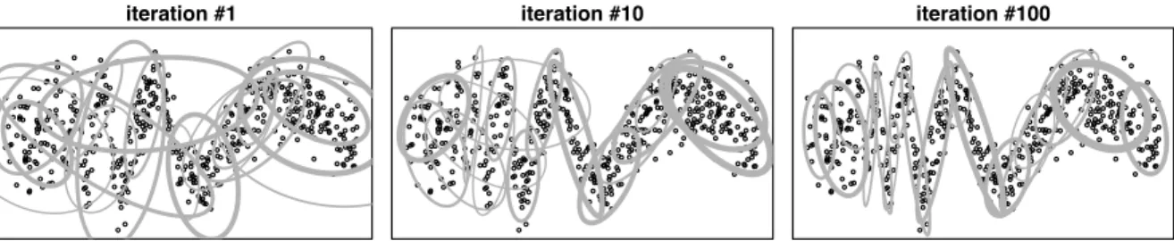
Figure 2.4 Component Parameters During Gibbs Sampler Initialization. 90% probabil-ity contours are shown forµm and Σm for any components with membership
more than 10 data points. Width of contour ellipse is relative to the com-ponent mixture proportion size.
The left panel of Figure2.4 shows 90% probability contours of the Gaussian parame-ters for the 24 latent mixture component parameparame-ters as the Gibbs sampler starts up. In this simulation, 171 scale matrices are provided for the prior of Σm. While the population
mixture is not apparent in the initial Gibbs sampling of the posterior, the posterior dis-tribution largely has the structure of the regression function and this structure is present in the sampler by the 100th iteration, shown in the right panel of Figure 2.4.
2.3.2 Comprehensive simulation study
A comprehensive simulation study of higher-dimensional simulated data is presented to show how the method performs in a variety of mixture distribution situations. This simulation study is loosely modeled after the comprehensive nonparametric regression testing in Banks et al. (2003). A regression function is created, simulated data are generated, and predictions are made using this mixture prior Bayesian method and four comparison methods. Each scenario is randomly regenerated a total of 25 times and performance of each method is assessed using a prediction error ratio.
2.3.2.1 Generation of simulated test cases
The study focuses on prediction of a continuous response whose regression function is the conditional mean function of a mixture of eight multivariate normal densities
E(Y|X =x) = 8 X h=1 ph(x) µh,y+ Σh,yxΣ−h,xx1 (x−µh,x) (2.5)
where ph(x) is the probability that an observation at xis from density h. Note that the
eight probabilitiesph(x) sum to one for anyx, and these probabilities consider the density
population proportion sizes for the eight densities. ph(x) is equal to the component h
density evaluated at x times the component proportion size, and then these eightph(x)
values are rescaled so they sum to one.
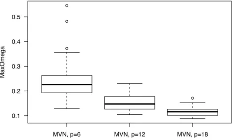
Simulations use multivariate normal component parameters generated from R package MixSim (Melnykov et al., 2012). The amount of overlap can be specified when generating data with MixSim, and we choose an average overlap of ¯ω = .05 for the simulations, which specifies low mixture component separation (Melnykov and Maitra, 2010). We also choose non-spherical densities and draw the first seven mixture proportions from Stick(α= 16, β = 64), with the eighth mixture assigned the remaining probability. After the Gaussian component parameters and mixture proportions are determined, data are generated with MixSim function simdataset using default choices for all other parameters. We use the MixSim package to calculate the amount of cluster overlap in our simulated data sets. Our implementation of MixSim has a single purpose, and that purpose is to get a locally linear conditional response function calculated by equation 2.5. MixSim provides mean and covariance values µh and Σh for the eight densities of our mixture
distribution. By altering the MixSim component proportions to match those from our stick-breaking proportion assignments, the average overlap ¯ω differs from the target of .05. Instead, the observed average overlap ranges from .052 to .062 in our test cases. The maximum overlap ˇω measures the highest level of overlap between the densities of the mixture. See Figure 2.5 for a plot showing calculated maximum overlap ˇω values
for the multivariate normal data generation scenario (see2.3.2.2 below) for the different number of predictors in the simulation study. As the dimension increases and the number of components stays fixed at eight densities, the probability that any two components exhibit high overlap decreases.
● ● ● MVN, p=6 MVN, p=12 MVN, p=18 0.052 0.054 0.056 0.058 0.060
calculated BarOmega values
BarOmega ● ● ● ● MVN, p=6 MVN, p=12 MVN, p=18 0.1 0.2 0.3 0.4 0.5
calculated MaxOmega values
MaxOmega 0.052 0.054 0.056 0.058 0.060 0.4 0.6 0.8 1.0
MVN−generated data from mixture of 8 densities
p=6, small(red), medium(blue), large(green)
BarOmega Mixture Pr ior − to − Lik elihood GMM error r atio ● ● ● ● ● ● ● ● ● ● ● ● ● ● ● ● ● ● ● ● ● ● ● ● ● ● ● ● ● ● ● ● ● ● ● ● ● ● ● ● ● ● ● ● ● ● ● ● ● ● ● ● ● ● ● ● ● ● ● ● ● ● ● ● ● ● ● ● ● ● ● ● ● ● ● 0.1 0.2 0.3 0.4 0.5 0.6 0.4 0.6 0.8 1.0
MVN−generated data from mixture of 8 densities
p=6, small(red), medium(blue), large(green)
MaxOmega Mixture Pr ior − to − Lik elihood GMM error r atio ● ● ● ● ● ● ● ● ● ● ● ● ● ● ● ● ● ● ● ● ● ● ● ● ● ● ● ● ● ● ● ● ● ● ● ● ● ● ● ● ● ● ● ● ● ● ● ● ● ● ● ● ● ● ● ● ● ● ● ● ● ● ● ● ● ● ● ● ● ● ● ● ● ● ●
Figure 2.5 Maximum Component Overlap From MixSim-Generated Data. These box-plots show the range of the maximum overlap (MaxOmega) values ˇω calcu-lated with the MixSim package function overlap. These values are calcucalcu-lated from all test cases of the multivariate normal data generation scenario, see
2.3.2.2. The three p values represent the number of predictors in the test cases.
2.3.2.2 Simulated test case scenarios
Testing is performed for three data dimensions (p= 6, 12, and 18 covariates), three data set sizes Nobs = k(1.2)p (k = 200, 500, 1250), and these three data generation
scenarios:
MVN Data. Data are generated from an eight-component multivariate Gaussian mix-ture. This scenario is an ideal situation for the mixture prior Bayesian prediction method and we expect the mixture prior Bayesian prediction method to perform well.
Uniform X. The regression function is generated from the eight-component multi-variate normal mixture, but then the predictors are regenerated from independent
Uni-form(0,1). The responseY equals the regression function atX =xplus N(0,0.12) noise. This scenario tests how the method performs when the multivariate normal structure in the predictors is lost and the only relationship available is the locally linear regression function. The mixture prior Bayesian method might not perform well in this case as all of the multivariate normal structure is gone except for the regression function.
Spurious. Data are generated from an eight-component multivariate Gaussian mixture as in the first scenario, except now one-third of the predictors are spurious with respect to, i.e. independent of, all other variables. This scenario tests how the methods are able to handle noisy predictors in the absence of variable selection.
2.3.2.3 Local regression methods for comparison
The method’s prediction performance, as measured in squared error relative to the true regression function given the predictors, is compared with the following four meth-ods.
Method G. The first comparison method is a likelihood-based Gaussian mixture method implemented via the MATLAB package gmdistribution using the function fitg-mdist. The likelihood-based method first requires determination of the optimal number of mixture components. This optimal number is found through 5-fold cross-validation, using a certain number of restarts that scales with the square root of the dimension. Once the optimal component number is determined, then many restarts are tried in the final model. See Figure 2.6 for quartiles of the optimal number of components densities in the Gaussian mixture model. At p= 18 predictors, the correct number of eight sub-populations is the optimal number of mixture components for each run. The variability of optimal components greatly increases for the uniform regeneration scenario.
Method B. The second comparison method is a diffuse prior Bayesian mixture model. Instead of independence of between the mean and covariance parameters, a conditional structure in the prior of a traditional Bayesian mixture model approach may yield better
● ● ● ● ● ● ● ●● ● ● ● ● ● ● ●● ● ● ● ● ● ●● ● ● ● 4 6 8 10 12
optimal number of components p=6 p=12 p=18 MVN data Uniform X Spurious
Figure 2.6 Optimal Number of Components for the Likelihood-Based Method. These are boxplots showing the determined number of components per run for the MATLAB implementation of Gaussian mixture models for prediction.
results. We implement in C a prediction method that uses the conditionally conjugate normal–inverse-Wishart prior of the classification mixture model given in Gelman et al. (2013). Good results came from using a scale matrix equal to one-half of the empirical covariance of the whole data, and that is the scale matrix used in the prior for Σm. All
other parameters are the same as the mixture prior Bayesian implementation.
Method N. The third comparison method is k-nearest neighbors implemented in R using library FNN function knn.reg. The optimalkneighbors is determined with 20-fold cross-validation by optimizing the internal calculation for leave-one-out cross-validation of function knn.reg. See Figure 2.7 for quartiles of the optimal number of neighbors for k-nearest neighbors. The uniform regenerated cases have lower optimal numbers of neighbors than the other data-generation scenarios. The variability of optimal k does not diminish as the dimension increases.
● ●
● ●
10 20 30 40 50 60
optimal number of neighbors p=6 p=12 p=18 MVN data Uniform X Spurious
Figure 2.7 Optimal Number of Neighbors for k-Nearest Neighbors. These are boxplots for the optimal number of neighbors determined by the R implementation of k-nearest neighbors for prediction.
Method F. The fourth comparison method is random forests implemented in R using library randomForest with default parameters. As overfitting is not a significant concern for random forests, the method is allowed to run for a long time until a stopping rule decides that enough trees have been grown to minimize prediction bias. The stopping rule is satisfied when linear regression on the out-of-bag prediction error for the previous 400 trees has a positive slope, meaning that the bias reduction has largely ceased.
Others. Other methods are not reported because they do not offer better results and are not be expected to predict a linear response well. Gradient boosting models (Hastie et al., 2009) and support vector regression do not have better results than the above methods. Multivariate adaptive regression splines and locally linear regression have computational difficulties with the dimension of these data sets; besides, both do not predict well for higher-dimensional data (Banks et al., 2003).
2.3.2.4 Simulated test case results
The comprehensive test case results are summarized in two plots, Figures2.8 and2.9. Figure 2.8 displays results across all scenarios, data set sizes, and dimensionality. Fig-ure 2.9 displays complete results for p= 6 covariates.
We determine the following findings about mixture prior Bayesian prediction perfor-mance from the simulation study results shown in Figure 2.8, grouped by comparison methods.
Likelihood-Based Methods. The mixture prior Bayesian method outperforms the like-lihood-maximizing solution across all scenarios as long as the dimension is not moderately large (p < 18) and the data set size is not large relative to the number of predictors p. This convergence of Bayesian and frequentist solutions as sample size increases is sensible because the prior distribution is dominated by the likelihood as the amount of data in-creases. It is reasonable that the Bayesian solution is slightly better, even with plentiful data, as the frequentist solution uses only one arrangement of mixture components while the Bayesian solution can average several equally good, though different, arrangements via the Dirichlet process prior. For 18 predictors, the data set size (Nobs = 13,312) is
large enough for the frequentist solution to perform similarly. This indicates that the chosen scale of 1.2 for the data size inflation formula, Nobs =k(1.2)p, may be too large.
We conjecture a constant of 1.1 might give more comparable results across dimension-ality. An alternative explanation is that the reduced maximum overlap values at higher dimensions leads to both easier prediction and similarity in results.