2011
Modular Algorithms for Biomolecular Network
Alignment
Fadi George Towfic
Iowa State UniversityFollow this and additional works at:
https://lib.dr.iastate.edu/etd
Part of the
Computer Sciences Commons
This Dissertation is brought to you for free and open access by the Iowa State University Capstones, Theses and Dissertations at Iowa State University Digital Repository. It has been accepted for inclusion in Graduate Theses and Dissertations by an authorized administrator of Iowa State University Digital Repository. For more information, please [email protected].
Recommended Citation
Towfic, Fadi George, "Modular Algorithms for Biomolecular Network Alignment" (2011).Graduate Theses and Dissertations. 12031. https://lib.dr.iastate.edu/etd/12031
by
Fadi George Towfic
A dissertation submitted to the graduate faculty in partial fulfillment of the requirements for the degree of
DOCTOR OF PHILOSOPHY
Major: Bioinformatics and Computational Biology
Program of Study Committee: Vasant Honavar, Co-major professor M. Heather West Greenlee, Co-major professor
Drena Dobbs Robert Jernigan Christopher Tuggle
Iowa State University Ames, Iowa
2011
DEDICATION
This dissertation is dedicated to my parents, for their endless support, constant encourage-ment and sage advice.
TABLE OF CONTENTS
LIST OF TABLES . . . vii
LIST OF FIGURES . . . x
ACKNOWLEDGEMENTS . . . xvii
ABSTRACT . . . .xviii
CHAPTER 1. INTRODUCTION . . . 1
1.1 Overview of network models and systems biology . . . 1
1.2 The network alignment problem . . . 3
1.3 Formal mathematical definition of network alignment . . . 5
1.4 Brief overview of state-of-the-art methods . . . 5
1.4.1 MaWISh . . . 5
1.4.2 NetworkBLAST-M . . . 6
1.4.3 Graemlin . . . 7
1.4.4 GRAAL . . . 8
1.5 Limitations of current methods . . . 8
1.6 Significant contributions of dissertation . . . 9
1.6.1 First highly modular algorithm in the field . . . 9
1.6.2 Highly scalable algorithm . . . 9
1.6.3 First highly flexible algorithm . . . 9
1.6.4 Highly portable . . . 10
1.6.5 High accuracy in terms of biological performance . . . 10
CHAPTER 2. BIOMOLECULAR NETWORK ALIGNMENT (BiNA)
TOOLKIT . . . 12
2.1 Background and Motivation . . . 13
2.2 Problem Formulation . . . 15
2.3 Algorithm . . . 16
2.3.1 Divide: Partitioning methods . . . 16
2.3.2 Conquer: Scoring Functions . . . 19
2.4 Summary and Discussion . . . 23
CHAPTER 3. COMPARATIVE ANALYSIS OF TOPOLOGICAL VS. NODE LABEL-BASED NETWORK ALIGNMENT . . . 26
3.1 Introduction . . . 26
3.2 Materials and methods . . . 29
3.2.1 Network Alignment Algorithm . . . 29
3.2.2 Scoring Functions . . . 32
3.2.3 Datasets . . . 36
3.2.4 Evaluation of Alignment . . . 37
3.3 Results . . . 38
3.3.1 Performance as Measured by GO Enrichment . . . 38
3.3.2 Reconstruction of Phylogenetic Relationships . . . 40
3.4 Discussion and conclusions . . . 43
CHAPTER 4. DETECTION OF GENE ORTHOLOGY FROM GENE CO-EXPRESSION AND PROTEIN INTERACTION NETWORKS . . . 47
4.1 Introduction . . . 48
4.2 Materials and methods . . . 50
4.2.1 Dataset . . . 50
4.2.2 Graph representation of BLAST orthologs . . . 51
4.2.3 Random walk graph kernel score . . . 52
4.2.5 Betweenness score . . . 54
4.2.6 Degree distribution score . . . 54
4.2.7 HITS score . . . 54
4.2.8 Scoring candidate orthologs based on sequence and network similarity . 55 4.2.9 Ortholog detection . . . 55
4.2.10 Performance evaluation . . . 56
4.3 Analysis and results . . . 57
4.3.1 Reconstructing KEGG orthologs using BLAST . . . 57
4.3.2 Reconstructing KEGG orthologs using sequence, protein-protein interac-tion network, and gene-coexpression data . . . 57
4.4 Discussion and future work . . . 58
CHAPTER 5. B CELL LIGAND GENE COEXPRESSION NETWORKS REVEAL REGULATORY PATHWAYS FOR LIGAND PROCESSING . 67 CHAPTER 6. TOOLS . . . 96
6.1 BiNA webserver . . . 96
6.2 BiNA program . . . 98
CHAPTER 7. CONCLUSIONS . . . 101
7.1 Significant contributions of dissertation . . . 102
7.1.1 First highly modular algorithm in the field . . . 102
7.1.2 Highly scalable algorithm . . . 102
7.1.3 First highly flexible algorithm . . . 102
7.1.4 Highly portable . . . 103
7.1.5 High accuracy in terms of biological performance . . . 103
7.1.6 Applied to important biological problems . . . 103
7.2 Open problems . . . 104
7.2.1 Evaluation methods . . . 104
7.2.2 Applicability to more network models . . . 104
7.2.4 Rapid comparisons . . . 105
7.2.5 Integrated pipeline for analysis and visualization . . . 106
APPENDIX. ADDITIONAL MATERIAL FOR CHAPTER 6 . . . 107
LIST OF TABLES
Table 3.1 Comparison of Graph Kernel Performance using BLAST to match initial node centers in K-Hop alignment between human (Hs), mouse (Mm), yeast (Sc) and fly (Dm). Bold entries are adapted from our previ-ous results on K-hop alignments (152). The methods are denoted as SP (Shortest Path), RW (Random Walk), PR (Page Rank), KL (Kull-back–Leibler divergence), Pearson (Pearson correlation), Spearman (Spear-man rank correlation) and Chi (Chi-squared test statistic). . . 41
Table 3.2 Comparison of Graph Kernel Performance using pure topological align-ment . . . 42
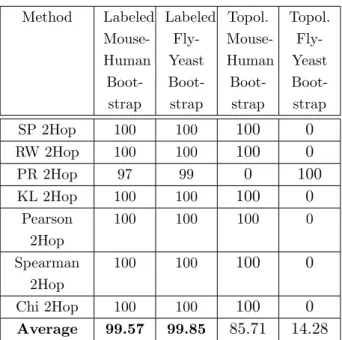
Table 3.3 Comparison of the bootstrap performance in reconstructing phyloge-netic relationships between mouse-human and fly-yeast branches . . . . 44
Table 4.1 Performance of the Reciprocal BLAST hit method on the fly, yeast, human and mouse protein-protein interaction datasets from DIP as well as the gene coexpression networks for mouse and human from GEO . . 60
Table 4.2 Performance of the Reciprocal BLAST hit score as a feature to the decision tree (j48), Naive Bayes (NB), Support Vector Machine (SVM) and Ensemble classifiers on the fly, yeast, human and mouse protein-protein interaction datasets from DIP as well as the gene coexpression networks for mouse and human from GEO. Values in parenthesis are the ranks for the classifiers on the specified dataset . . . 65
Table 4.3 Performance of all the combined features (Reciprocal BLAST hit score, 1 and 2 hop shortest path graph kernel score, 1 and 2 hop random walk graph kernel score, BaryCenter, betweenness, degree distribution and HITS) as input to the decision tree (j48), Naive Bayes (NB), Support Vector Machine (SVM) and Ensemble classifiers on the fly, yeast, human and mouse protein-protein interaction datasets from DIP as well as the gene coexpression networks for mouse and human from GEO. Values in parenthesis are the ranks for the classifiers on the specified dataset . . 65
Table 4.4 KEGG orthologs detected using the Ensemble classifier utilizing all net-work features. The orthologs shown in the above table were missed by the BLAST logistic regression classifier . . . 66
Table 5.1 Full list of the ligands and their abbreviations used in the experiments analyzed in this paper. This list was adapted from Lee et al. (104) . . 91
Table 5.2 List of pathways detected based on high-intensity probes from the mi-croarray data. Please see Table 1 in supplementary material for a more detailed version of this table with pathway names and relative number of genes enriched in the pathway based on the data . . . 92
Table 5.3 Top matched ligands based on expression patterns in the consensus tree shown in Figure 5. The KEGG pathway categories correspond to the pathway categories highlighted in Table 2. Please see Table 3 in the supplementary material for an expanded version of this table . . . 95
Table A.1 Full list of networks and the number of neighborhoods utilized for com-paring the networks for figure 2 in supplementary material. . . 110
Table A.2 List of pathways detected based on high-intensity probes from the mi-croarray data. As can be seen from the table, many of the pathways enriched in high-intensity genes are known to be implicated in the de-velopment of the immune system and processing of antigens . . . 118
Table A.3 Top matched ligands based on expression patterns in the consensus tree shown in figure 5 in the paper. The KEGG pathway categories corre-spond to the pathway categories highlighted in table 2 in the supple-mentary material and table 2 in the paper . . . 126
LIST OF FIGURES
Figure 1.1 Original figure from Koyuturk et al. (97). The Duplication/Elimination/Emergence model considered in MaWISh. Starting with three interactions between
three proteins, protein u1 is duplicated to add u1 into the network
to-gether with its interactions (dashed circle and lines). Then, u1 loses its
interaction with u3 (dotted line). Finally, an interaction between u1 and
u1 is added to the network (dashed line) . . . 6
Figure 1.2 Slightly modified figure from Kalaev et al. (81). A seed defined by a
d-identical-spine subnet (d = 3 in the above example since there are 3
k-spines), where the k-spines are restricted to be paths with identical topology. The dashed blue line encloses one of the three k-spines. The phylogenetic tree used to order the connection operation of the inter-layer edges of thek-spines is shown at the top of the figure . . . 11
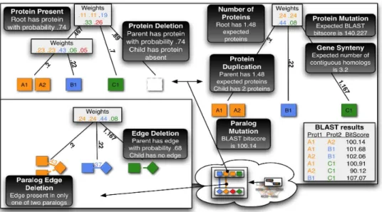
Figure 1.3 Original figure from Flannick et al. (56). This figure shows the set of evolutionary events that are computed by Graemlin’s node and edge feature functions. Graemlin 2.0 uses a phylogenetic tree with branch lengths to determine the events. First, the species weight vectors (shown as gray boxes) at each internal node of the tree are constructed; the weight vector represents the similarity of each extant species to the internal node. Graemlin 2.0 uses these weight vectors to compute the likely evolutionary events (shown as black boxes) that occur . . . 11
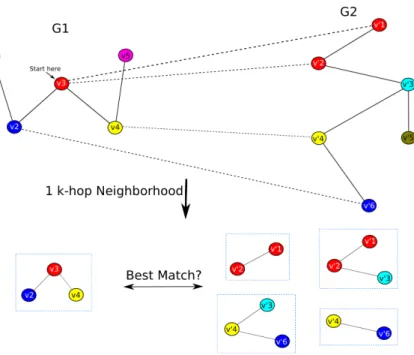
Figure 2.1 General schematic of thek-hop neighborhood alignment algorithm. The input to the algorithm are two graphs (G1 and G2) with corresponding
relationships among their nodes using mapping matrixP(similarly col-ored nodes are sequence homologous according to a BLAST search, for examplePv2v0
6 = 1). The algorithm starts at an arbitrary vertex in G1
(red vertex in the figure) and constructs a k-hop neighborhood around the starting vertex (1-hop neighborhood in the figure). The algorithm then matches each of the nodes in the 1-hop neighborhood subgraph from G1 to nodes in G2 using mapping matrix P. 1-hop subgraphs are
then constructed around each of the matching vertices. The 1-hop sub-graphs fromG2are then compared using a scoring function (e.g. a graph
kernel) to the 1-hop subgraph fromG1and the maximum scoring match
is returned. . . 17
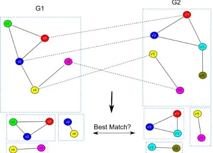
Figure 2.2 Schematic for the cluster-based alignment algorithm. The input to the algorithm are two graphs (G1 andG2) with corresponding relationships
among their nodes using mapping matrixP(similarly colored nodes are sequence homologous according to a BLAST search, for examplePv2v02 =
1). Subgraphs are generated fromG1 and G2 using a graph clustering
algorithm (e.g. bicomponent clusterer that finds biconnected subgraphs) and the subgraphs from G1 are compared against the subgraphs from G2 to find the best matching subgraphs using an appropriate scoring
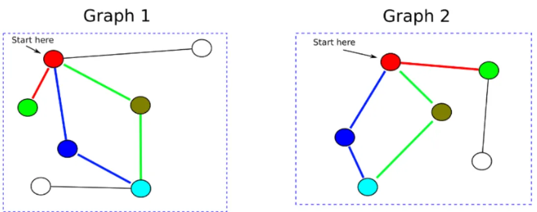
Figure 2.3 An example of the graph matching conducted by the shortest path graph kernel. Similarly colored nodes are sequence homologous according to a BLAST search. As can be seen from the figure, the graph kernel compares the lengths of the shortest paths around homologous vertices across the two graphs. The red edges show the matching shortest path in both graphs as computed by the graph kernel. The shortest path distance graph kernel takes into account the sequence homology score for the matching vertices across the two graphs as well as the distances between the two matched vertices within the graphs. . . 20
Figure 2.4 An example of the graph matching conducted by the random walk graph kernel. Similarly colored vertices are sequence homologous according to a BLAST search. As can be seen from the figure, the graph kernel compares the neighborhood around the starting vertices in each graph using random walks. Colored edges indicate matching random walks across the two graphs of up to length 2. The random walk graph kernel takes into account the sequence homology of the vertices visited in the random walks across the two graphs as well as the general topology of the neighborhood around the starting vertex. . . 21
Figure 3.1 Schematic ofk-hop network alignment algorithm (withk= 1 in this ex-ample) using sequence-homology to label (color) nodes. In this figure, sequence-homologous nodes as detected by BLASTp are given the same color. Please refer to the text for a full description of the algorithm. Briefly, the algorithm constructs a 1-hop neighborhood for each node in network 1 and uses a scoring function to calculate the best match-ing neighborhood in network 2 based on homologous nodes (similarly colored nodes) in network 2. . . 31
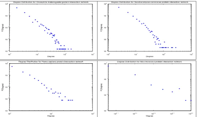
Figure 3.2 Example of degree distributions used for Euclidean distance, Kullback–Leibler divergence, Chi-square test, Pearson correlation, and Spearman Rank correlation for topology-based scoring between pairs ofk-hop subgraphs. The x-axis is the degree of a node and the y-axis is the number of nodes with that degree (P(Degree)). As can be seen from the figure, the pro-tein interaction networks exhibit scale-free like behavior as described by Barabasi and Oltvai (17) . . . 34
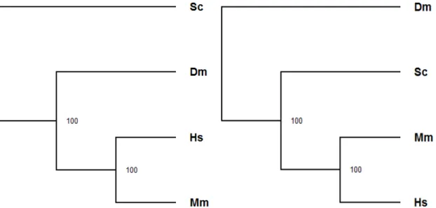
Figure 3.3 Comparison of bootstrapped trees constructed based on the labeled alignment using the KL scoring function(left)and the purely topolog-ical global comparison using the same scoring function(right)between human (Hs), mouse (Mm), yeast (Sc) and fly (Dm) . . . 43
Figure 4.1 A schematic of the graph representation of the BLAST orthologs based on protein-protein interaction networks and gene coexpression networks. The networks are represented as two labeled graphs (G1 and G2) with corresponding relationships among their nodes (similarly colored nodes are sequence homologous according to a BLAST search). Nodes from G1 (e.g., v3) are compared to their sequence-homologous counterparts in G2 (e.g., v’2 and v’6) based on the topology of their neighborhood and sequence homology of the neighbors. In the figure, v’2 has the same number of neighbors of v3 and one of the neighbors of v’2 (i.e., v’3) is sequence-homologous to v4. Thus, v’2 is scored higher (more likely to be an ortholog to v3) compared to v’6. Protein-protein interaction networks are represented as unweighted graphs, while gene coexpression networks incorporate weights (as calculated by correlations) into their edges . . . 61
Figure 4.2 An example of the graph matching conducted by the shortest path graph kernel. Similarly colored nodes are sequence homologous according to a BLAST search. As can be seen from the figure, the graph kernel compares the lengths of the shortest paths around homologous vertices across the two graphs (taking into account the weights of the edges, if available). The red edges show the matching shortest path in both graphs as computed by the graph kernel. The shortest path distance graph kernel takes into account the sequence homology score for the matching vertices across the two graphs as well as the distances between the two matched vertices within the graphs . . . 62
Figure 4.3 An example of the graph matching conducted by the random walk graph kernel. Similarly colored vertices are sequence homologous according to a BLAST search. As can be seen from the figure, the graph kernel com-pares the neighborhood around the starting vertices in each graph using random walks (taking into account the weights of the edges, if available). Colored edges indicate matching random walks across the two graphs of up to length 2. The random walk graph kernel takes into account the sequence homology of the vertices visited in the random walks across the two graphs as well as the general topology of the neighborhood around the starting vertex . . . 63
Figure 4.4 A sample 1 hop neighborhood around one of the matched orthologs (TNF receptor-associated factor 2 “P39429” in mouse and “Q12933” in human) according to the graph features (left: 1 hop network around the “P39429” protein for mouse, right: 1 hop neighborhood around the “Q12933” protein for human). Similarly colored nodes are sequence homologous. The graph properties search for similar topology and se-quence homology around the neighborhood of the nodes being compared 64
Figure 5.1 Clustering Based on Toplogical Features (Degree Distribution). Ligand networks with a high number of differentially expressed genes relative to untreated samples (as indicated in (104)) have been highlighted in the figure. . . 84
Figure 5.2 Bootstrapped tree showing the relationship between all 33 ligand net-works. This tree shows that ligands with similar induced reaction (e.g., LPS and SDF, both affect pathways involved in cell migration) cluster together. . . 85
Figure 5.3 Consensus tree constructed based on all metabolism pathways in Ta-ble 2. The values on the branches indicate the total number of times the branch appeared across all networks (total of 19). If no value is indicated, the branch appeared only once. . . 86
Figure 5.4 Consensus tree constructed based on all Genetic Information Processing pathways in Table 2. The values on the branches indicate the total number of times the branch appeared across all networks (total of 15). If no value is indicated, the branch appeared only once. . . 87
Figure 5.5 Consensus of all pathway categories in Table 2. The values on the branches indicate the total number of times the branch appeared across all networks (total of 7). If no value is indicated, the branch appeared only once. . . 88
Figure 5.6 A: Consensus tree constructed based on all Cellular Processes pathways in Table 2. B: Consensus tree constructed based on all Environmental Information Processing pathways in Table 2. C: Consensus tree con-structed based on all Human Diseases pathways in Table 2. D: Con-sensus tree constructed based on all Immune System pathways in Table 2. The values on the branches indicate the total number of times the branch appeared across all networks (totals of 10, 2, 12, and 4 forA,B, C, and D respectively). If no value is indicated, the branch appeared only once. . . 89
Figure 6.1 Left: Sample format for specifying the topology of a weighted, undi-rected network in CSV format. This file format can be generated by Cytoscape (similar to Simple Interaction File (SIF) format). The sepa-rators can be commas or any whitespace (e.g., space or tab) character. Right: Visualization of the network described by the file on the left . 97
Figure 6.2 Main alignment parameters on the input screen of the BiNA webserver 97
Figure 6.3 Overview diagram of BiNA’s service-oriented architecture model . . . . 99
Figure 6.4 BiNA’s scalability on multiple processors as measured by speedup. As can be seen from the figure, the implementation of the algorithm is highly scalable, allowing full utilization of additional processors with little performance penalty . . . 100
Figure A.1 Example of Degree distributions used for Kolmogorov-Smirnov test for initial clustering of the ligands based on network topology. As can be seen from the figure, the expression networks exhibit scale-free like behavior as described by Barabsi and Oltavai (17). . . 107
Figure A.2 Consensus tree constructed based on all KEGG pathways in TableA.1
in supplementary material. The values on the branches indicate the total number of times the branch appeared across all networks (total of 11). If no value is indicated, the branch appeared only once. . . 108
Figure A.3 Consensus tree constructed based on all Organismal System pathways in table 2 in the supplementary material (table 2 in the paper). The values on the branches indicate the total number of times the branch appeared across all networks (total of 6). If no value is indicated, the branch appeared only once. . . 109
ACKNOWLEDGEMENTS
As the saying goes: Nanos Gigantium Humeris Insidentes1. This work would not have been possible if I had not stood upon the shoulders of gentle giants. Without my advisor, Dr. Vasant Honavar, this dissertation would not have taken shape. His insight, patience and focus have been unparalleled and have inspired me to contribute all that I have to the pursuit of knowledge. My co-major advisor, Dr. Heather Greenlee, has been instrumental in the development and discussion of all the algorithms and techniques in this dissertation. Her contributions have been instrumental to chapters 2 and 4 of this dissertation. I am also thankful to Dr. Drena Dobbs, on whose shoulders I stood upon to further my understanding of protein structures and their interactions, documented in three publications early in my research career. I am in debt to Dr. Robert Jernigan, who inspired chapter 3 of this dissertation and guided me in exploring the relationship between mathematics and data in my research. I am also thankful to continuous discussions and insights with Dr. Christopher Tuggle. Such collaborations gave fruition to ideas described in chapter 4 of this dissertations.
I would also like to take this opportunity to thank the two giants in my life, my dad Dr. George Towfic and my mom Dr. Samira Kettoola, who raised me and my siblings to always pursue knowledge in all its forms. The support of my brother, Zaid, and my sister, Farah, have been instrumental during turbulent times.
Of course, I cannot begin to measure the value of the numerous discussions I’ve had with friends and colleagues regarding research, life and the interactions of those concepts: Cornelia Caragea, Oliver Couture, Yasser El-Manzalawy, Bob Farnham, Ataur Katebi, Neeraj Kaul, Sumudu Leelananda, Harris Lin, Sender Lkhagvadorj, Olga Nikolova, Dr. Don Sakaguchi, Dr. Jeanne Serb, Adrian Silvescu, Jivko Sinapov, Jia Tao, Dr. Jeff Trimarchi, John Van Hemert, Rasna Walia, Li Xue, Oksana Yakhnenko, Xia Zhang and Michael Zimmermann.
1
ABSTRACT
Comparative analyses of biomolecular networks constructed using measurements from different con-ditions, tissues, and organisms offer a powerful approach to understanding the structure, function, dynamics, and evolution of complex biological systems. The rapidly advancing field of systems biology aims to understand the structure, function, dynamics, and evolution of complex biological systems in terms of the underlying networks of interactions among the large number of molecular participants in-volved including genes, proteins, and metabolites. In particular, the comparative analysis of network models representing biomolecular interactions in different species or tissues offers a powerful means of identifying conserved modules, predicting functions of specific genes or proteins and studying the evolution of biological processes, among other applications.
The primary focus of this dissertation is on the biomolecular network alignment problem: Given two or more networks, the problem is to optimally match the nodes and links in one network with the nodes and links of the other. We describe a suite of modular, extensible, and efficient algorithms for aligning biomolecular network models including: (1) undirected graphs in their weighted and unweighted variations (2) undirected graphs in their labeled and unlabeled variants. The resulting algorithms have been implemented as part of the Biomolecular Network Alignment (BiNA) Toolkit, an open source, user-friendly suite of software for comparative analysis of networks.
Our experiments show that BiNA is (i) competitive with the state-of-the-art network alignment tools with respect to the quality of alignments (based on a variety of performance measures) and (ii) able to align large networks ranging in size from a few hundreds of nodes and a few thousand edges to tens of thousands of nodes with millions of edges. We describe several applications of BiNA including (1) construction of phylogenetic trees based on protein-protein interaction networks, and (2) identification of biochemical pathways involved in ligand recognition in B cells by aligning gene co-expression networks constructed from mRNA profiles of B cells exposed to different ligands.
CHAPTER 1. INTRODUCTION
1.1 Overview of network models and systems biology
Biological processes are orchestrated by networks of interactions among nucleic acids, pro-teins, metabolites and other ligands, both within and between cells, in response to internal or external stimuli. Recently, several high-throughput techniques have emerged for measuring gene expression under different conditions or perturbations, interactions among proteins, and among genes, proteins, regulatory RNAs, small ligands and other signaling agents. Thus, it has become possible to make system-wide measurements of biological variables (45; 84; 126). Against this background, network models of protein-protein interactions (144; 78; 156), regula-tory relationships between genes (38), metabolic pathways (80), and their combinations (5; 12) have been successfully applied in the rapidly expanding field of systems biology (29; 165). Nu-merous studies have successfully utilized network models to: comprehend how temporal and spatial clusters of genes, proteins, and signaling agents correspond to genetic, developmental and regulatory networks (160; 85; 137); uncover the biophysical basis and essential macro-molecular sequence and structural features of such interactions (147; 109); infer interactions between proteins in a target species based on experimentally characterized interactions in a source species (169); discover conserved pathways among different species (88; 145); find pro-tein groups that are relevant to disease (77; 108); predict propro-tein function (172; 92); discover the chemical mechanism of metabolic reactions (134; 91); discover topological and other char-acteristics of biomolecular networks (94; 86; 87); and explain the emergence of systems-level properties of networks from the interactions among their parts (1; 16; 17). Furthermore, driven by the need for computational tools for exploiting network models in biological sciences, sev-eral groups have developed databases for storing networks (12; 109; 8) and query languages
and tools for retrieving networks that match specified criteria (140; 109); identifying optimal matches for a source pattern e.g., a set of proteins linked by an undirected path (89; 140) or those that form a specific pattern or motif (14; 15) in one or more target networks; and for align-ing protein-protein interaction networks (89; 97; 81; 56; 149), regulatory networks (169; 139) and metabolic networks (127; 6).
Because the available data is often of variable quantity, quality and granularity, there is a need for several classes of network models at varying levels of abstraction, to explore different questions in diverse applications. Of particular interest are:
• Undirected graphsin which nodes represent genes or proteins and links between nodes denote interactions (e.g., protein-protein interaction networks (144; 78; 156)). Such net-works provide a global picture of gene-gene or protein-protein interactions that can further be analyzed to identify putative functional modules (144; 78; 156), nodes that play im-portant roles (e.g., hubs) (79); or to determine topological features (degree distribution, hierarchical structure, modularity, etc. (51; 132; 168; 90)). Comparative analysis of two or more networks of the same type from different species can help identify conserved functional modules (139; 145; 114; 170; 121), transferring functional annotations across species, etc. Although most of the work has focused on undirected graphs with a single type of links, many applications call for network models that can accommodatemultiple types of links (e.g., interaction, co-localization, etc. in the case of protein-protein interac-tion networks), ormultiple types of nodes(e.g., in the case of networks that simultaneously model the interactions among proteins, RNA, DNA, etc.), orboth.
• Undirected weighted graphse.g., gene coexpression networks in which the nodes rep-resent genes and weights on the links model the similarity of expression patterns between genes (e.g., gene expression correlation networks (145)). Such networks can be analyzed to identify clusters of genes that display similar expression patterns, e.g., using spectral clustering techniques (158; 98; 119); Comparative analysis of two or more networks from different tissues from the same species can be used to identify key differences in gene co-expression patterns; Comparative analysis of gene coco-expression networks obtained under
comparable conditions from different species can be used as a basis of inferring functional similarities between the corresponding genes, etc.
• Directed graphsthat model influences between genes where nodes represent genes and directed, unlabeled or labeled links denote regulatory interactions. Pathway databases such as TRANSPATH (99), PathCase (48), and KEGG (84) present examples of richly an-notated directed graphs. Tracing of directed paths in such graphs can uncover sequences of regulatory events, redundant regulatory mechanisms, etc; directed cycles indicate feed-back regulation. Comparison of pathways can reveal common subgraphs, putative evo-lutionary relations, etc. Topological analysis can reveal the distributions and average numbers of regulators per gene.
• Undirected or directed multi-graphs where the each node and each edge has as-sociated with it a set of labels (e.g., nodes labeled with their Gene ontology functional annotation, subcellular localization, etc.) as well as their weightedcounterparts.
The primary focus of this dissertation is on modular algorithms that are equally applicable to aligning undirected graphs and undirected, weighted graphs. The algorithms may also be extended to deal with directed graphs or multigraphs (see chapter 7 for more details).
1.2 The network alignment problem
Network alignment methods present a powerful approach for detecting conserved modules across several networks constructed from different species, conditions or timepoints. The detec-tion of conserved network modules may allow the discovery of disease pathways, proteins/genes critical to basic biological functions, and the prediction of protein functions. The problem of aligning two networks, in the absence of the knowledge of how each node in one network maps to one or more nodes in the other network, requires solving the subgraph isomorphism problem, which is known to be computationally intractable (NP-complete) (61). Consequently, several heuristics have been explored for striking a balance between the speed, accuracy and robust-ness of the alignment of large biological networks. For instance, The PathBLAST algorithm
searches for nodes/proteins that share sequence homology and the same order in the two path-ways being aligned. The runtime complexity of this algorithm, which is factorial in the length of the pathways being aligned, prevents it from being viable for aligning large networks with thousands of nodes (140). MaWISh (97) is a pairwise network alignment algorithm with a runtime complexity ofO(mn) (wherem and nare the number of vertices in the two networks being compared) that relies on a scoring function that takes into account protein duplication events as well as interaction loss/gain events between pairs of proteins to detect conserved protein clusters.
Bruckner et al.’s algorithm (Torque) attempts to address the problem whereby the topology among the nodes for the query network is not known (28). The running time complexity of Torque isO(3km) wherekis the number of vertices in the query andmis the number of edges. Hopemap is an iterative clustering-based alignment algorithm for protein-protein interaction networks. HopeMap starts by clustering homologs based on their sequence similarity and al-ready known KEGG Orthology status. The algorithm then proceeds to search for strongly connected components and outputs the conserved components that satisfy a predefined user threshold (149). Graemlin 2.0 is a linear time algorithm that relies on a feature-based scor-ing function to perform an approximate global alignment of multiple networks. The scorscor-ing function for Graemlin 2.0 takes into account protein deletion, duplication, mutation, presence and count as well as edge/paralog deletion across the different networks being aligned (56). NetworkBLAST-M (81) is a progressive multiple network alignment algorithm that constructs a layered alignment graph, where each layer corresponds to a network and edges between lay-ers connect homologs across different networks. Highly conserved subnetworks from networks from different species are first aligned based on highly conserved orthologous clusters, then the clusters are expanded using an iterative greedy local search algorithm (81).
In the following sections, we provide a detailed sketch of the network alignment algorithms that have been proposed in the literature. We also provide an analysis of the running time complexity for each of the algorithms. Finally, we provide a statement for the significance of efficient network alignment algorithms and how such algorithms may be used to address important biological questions.
1.3 Formal mathematical definition of network alignment
The graphs dealt with in this section are node-labeled, undirected and unweighted. A graph G(V, E, ρ) consists of a sets of vertices V and edges E and vertex label function ρ. V denotes {v1, v2, v3, ...vn}and E denotes{e1, e2, e3, ...ek}, wherek≤ n(n
−1)
2 . ρ is a function that assigns
labels to the vertices of G. We match labels of nodes/vertices across protein-protein interaction networks from different species using BLAST (3). H(V2, E2, ρ2) is said to be a subgraph of G(V1, E1, ρ1) if V2 ⊂V1,ρ2(i) =ρ1(i) ∀i ∈V2, and E2 ⊂E1 where E2 consists only of edges
whose end points are in V2. We associate with the graphs G1(V1, E1, ρ1) and G2(V2, E2, ρ2)
sets subgraphs S1 = {C1, C2, C3, ...Cn} and S2 = {Z1, Z2, Z3, .., Zm}(respectively), where
Ci(Ki, Oi, µi) 1 ≤ i ≤ n is a subgraph of G1 and Zj(Wj, Qj, κj) 1 ≤ j ≤ m is a subgraph of G2. Our basic strategy is to find a best match for each subgraph in S1 from S2 by
op-timizing a scoring function, K(Ci, Zi), such that we obtain: (i) a set of vertices that satisfy
µi(u) =κj(v), where v ∈Wj and u ∈Ki (ii) a set of edges whereby: if (µi(u1), µi(u2)) is an
edge inOi, then (κj(v1), κj(v2)) is an edge inQj whereµi(u1) =κj(v1) andµi(u2) =κj(v2). In
this section, we present two different choices of graph kernels forK(Ci, Zj): the shortest path kernel (22) and random walk kernel (157). The resulting solution to the network alignment problem satisfies the condition that each subgraph inS1 has at most one matching subgraph in S2. Thus, a pairwise alignment of the networks G1(V1, E1, ρ1) and G2(V2, E2, ρ2) is expressed
in terms of an optimal alignment among the sets of the corresponding sets of subgraphs in S1
and S2.
1.4 Brief overview of state-of-the-art methods 1.4.1 MaWISh
MaWISh (Maximum-Weight Induced Subgraph) is a local pairwise alignment algorithm for protein-protein interaction networks that focuses on discovering highly conserved subgraphs in the interactome of a pair of species. The problem is modeled as a graph optimization problem, while taking into account duplication/divergence models (see Figure 1.1). It is a greedy algorithm that finds a set of nodes in each graph such that the alignment score is
Figure 1.1 Original figure from Koyuturk et al. (97). The Duplica-tion/Elimination/Emergence model considered in MaWISh. Starting with three interactions between three proteins, protein u1 is duplicated to add u1 into
the network together with its interactions (dashed circle and lines). Then, u1 loses
its interaction with u3 (dotted line). Finally, an interaction between u1 and u1 is
added to the network (dashed line)
highest. Specifically, MaWISh searches for hubs in a graph, then adds neighbors to each hub based on a heuristic that measures the conservation of the module across several graphs. The runtime complexity of MaWISh is O(mn) (where m and n are the number of vertices in the two networks being compared).
1.4.2 NetworkBLAST-M
Kalaev et al.’s extension to the NetworkBLAST algorithm to align multiple protein-protein interaction networks consists of stacking the protein-protein interaction networks in to multiple layers, then connecting the nodes across the layers (using inter-layer edges) using sequence homology based on a pre-computed phylogenetic tree. The algorithm searches for high scoring subnets (multiple k-spines, see Figure 1.2) and outputs the high scoring subnets as possible alignments across the various input networks from different species. The algorithm starts by computing a seed subnetwork that consists of 2 spines, then expands the alignment iteratively around the seed spines. The initial seed spines are found by imposing a strict topology on the connected nodes from each species. For example, in Figure 1.2, although there is no edge connecting the nodes in species U1 and U2, the nodes are still reachable from each other due to
the fact that there is a path from U1 to U3 and from U3 to U2. The seed searching algorithm
assumes that such a topology is equivalent to the case where there are edges connecting the nodes from U1to U2and from U2to U3. Furthermore, the algorithm assumes that a homologous
protein must exist in every species/network in the alignment. Thus the k-spines contain k
proteins, one from every species in the alignment. The seed spines are expanded by searching for spines that contain only nodes that are at most two hops away from the seed spines.
1.4.3 Graemlin
Graemlin is a linear time Multiple Alignment algorithm for protein-protein interaction net-works that relies on a parameter-learning algorithm to decompose netnet-works into specific feature vectors and compute the similarity based on such features. Graemlin also provides a parameter-learning algorithm that can automatically weight the contribution of each feature based on a precomputed alignment. The features for nodes considered in Graemlin 2.0 are:
• Protein presence (the maintenance of proteins in both species)
• Protein count (the maintenance of more than one protein in both species) • Protein deletion (the loss of a protein in one of the two species)
• Protein duplication (the duplication of a protein in one of the two species) • Protein mutation (the divergence in sequence of two proteins in different species) • Paralog mutation (the divergence in sequence of two proteins in the same species) The features considered for edges in Graemlin 2.0 are:
• Edge deletion (the loss of an interaction between two pairs of proteins in different species) • Paralog edge deletion (the loss of an interaction between two pairs of proteins in the same
species)
Graemlin 2.0 relies on a phylogenetic tree to sum the pairwise features over pairs of species adjacent in the tree, including ancestral species. The feature functions also take into account the evolutionary distance between the species being compared (see Figure 1.3).
1.4.4 GRAAL
GRAph ALigner (GRAAL) is a strictly topological alignment algorithm that relies on graphlet distributions to compare networks (101). GRAAL has been successfully utilized for reconstructing phylogenetic relationships between bacterial species based on the topologies of the species’ protein-protein interaction networks. Briefly, GRAAL relies on the computation of graphlets up to four nodes in size around each node between the graphs being compared. Each node in a network is given a score denoting how many graphlets they participate in. The scores for nodes across two networks are then compared using Milenkoviæ et al.’s (115) formula for averaging node-based scores in a graph:
S(u1x, vy2) = |log(S(u
1
x) + 1)−log(S(vy2) + 1)| log(max(S(u1
x), S(v2y)) + 2)
Where S(u1x) and S(vy1) are the scores for the nodes from G1(V1, E1) and G2(V2, E2), where u1x ∈ V1 and v2y ∈ V2. The above formula produces a normalized score for each node-based
graphlet score.
1.5 Limitations of current methods
Current approaches to biomolecular network alignment summarized above suffer from sev-eral limitations: Most of the biomolecular network alignment algorithms described above deal with a specific type of network (e.g., protein-protein interaction networks). Because the scoring functions for matching nodes across networks, or for aligning the networks based on matches between nodes across networks, and the heuristics used to speed up the alignment are typically hard-coded into the implementation of the respective algorithms, it is not straightforward to extend the existing implementations (e.g., for aligning protein-protein interaction networks) to handle more general classes of biomolecular networks (e.g., networks that model multiple types of interactions between multiple types of molecular entities). Nor is it easy to replace or modify specific components of the alignment algorithms (e.g., the scoring function used for matching nodes across networks) to meet the needs of specific biological applications, or to easily specify at runtime the specific characteristics of the biomolecular networks that can be exploited by
the alignment algorithm (73; 142). Some of the algorithms, because of computational consid-erations, make some simplifying assumptions that are at odds with the known characteristics of biomolecular networks (142).
1.6 Significant contributions of dissertation
This dissertation provides a class of flexible (in terms of ease of modification), scalable (in terms of computational running time), and accurate (in terms of biological significance) algo-rithms for comparing and aligning biomolecular networks while making minimum assumptions about the source of the networks. The networks can be labeled (e.g., sequence labeled, or nodes can be matched based on orthology) or unlabeled (networks can be aligned strictly based on topology). The following sections describe the main contributions of this dissertation against the background of the current literature in the field.
1.6.1 First highly modular algorithm in the field
Chapter 2 describes the Biomolecular Network Alignment (BiNA) toolkit in detail. This algorithm is the first algorithm in the field whose scoring (comparison) functions and partition (clustering) functions are independent. Furthermore, this algorithm uses the proven divide and conquer strategy to enable the future addition of new techniques for partitioning and scoring without changing the overall method.
1.6.2 Highly scalable algorithm
BiNA can run on desktop machine to clusters, aligning networks from 100’s of edges to several millions. Chapter 6 describes the implementation details and scalability of the algorithm in detail. The running time of the various methods that comprise this algorithm are described in detail in chapter 2.
1.6.3 First highly flexible algorithm
BiNA can align undirected, unweighted protein interaction networks and undirected, weighted gene-coexpression networks. BiNA can align within the same organism or across species, can
align based on topology alone or using node labels or BLAST correspondence. Experiments on aligning networks from different species are provided in chapters 2, 3 and 4. Experiments outlining the alignment of networks within the same organism are provided in chapter 5. The alignment techniques based on strict topology and discussion of applications of topology to the alignment problem are provided in chapter 3.
1.6.4 Highly portable
BiNA has been implemented purely in Java to achieve maximum portability on Windows, Mac and Linux/Unix systems). The BiNA webserver is user-friendly and accessible. The architecture and implementation of the algorithm are discussed in chapter 6.
1.6.5 High accuracy in terms of biological performance
BiNA has been evaluated in several respects to assess the biological relevance of the algo-rithm’s output. Several assessments currently available in the literature are:
• Detection of enriched GO Terms (chapters 2 and 3)
• Construction of phylogenies based on labeled and unlabeled protein-protein interaction networks (chapter 3)
• Detection of orthologs (chapter 4)
1.6.6 Applied to important biological problems
BiNA has been applied to several important biological questions. Two of the applications currently available in the literature are:
• Detection of orthologs based on protein-protein and gene coexpression networks (chapter 4)
Figure 1.2 Slightly modified figure from Kalaev et al. (81). A seed defined by a
d-identical-spine subnet (d = 3 in the above example since there are 3 k-spines), where thek-spines are restricted to be paths with identical topology. The dashed blue line encloses one of the three k-spines. The phylogenetic tree used to order the connection operation of the inter-layer edges of the k-spines is shown at the top of the figure
Figure 1.3 Original figure from Flannick et al. (56). This figure shows the set of evolutionary events that are computed by Graemlin’s node and edge feature functions. Graemlin 2.0 uses a phylogenetic tree with branch lengths to determine the events. First, the species weight vectors (shown as gray boxes) at each internal node of the tree are constructed; the weight vector represents the similarity of each extant species to the internal node. Graemlin 2.0 uses these weight vectors to compute the likely evolutionary events (shown as black boxes) that occur
CHAPTER 2. BIOMOLECULAR NETWORK ALIGNMENT (BiNA) TOOLKIT
Based on a paper titled ”Aligning Biomolecular Networks using Modular Graph Kernels”, accepted for publication in WABI 20091
Fadi Towfic, M. Heather West Greenlee and Vasant Honavar
Abstract
Comparative analysis of biomolecular networks constructed using measurements from differ-ent conditions, tissues, and organisms offer a powerful approach to understanding the structure, function, dynamics, and evolution of complex biological systems. We explore a class of algo-rithms for aligning large biomolecular networks by breaking down such networks into subgraphs and computing the alignment of the networks based on the alignment of their subgraphs. The resulting subnetworks are compared using graph kernels as scoring functions. We provide im-plementations of the resulting algorithms as part of BiNA, an open source biomolecular network alignment toolkit. Our experiments usingDrosophila melanogaster,Saccharomyces cerevisiae,
Mus musculus andHomo sapiens protein-protein interaction networks extracted from the DIP repository of protein-protein interaction data demonstrate that the performance of the pro-posed algorithms (as measured by % GO term enrichment of subnetworks identified by the alignment) is competitive with some of the state-of-the-art algorithms for pair-wise alignment of large protein-protein interaction networks. Our results also show that the inter-species sim-ilarity scores computed based on graph kernels can be used to cluster the species into a species tree that is consistent with the known phylogenetic relationships among the species.
2.1 Background and Motivation
The rapidly advancing field of systems biology aims to understand the structure, func-tion, dynamics, and evolution of complex biological systems (29). Such an understanding may be gained in terms of the underlying networks of interactions among the large number of molecular participants involved including genes, proteins, and metabolites (165; 62). Of particular interest in this context is the problem of comparing and aligning multiple networks e.g., those generated from measurements taken under different conditions, different tissues, or different organisms (139). Network alignment methods present a powerful approach for detect-ing conserved modules across several networks constructed from different species, conditions or timepoints. The detection of conserved network modules may allow the discovery of disease pathways, proteins/genes critical to basic biological functions, and the prediction of protein functions.
The problem of aligning two networks, in the absence of the knowledge of how each node in one network maps to one or more nodes in the other network, requires solving the subgraph isomorphism problem, which is known to be computationally intractable (NP-Hard) (61). How-ever, in practice, it is possible to establish correspondence between nodes in the two networks to be aligned and to design heuristics that strike a balance between the speed, accuracy and ro-bustness of the alignment of large biological networks. For instance, MaWISh (97) is a pairwise network alignment algorithm with a runtime complexity ofO(mn) (wheremandnare the num-ber of vertices in the two networks being compared) that relies on a scoring function that takes into account protein duplication events as well as interaction loss/gain events between pairs of proteins to detect conserved protein clusters. Hopemap (149) is an iterative clustering-based alignment algorithm for Protein-Protein Interaction networks. HopeMap starts by clustering homologs based on their sequence similarity and already known KEGG/InParanoid Orthology status. The algorithm then proceeds to search for strongly connected components and outputs the conserved components that satisfy a predefined user threshold (149). Graemlin 2.0 is a lin-ear time algorithm that relies on a feature-based scoring function to perform an approximate global alignment of multiple networks. The scoring function for Graemlin 2.0 takes into account
protein deletion, duplication, mutation, presence and count as well as edge/paralog deletion across the different networks being aligned (56). NetworkBLAST-M (81) is a progressive mul-tiple network alignment algorithm that constructs a layered alignment graph, where each layer corresponds to a network and edges between layers connect homologs across different networks. Highly conserved subnetworks from networks from different species are first aligned based on highly conserved orthologous clusters, then the clusters are expanded using an iterative greedy local search algorithm (81).
Against this background, we explore a class of algorithms for aligning large biomolecular networks using adivide and conquer strategy that takes advantage of themodularsubstructure of biological networks (67; 132; 70). The basic idea behind our approach is to align a pair of networks based on the optimal alignments of the subnetworks of one network with the subnet-works of the other. Different ways of decomposing a network into subnetsubnet-works in combination with different choices of measures of similarity between a pair of subnetworks yield different algorithms for aligning biomolecular networks.
We utilize variants of state-of-the-art graph kernels (22; 23), first developed for use in training support vector machines for classification of graph-structured patterns, to compute thesimilarity between two subgraphs. The use of graph kernels to align networks offers several advantages: It is easy to substitute one graph kernel for another (to incorporate different application-specific criteria) without changing the overall approach to aligning networks; it is possible to combine multiple graph kernels to create more complex kernels (23) as needed. Our experiments with the fly, yeast, mouse and human protein-protein interaction networks extracted from DIP (Database of Interacting Proteins) (136) demonstrate the feasibility of the proposed approach for aligning large biomolecular networks.
The rest of the paper is organized as follows: Section 2 precisely formulates the problem of aligning two biomolecular networks and describes the key elements of our proposed solution. Section 3 describes the experimental setup and experimental results. Section 4 concludes with a summary of the main contributions of the paper in the broader context of related literature and a brief outline of some directions for further research.
2.2 Problem Formulation
We consider the problem of pair-wise alignment of protein-protein interaction networks. We model protein interaction networks as undirected and unweighted graphs. In a protein-protein interaction network, the vertices in the graph correspond to protein-proteins and the edges denote interactions between the two proteins. Let the graphsG1(V1, E1) andG2(V2, E2) denote
two protein-protein interaction networks whereV1={v11, v12, v31, ...vn1}andV2 ={v12, v22, v32, ...v2m}, respectively, denote the vertices ofG1 and G2; and E1 and E2 denote the edges of G1 and G2
respectively. Let a matrixP with|V1|rows and |V2|columns (i.e,n×m matrix) denote a set
of matches between the vertices of G1 and G2. The mapping matrix P is defined such that
for any two vertices vx1 and v2y (where 1 ≤ x ≤ n and 1 ≤ y ≤ m) from graphs G1 and G2,
respectively, Pv1
xvy2 = 1 if v
1
x from G1 is matched to vy2 from G2 and Pv1
xv2y = 0 if v
1
x in G1 is
not a match tovy2 inG2. For example, the matches between nodes may be based on homology
between the sequences of the corresponding proteins. Thus, each node in G1 is matched to 0
or more nodes ofG2 and vice versa. Note that the number of such matches for any node inG1
is much smaller than the total number of nodes inG2 and vice versa.
C1(L1, O1) is said to be a subgraph of G1(V1, E1) if L1 ⊂ V1 and O1 ⊂ E1 where O1
consists only of edges whose end points are in L1. We associate with the graphs G1(V1, E1)
and G2(V2, E2) sets of subgraphs S1 ={C1, C2, C3, ...Cl} and S2={Z1, Z2, Z3, .., Zw} (respec-tively), whereCi(Li, Oi) 1≤i≤lis a subgraph ofG1 andZj(Wj, Qj) 1≤j≤wis a subgraph ofG2. Our basic strategy is to find a best match for each subgraph inS1fromS2 by optimizing
a scoring function,K(Ci, Zj), such that we obtain: (i) a set of vertices that satisfyPv1
xvy2 = 1,
where vx1 ∈ Li and vy2 ∈ Wj and (ii) a set of edges where: if (v1x, v1d) is an edge in Oi, then (vy2, vg2) is an edge inQj wherePv1
xv2y = 1 andPv1dv2g = 1. The resulting solution to the network
alignment problem satisfies the condition that each subgraph in S1 has at most one matching
subgraph in S2. Thus, a pairwise alignment of the networks G1(V1, E1) and G2(V2, E2) is
ex-pressed in terms of an optimal alignment among the sets of the corresponding sets of subgraphs inS1 andS2.
2.3 Algorithm 2.3.1 Divide: Partitioning methods
As noted earlier, our basic approach to aligning a pair of protein-protein interaction net-works involves (a) decomposing each network into a collection of smaller subnetnet-works; (b) compute the alignment of the two networks in terms of the optimal alignments of the sub-networks of one network with the subsub-networks of the other. Different choices of methods for decomposing a network into subnetworks in combination with different choices of measures of
similarity between a pair of subnetworks yield different algorithms for aligning protein-protein interaction networks. In our current implementation, we establish the matches between nodes in the two protein-protein interaction networks to be aligned based on reciprocal BLASTp (3) hits between the corresponding protein sequences. Thus, Pv1
xvy2 = 1 if and only if the
corre-sponding protein sequences of vx1 and vy2 are reciprocal BLASTp hits (74) for each other (at some chosen user-specified threshold). Alternatively, the mapping can be established based on known homologies (e.g between the human WNT1 and mouse Wnt1 proteins) (96; 30).
2.3.1.1 K-Hop
Ak-hop neighborhood-based approach to alignment uses the notion ofk-hop neighborhood. The k-hop neighborhood of a vertex v1x ∈V1 of the graphG1(V1, E1) is simply a subgraph of G1that connectsvx1 with the vertices inV1 that are reachable ink hops fromvx1 using the edges inE1. Given two graphs G1(V1, E1) andG2(V2, E2),a mapping matrix Pthat associates each
vertex inV1 with zero or more vertices inV2 and a user-specified parameterk, we construct for
each vertexvx1∈V1 its correspondingk-hop neighborhoodCx inG1. We then use the mapping
matrix P to obtain the set of matches for vertex vx1 among the vertices in V2; and construct
the k-hop neighborhood Zy for each matching vertex v2y in G2 and Pv1
xvy2 = 1. Let S(v
1
x, G2)
be the resulting collection of k-hop neighborhoods in G2 associated with the vertexvx1 inG1.
We compare eachk-hop subgraph Cx inG1 with each member of the corresponding collection S(vx1, G2) to identify thek-hop subgraph ofG2that is the best match forCx (based on a chosen similarity measure). This process is illustrated in figure 2.1. The runtime complexity of the
Figure 2.1 General schematic of the k-hop neighborhood alignment algorithm. The input to the algorithm are two graphs (G1 and G2) with corresponding relationships
among their nodes using mapping matrix P(similarly colored nodes are sequence homologous according to a BLAST search, for examplePv2v0
6 = 1). The algorithm
starts at an arbitrary vertex inG1(red vertex in the figure) and constructs ak-hop
neighborhood around the starting vertex (1-hop neighborhood in the figure). The algorithm then matches each of the nodes in the 1-hop neighborhood subgraph from G1 to nodes inG2 using mapping matrixP. 1-hop subgraphs are then constructed
around each of the matching vertices. The 1-hop subgraphs from G2 are then
compared using a scoring function (e.g. a graph kernel) to the 1-hop subgraph from G1 and the maximum scoring match is returned.
k-hop neighborhood based network alignment algorithm is O(bmg) where m is the number of nodes in the query network G1, b is the maximum number of matches in the target network G2 for any node in the query network, andg is the running time of the similarity measure or
scoring function used to compare a pair of k-hop subnetworks.
2.3.1.2 Decomposing Networks Into Clusters
A graph clustering based alignment algorithm works as follows: Given two node-labeled graphs G1(V1, E1) and G2(V2, E2),and a mapping matrix P that associates each vertex inV1
with zero or more vertices inV2, we first extract collections of subgraphsH1 ={C1, C2, C3, ...Cl} and H2 ={Z1, Z2, Z3, ...Zw} from G1 and G2 respectively. In principle, any graph clustering
Figure 2.2 Schematic for the cluster-based alignment algorithm. The input to the algorithm are two graphs (G1 and G2) with corresponding relationships among their nodes
using mapping matrixP(similarly colored nodes are sequence homologous accord-ing to a BLAST search, for example Pv2v20 = 1). Subgraphs are generated from
G1 and G2 using a graph clustering algorithm (e.g. bicomponent clusterer that
finds biconnected subgraphs) and the subgraphs from G1 are compared against
the subgraphs from G2 to find the best matching subgraphs using an appropriate
scoring function.
algorithm may be used to construct the subgraph sets H1 and H2. In our experiments, we
used the bicomponent clusterer as implemented in the JUNG (Java Universal Network/Graph) framework (123; 163) to extractH1 and H2. Briefly, the bicomponent clusterer searches for all
biconnected components (graphs that cannot be disconnected by removing a single node/vertex (68)) by traversing a graph in a depth-first manner (please see (111) for more details). Once the subgraph sets H1 and H2 of the biconnected subgraphs of G1 and G2 (respectively) are
extracted, an all vs. all comparison is conducted to identify for each subgraph inH1, the best
matching subgraph in H2 using a scoring function (e.g. a graph kernel, see figure 2.2). The
running time complexity of this algorithm isO(lwg) wherelis the number of clusters extracted from the query networkG1,wis the number of clusters extracted from the target network G2 ,
2.3.2 Conquer: Scoring Functions
We now proceed to describe the similarity measures or scoring functions used to compare a pair of subgraphs (e.g., a pair ofk-hop subgraphs or a pair of bi-component clusters described above).
2.3.2.1 Shortest Path Graph Kernel
The shortest path graph kernel was first described by Borgwardt and Kriegel (22). As the name implies, the kernel compares the length of the shortest paths between any two nodes in a graph based on a pre-computed shortest-path distance. The shortest path distances for each graph may be computed using the Floyd-Warshall algorithm as implemented in the CDK (Chemistry Development Kit) package (143). We modified the Shortest-Path Graph Kernel to take into account the sequence homology of nodes being compared as computed by BLAST (3). The shortest path graph kernel for subgraphsZG1 andZG2 (e.g.,k-hop subgraphs, bicomponent
clusters extracted fromG1 and G2 respectively) is given by:
K(ZG1, ZG2) = log X v1 i,v1j∈ZG1 X v2 k,v2p∈ZG2 δ(vi1, v2k)×δ(vj1, vp2)×d(v1i, v1j)×d(v2k, vp2) (2.1) where δ(vx1, v2y) = BlastScore(v 1 x,v2y)+BlastScore(v2y,vx1) 2 . d(v 1
i, vj1) and d(v2k, vp2) are the lengths of the shortest paths between vi1,vj1 and v2k,v2p computed by the Floyd-Warshall algorithm. The runtime of the Floyd-Warshall Algorithm is O(n3). The shortest path graph kernel has a runtime of O(n4) (wherenis the maximum number of nodes in larger of the two graphs being compared). Please see figure2.3for a general outline of the comparison technique used by the shortest-path graph kernel.
2.3.2.2 Random Walk Graph Kernel
The random walk graph kernel (157) has been previously utilized by Borgwardt et al. (23) to compare protein-protein interaction networks. The random walk graph kernel for subgraphs ZG1 and ZG2 (e.g., k-hop subgraphs, bicomponent clusters extracted from G1 and G2
respec-Figure 2.3 An example of the graph matching conducted by the shortest path graph kernel. Similarly colored nodes are sequence homologous according to a BLAST search. As can be seen from the figure, the graph kernel compares the lengths of the shortest paths around homologous vertices across the two graphs. The red edges show the matching shortest path in both graphs as computed by the graph kernel. The shortest path distance graph kernel takes into account the sequence homology score for the matching vertices across the two graphs as well as the distances between the two matched vertices within the graphs.
tively) is given by:
K(ZG1, ZG2) =p×(I−λKx)
−1×q (2.2)
whereIis the identity matrix,λis a user-specified variable controlling the length of the random walks (a value of 0.01 was used for the experiments in this paper), Kx is an nm×nm matrix (where n is the number of vertices in ZG1 and m is the number of vertices in ZG2 resulting
from the Kronecker productKx=ZG1⊗ZG2, specifically,
Kαβ =δ(ZG1ij, ZG2kl), α≡m(i−1) +k, β≡m(j−1) +l (2.3)
Whereδ(ZG1ij, ZG2kl) =
BlastScore(ZG1ij,ZG2kl)+BlastScore(ZG2kl,ZG1ij)
2 ;p and q are 1×nmand nm×1 vectors used to obtain the sum of all the entries of the inverse expression ((I−λKx)−1). We adapted the random walk graph kernel to align protein-protein interaction networks by taking advantage of the reciprocal BLAST hits (RBH) among the proteins in the networks from different species (74). Naive implementation of our modified random-walk graph kernel, like the original random-walk graph kernel (157), has a runtime complexity of O(r6) (where r=max(n, m)). This is due to the fact that the product graph’s adjacency matrix isnm×nm,
Figure 2.4 An example of the graph matching conducted by the random walk graph kernel. Similarly colored vertices are sequence homologous according to a BLAST search. As can be seen from the figure, the graph kernel compares the neighborhood around the starting vertices in each graph using random walks. Colored edges indicate matching random walks across the two graphs of up to length 2. The random walk graph kernel takes into account the sequence homology of the vertices visited in the random walks across the two graphs as well as the general topology of the neighborhood around the starting vertex.
and the matrix inverse operation takesO(h3) time, wherehis the number of rows in the matrix being inverted (thus, the total runtime isO((rm)3) or O(r6) wherer =max(n, m)). However, runtime complexity of the random walk graph kernel (and hence our modified random walk graph kernel) can be improved toO(r3) by making use of the Sylvester equations as proposed by Borgwardt et al. (23). Figure 2.4 illustrates the computation of the random walk graph kernel.
2.3.2.3 Page Rank (topology based)
Based on the work of Brin and Page (27) and implemented in the Java Universal Net-work/Graph Framework (123), the Page Rank score is calculated by first constructing a func-tion measuring the transifunc-tion probability around each nodeu in the undirected graphG(V, E) as (1−α)∗ 1 degree(u) +α∗ 1 |V|
where|V|is the number of nodes/vertices inG,degree(u) is the number of neighbors of nodeu and α is a constant parameter describing the influence from each nodeu. In our experiments,
α is set to 0.15. For nodes with no neighrbors, degree1 (u) is set to 0. The transition probability of the Markov chain is then used to calculate the stationary probability of transitioning to each node in the graph. Thus, this scoring function compares the transition probabilities around each node in the graphs being compared and outputs a high score for graphs that have similar topologies as measured by their transition probabilities and a low score otherwise.
2.3.2.4 Kullback–Leibler divergence of degree distributions (topology based) In lieu of the Euclidean distance function used above, the Kullback–Leibler (KL) divergence (103) can be used to calculate the difference between the two degree distributions from thek -hop subgraphs H(Q, W) and K(R, T). First, the degree distributions from the graphs are converted to n-dimentional vectors h and k, respectively and the KL divergence between the distributions can then be calculated as follows:
n X i=1 hi sum(h)log2 hi sum(h) ki sum(k) !
The advantage of this approach is that it is not as sensitive as Euclidean distance to bin size or size of the graph due to the normalization procedure required to convert the degree frequencies to probabilities. It is also relatively quick to calculate compared to the Random Walk and Shortest Path Distance graph kernels.
2.3.2.5 Chi-square test between degree distributions (topology based)
The chi-square test (141) can also function as a similarity measure between degree distribu-tions. The degree distributions from thek-hop subgraphsH(Q, W) andK(R, T) are converted ton-dimentional vectorsh andk, respectively and Pearson’s cumulative test statistic is calcu-lated between the distributions as follows:
n
X
i=1
ki−hi
hi
Although this approach is slightly sensitive to large differences in the sizes of the graphs being compared, it provides a rigid statistical comparison between the distributions and is less
likely to be skewed by slight fluctuations between the degree distributions.
2.3.2.6 Pearson correlation between degree distributions (topology based) Pearson’s product moment correlation coefficient measures the linear dependence between the two degree distributions represented as n-dimentional vectors h and k from the k-hop subgraphs H(Q, W) andK(R, T). Pn i=1(hi−h¯)(ki−k¯) q Pn i=1(hi−h¯)2 q Pn i=1(ki−k¯)2
2.3.2.7 Spearman Rank correlation between degree distributions (topology based)
Spearman’s rank correlation measures the linear dependence between the ranks of the n -dimentional vectors h and k from the k-hop subgraphs H(Q, W) and K(R, T). This non-parametric correlation measure is more robust in dealing with frequency distributions that may have a large discrepancy in their frequencies compared to their ranks. Spearman’s rank correlation is defined as
1− 6 Pn
i=1d2i
n(n2−1)
Wheredi is defined as the difference between the ranks of the raw frequency countshi and
ki
2.4 Summary and Discussion
Aligning biomolecular networks from different species, tissues and conditions allows of-fers a powerful approach to discover shared components that can help explain the observed phenotypes. Specifically, applications of network alignment allow the discovery of conserved pathways among different species (88; 145), finding protein groups that are relevant to dis-ease (77; 108), discovery of the chemical mechanism of metabolic reactions (134; 91) and more
(172; 92; 137; 17; 1). We have explored a novel class of graph kernel based polynomial time al-gorithms for aligning biomolecular networks. The proposed alal-gorithms align large biomolecular networks by decomposing them into easy to compare substructures. The resulting subnetworks are compared using graph kernels as scoring functions. The modularity of kernels (35) offers the possibility of constructing composite kernel functions using existing kernel functions that capture different but complementary notions of similarity between graphs (23).
The runtime complexity of the k-hop neighborhood based alignment algorithm isO(bmg) where m is the number of nodes in the query network G1, b is the maximum number of
matches in the target networkG2 for any node in the query network, andgis the running time
of the similarity measure or scoring function used to compare a pair ofk-hop subnetworks. The running time complexity of this algorithm isO(lwg) wherelis the number of clusters extracted from the query networkG1,wis the number of clusters extracted from the target networkG2,
andgis the running time of the scoring function used to compare a pair of clusters (subgraphs). In comparison, the run-time complexity of NetworkBLAST-M (O((np)ds3s)), where n is the number of nodes in each of the networks, sthe number of networks, pan upper bound on the node degree anddthe number ofseed spinesused to generate the alignment. In the special case of pairwise network alignment (s=2), the run-time complexity of NetworkBLAST reduces to O((np)d).The runtime complexity of HopeMap is linear in terms of the total number of nodes and edges in the alignment graph (149), which is O(2n+ 2n2) in terms of the input graphs (where each input graph has at most n nodes).
The k-hop network neighborhood based and bicomponent clustering based protein-protein interaction network alignment algorithms are implemented in BiNA (http://www.cs.iastate. edu/~ftowfic), an open source Biomolecular Network Alignment toolkit. The current imple-mentation includes variants of the shortest path and random walk graph kernels for computing similarity between pairs of subnetworks. The modular design of BiNA allows the incorporation of alternative strategies for decomposing networks into subnetworks and alternative similarity measures (e.g., kernel functions) for computing the similarity between subnetworks. Some in-teresting directions for further work on the biomolecular network alignment algorithms include: • Design of alternative measures of performance for assessing the quality of the generated
network alignments.
• Algorithms for aligning networks that contain directed links, such as transcriptional reg-ulatory networks, multiple types of nodes (proteins, DNA, RNA) and multiple types of links.
• Extensions that allow the alignment of multiple networks.
• The use of more sophisticated graph-clustering algorithms (such as MCL (49)).
• Automated tuning of parameters (e.g λ for the random walk kernel) using parameter learning techniques (56).
• Optimizations that reduce the runtime memory requirements of the algorithm.
Acknowledgments
This research was supported in part by an Integrative Graduate Education and Research Training (IGERT) fellowship to Fadi Towfic, funded by the National Science Foundation grant (DGE 0504304) to Iowa State University and a National Science Foundation Research Grant (IIS 0711356) to Vasant Honavar. The authors are grateful to the WABI-09 anonymous referees for their helpful comments on the manuscript.


![Análise automática de aspectos relacionados a coerência semântica em resumos acadêmicos (Automatic Analysis of Semantic Coherence Aspects in Academic Abstracts) [in Portuguese]](data:image/gif;base64,R0lGODlhAQABAIAAAP///wAAACH5BAEAAAAALAAAAAABAAEAAAICRAEAOw==)