Efficient online evaluation of big data stream classifiers

Efficient Online Evaluation of Big Data Stream Classifiers

Albert Bifet

Noah’s Ark Lab HUAWEI Hong Kong [email protected]

Gianmarco

De Francisci Morales

Jesse Read

Geoff Holmes,

Bernhard Pfahringer

ABSTRACT

The evaluation of classifiers in data streams is fundamen-tal so that poorly-performing models can be identified, and either improved or replaced by better-performing models. This is an increasingly relevant and important task as stream data is generated from more sources, in real-time, in large quantities, and is now considered the largest source ofbig data. Both researchers and practitioners need to be able to effectively evaluate the performance of the methods they em-ploy. However, there are major challenges for evaluation in a stream. Instances arriving in a data stream are usually time-dependent, and the underlying concept that they represent may evolve over time. Furthermore, the massive quantity of data also tends to exacerbate issues such as class imbalance. Current frameworks for evaluating streaming and online al-gorithms are able to give predictions in real-time, but as they use a prequential setting, they build only one model, and are thus not able to compute the statistical significance of results in real-time. In this paper we propose a new evalu-ation methodology for big data streams. This methodology addresses unbalanced data streams, data where change oc-curs on different time scales, and the question of how to split the data between training and testing, over multiple models.

Categories and Subject Descriptors

H.2.8 [Database Management]: Database Applications -Data Mining

Keywords

Data Streams, Evaluation, Online Learning, Classification

Permission to make digital or hard copies of all or part of this work for personal or classroom use is granted without fee provided that copies are not made or distributed for profit or commercial advantage and that copies bear this notice and the full citation on the first page. Copyrights for components of this work owned by others than the author(s) must be honored. Abstracting with credit is permitted. To copy otherwise, or republish, to post on servers or to redistribute to lists, requires prior specific permission and/or a fee. Request permissions from [email protected].

Copyright is held by the owner/author(s). Publication rights licensed to ACM. ACM 978-1-4503-3664-2/15/08$15.00.

DOI: http://dx.doi.org/10.1145/2783258.2783372.

1.

INTRODUCTION

Data is flowing into every area of our life, both professional and personal. There is no consensus on the definition of big data, however a popular definition describes it as data whose characteristics put it beyond the ability of typical tools to capture, manage, and analyze, due to time and memory con-straints [21]. This need has spurred a considerable amount of research in data mining and machine learning, aimed at extracting information and knowledge from big data.

In this paper, we focus on the evaluation of classifiers in a big data setting such as the one provided by Apache SAMOA1[9] i.e., classifying evolving data streams in a

dis-tributed fashion. When the classification algorithm runs on top of a distributed system, we can leverage its process-ing power to train multiple classifiers and provide statistical significance to the evaluation procedure. There is no pre-vious work that describes an evaluation methodology that gives statistically significant results in streaming classifica-tion, going beyond the standard prequential setting which builds only one model for the evaluation. Providing sta-tistical significance is of paramount importance in order to ensure that evaluation results are valid and not misleading. Evaluation is a delicate task that has generated numerous controversies [14, 18]. As mentioned by Japkowicz and Shah [18], having a standard evaluation approach can be linked to the desire of having an “acceptable” scientific practice in the field. Unfortunately, researchers often achieve such acceptability by taking shortcuts. The problem with this practice is that the comparisons of algorithms’ performance, although appearing acceptable, are frequently invalid. In this paper we highlight the importance of a proper evalua-tion methodology for streaming classifiers, and contribute to this discussion by presenting some insightful results. From these, we develop and present some effective new proposals. To motivate the need for this discussion, we present three striking cases of misleading evaluation (details in§4 and§5): • by comparing two classifiers applied to data streams, we show that one of them is statistically significantly bet-ter than the other by using McNemar’s test. However, the two classifiers are actually two instances of the same algorithm, randomized ensembles of decision trees, each seeded with a different number. A test such as

McNe-1

http://samoa-project.net KDD '15, August 10-13, 2015, Sydney, NSW, Australia.

mar’s, which works properly for small datasets, is mis-leading when used with larger ones. Nevertheless, this test is commonly used for data stream classification [24]; • splitting data into several disjoint datasets for training seems reasonable for large datasets [11]. Unfortunately, this type of partitioning leads to an evaluation procedure that cannot distinguish between classifiers that ought to perform differently by design;

• a simple majority class classifier that keeps the majority class of a sliding window may have positive κ statistic and positive harmonic mean accuracy for some periods. Learning from evolving data streams is quite different from learning from traditional batch data. Standard cross-validation techniques do not apply, due to the fact that data instances can be strongly time-dependent, and classifiers also evolve along with the data. It is no use training a classi-fier on a large number of data instances, and then evaluating it on some following data (analogous to a static train/test split) without letting classifiers evolve with the new data. In a big data stream scenario, the instances in the test set could be millions of instances away from the ones used to train the model. A classifier may be built using some features as the most relevant, but when the data changes, the classifier has to adapt and choose new relevant features. It is therefore useful to have a statistically valid way to measure the per-formance of classifiers at any time. Current frameworks for data streams such as MOA2 [3], VFML3 [16], and Vowpal Wabbit4_{[20] provide only single fold prequential evaluation.}

Therefore, they fall short of a statistically sound evaluation setting.

In this work we identify a set of currently popular ap-proaches that are problematic, highlight the issues arising from the big data streaming setting, and finally propose some solutions. Specifically, we tackle the following issues: I1. Validation methodology. Prequential evaluation, the

most commonly used evaluation in stream learning, uses examples first to test and then to train a single model. This method is unable to provide statistical significance when comparing classifiers. On the other hand, the most common error estimation technique for the batch setting, cross-validation, is not directly ap-plicable in streaming.

I2. Statistical testing. McNemar’s test, which has been proposed as one of the best tests for streaming, is mis-leading.

I3. Unbalanced measure. Common measures of perfor-mance such as F1 and Accuracy are biased toward one class.

I4. Forgetting mechanism. The most popular approaches, sliding window and exponential forgetting, are both parametric with difficult to choose parameters. In ad-dition, they allow a mix of distributions in the input window.

To address these issues we propose: a new prequential bootstrap validation to address I1; to use the Sign test or

2

http://moa.cms.waikato.ac.nz

3_{http://www.cs.washington.edu/dm/vfml} 4

http://hunch.net/~vw

the Wilcoxon signed-rank test to address I2; a new measure for accuracy performance,κmstatistic to address I3, and a

new forgetting mechanism for prequential evaluation based onADWINto address I4.

This paper is structured as follows. We present some re-lated work in Section 2, distributed validation methodologies in Section 3, statistical tests in Section 4, evaluation perfor-mance measures in Section 5, and a real-time prequential measure in Section 6. Finally, Section 7 presents some con-cluding remarks.

2.

RELATED WORK

The most important reference in evaluating data streams is by Gama et al. [13]. The paper mainly discusses static streams, and how to extend the static streaming prequential evaluation to evolving data streams using a sliding window or a fading factor.

Dietterich [11] reviewed five approximate statistical tests for determining whether one learning method out-performs another on a particular classification task. These tests were compared experimentally to check the type I and type II errors on the differences. The main conclusion was that 5x2 cross validation test was recommended, due to it being slightly more powerful than McNemar’s test.

Bouckaert [6] recommends using the 10x10 cross valida-tion test where all individual accuracies are used to estimate the mean and variance and with 10 degrees of freedom for binary data. It has the same properties as other calibrated repeated k-fold cross validation tests, and he showed that it empirically outperforms 5x2 cross validation, (corrected) resampling and k-fold cross validation on power and repli-cability.

Demsar [10] reviewed statistical tests for comparing more than two algorithms on multiple datasets. One of his propos-als is to use the Friedman test with a corresponding post-hoc test, that we discuss in more detail in Section 4.

Shah [25] proposed a new agreement statistic that is a generalization of the Cohen’s kappa statistic to the case of multiclass classification by a fixed group of experts. The proposed generalization reduces to the classical version of Cohen’s kappa statistic in the case of binary classification by two experts. Its main advantage is that it yields tighter agreement assessments, due to its accounting for expert spe-cific biases and correlations.

More generally, the recent book by Japkowicz and Shah [18] is a complete and updated reference for classification evaluation.

3.

METHODS FOR VALIDATION

The validation procedure for a learning algorithm deter-mines which examples are used for training, and which are used for testing the learned model.

In traditional batch learning the problem of limited avail-ability of data is overcome by analyzing and averaging mul-tiple models produced with different random arrangements of training and test data. In the stream setting the problem of (effectively) unlimited data poses different challenges.

In the literature there are two main approaches to evaluate data streams:

• prequential evaluation, averaging ten experiments when learners or streams are randomly generated, and when it is possible to vary their random seeds; otherwise by

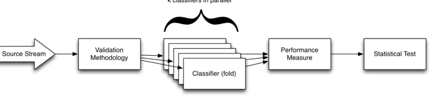
Source Stream Validation Methodology

Classifier (fold)

Performance

Measure Statistical Test

}

k classifiers in parallel

Figure 1: Block diagram of the proposed evaluation pipeline for big data stream classifiers.

using only one experiment with real data datasets and non randomized classifiers;

• standard 10-fold cross-validation, to compare with other batch methods.

The former cannot be used to obtain statistical signif-icance of results when using real datasets with any non-randomized classifier. Furthermore, this strategy is not amenable to parallelization. The latter treats each fold of the stream independently, and therefore may miss concept drift occur-ing in the data stream.

To overcome these problems, we discuss the following strate-gies. Assume we havek different instances of the classifier we want to evaluate running in parallel. The classifier does not need to be randomized. Each time a new example ar-rives, it is used in one of the following ways:

• k-fold distributed cross-validation: each example is used for testing in one classifier selected randomly, and used for training by all the others;

• k-fold distributed split-validation: each example is used for training in one classifier selected randomly, and for testing in the other classifiers;

• k-fold distributed bootstrap validation: each ex-ample is used for training in each classifier according to a weight from a Poisson(1) distribution. This results in each example being used for training in approximately two thirds of the classifiers, with a separate weight in each classifier, and for testing in the rest.

The first approach is an adaptation of cross-validation to the distributed streaming setting. It makes maximum use of the available data at the cost of high redundancy of work.

The split-validation approach has the advantage of cre-ating totally independent classifiers, as they are trained on disjoint parts of the stream. However, this approach poten-tially underutilizes available data.

The last approach simulates drawing random samples with replacement from the original stream. This approach is also used in online bagging [23, 22].

All three strategies have a corresponding prequential ver-sion, where training examples are first used for testing.

A high level block diagram of the whole evaluation pipeline is shown in Figure 1.

3.1

Streaming Setting

In the streaming setting, classifiers and streams can evolve over time. As a result, the performance measures of these classifiers can also evolve over time. Given this dynamic

na-ture, it is interesting to be able to evaluate the performance of several classifiers online.

For simplicity, let us assume a binary classification prob-lem. The ideal setting for evaluation when data is abundant is the following: let X be the instance space, let Dt be a

distribution over X and time, let ft be a target function

ft :X → [0,1], and letct be a model evolving over time,

so that it can be different at each time instant t. A clas-sifier C is a learning algorithm that produces a hypothesis ct:X→[0,1].

We are interested in obtaining its errorec(t)(x) =|ct(x)−

ft(x)|, which also depends on time. The true error is ¯ec(t)=

Ex∈D[ec(t)(x)]. Let the error discrepancy be the difference

between the true and estimated error. Ink-fold evaluation the estimated error is the average over all fold estimates.

3.2

Theoretical Insights

Let us mention here two important theoretical results.

Theorem 1. (Test Set Lower Bound)[19] For all classi-fiersc,mtest instances, and for allδ∈(0,1], the following holds:

Pr(|true error - est. error| ≤

r ln(2/δ)

2m )≥1−δ In other words, with the same high probability, having more instances will reduce the discrepancy between the true error and the estimated error, which, in our case, suggests that a prequential strategy (using the instances for testing before training) improves the estimation of the true error.

Following the approach by Blum et al. [5], the second re-sult is that the discrepancy between true error and estimated error is reduced using ak−fold strategy.

Theorem 2. ∀q ≥ 1, E[|true error - est. error|q

] is no larger for the prequentialk−fold strategy than for a prequen-tial evaluation strategy, i.e.,

E[|true errork−estimated errork|q]≤

E[|true error1−estimated error1|q]

In other words, usingk−fold prequential evaluation is bet-ter than using only prequential evaluation, and gives us the-oretical ground for addressing issue I1. Given the inter-dependence between validation methodology and statistical tests, we defer experimental evaluation to Section 4.

Table 1: Comparison of two classifiers with Sign test and Wilcoxon’s signed-rank test.

Class. A Class. B Diff Rank

77.98 77.91 0.07 4 72.26 72.27 -0.01 1 76.95 76.97 -0.02 2 77.94 76.57 1.37 7 72.23 71.63 0.60 5 76.90 75.48 1.42 8 77.93 75.75 2.18 9 72.37 71.33 1.04 6 76.93 74.54 2.39 10 77.97 77.94 0.03 3

4.

STATISTICAL TESTS FOR COMPARING

CLASSIFIERS

The three most used statistical tests for comparing two classifiers, are the following [18]:

• McNemar. This test is non-parametric. It uses two variables: the number of examples misclassified by the first classifier and correctly classified by the second a, and the number of examples classified the opposite way b. Hence, it can be used even with a single-fold validation strategy. The McNemar statistic (M) is computed as M =sign(a−b)×(a−b)2/(a+b). The statistic follows the χ2 _{distribution under the null hypothesis that the}

two classifiers perform equally well.

• Sign test. Is also non-parametric but uses the results at each fold as a trial. As such, it cannot be used with a standard prequential strategy. It computes how many times the first classifier outperforms the second classifier, and how many times the opposite happens. The null hypothesis corresponds to the two classifiers performing equally, and holds if the number of wins follows a bino-mial distribution. If one of the classifiers performs better on at leastwαfolds, then it is considered statistically

sig-nificantly better at the αsignificance level, wherewα is

the critical value for the test at theαconfidence level. • Wilcoxon’s signed-rank test. Is also non-parametric,

and uses the results at each fold as a trial. For each trial it computes the difference in performance of the two clas-sifiers. After ranking the absolute values of these differ-ences, it computes the sum of ranks where the differences are positive, and the sum of ranks where the differences are negative. The minimum value of these two sums is then compared to a critical value Vα. If this minimum

value is lower, the null hypothesis that the performance of the two classifiers is the same can be rejected at the αconfidence level.

Consider the following example: two classifiers have 10 performance measures, one for each fold, as shown in Ta-ble 1. Classifier A outperforms classifier B in eight folds. Using the sign-test, given that forα=.05 we havewα= 8,

we can reject the null hypothesis that the two classifiers perform similarly at theα=.05 confidence level. To apply the Wilcoxon’s signed-rank test, first we rank the absolute values of the differences between the two classifiers’ perfor-mances. Then we compute the sum of ranks where the dif-ferences are positive (53), and the sum of ranks where the

differences are negative (3). We compare the minimum of these two sums (3) to a critical valueVα= 8 at theα=.05

confidence level. As 3 is lower than 8, we reject the null hypothesis that the the two classifiers perform equally well. This procedure can be extended to compare multiple clas-sifiers. Demsar [10] proposes to use the Friedman test with a corresponding post-hoc test, such as the Nemenyi test. Let rj_i be the rank of the j-th of k classifiers on the i-th of N datasets. The average rank of the j-th classifier is Rj = 1/nP_irji. The Nemenyi test is the following: two

classifiers are performing differently if the corresponding av-erage ranks differ by at least the critical difference

CD=qα

r

k(k+ 1) 6N

where k is the number of classifiers, N is the number of datasets, and critical valuesqαare based on the Studentized

range statistic divided by√2.

4.1

Type I and II Error Evaluation

AType I error or false positive is the incorrect rejection of a true null hypothesis, in our case, that two classifiers have the same accuracy. Our experimental setting is the following: we have a data stream, and we use it as input to classifiers that have the same accuracy by design since they are built using the same algorithm. Then, we check which evaluation methodology is better at avoiding the detection of a difference between statistically equally-performing clas-sifiers, i.e., which method has a lower type I error.

We run an experiment following the methodology pre-sented by Dietterich [11], and build randomized classifiers with different seeds. We use two different models trained with random forests [4], and compare them with the statis-tical tests discussed in this Section.

A Type II error or false negative is the failure to reject a false null hypothesis, in our case, to detect that two clas-sifiers have different accuracy. For detecting this type of error, we perform the following experiment. We have a data stream that we use to feed a set of classifiers. These clas-sifiers have different accuracy performance by design. We build this set of classifiers by using a base classifier and ap-plying a noise filter. The noise filter changes the class label of each example prediction of the classifier with probability pnoise. For acclass problem, if the accuracy of the original

classifier isp0, the filtered classifier has an accuracy of:

p=p0×(1−pnoise) + (1−p0)×pnoise/c

since p will be p0 minus the correctly predicted examples

that have switched their label (p0×pnoise), plus the incorrect

predicted examples that due to the switch of the class label, are now correct (1−p0)×pnoise/c. Given that

∆p pnoise = p0−p pnoise = (c+ 1)p0−1 c ,

pwill be lower thanp0 whenp0>1/(c+ 1).

Experimental Setting. We compare 10-fold distributed evaluation with the non prequential and prequential ver-sions, and with split-validation, cross-validation, and boot-strapping over 50 runs at theα= 0.05 confidence level.

We use synthetic and real datasets. Synthetic data has several advantages: it is easier to reproduce and there is little cost in terms of storage and transmission. We use the data

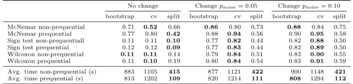
Table 2: Average fraction of null hypothesis rejection for different combinations of validation procedures and statistical tests, aggregated over all datasets. The first column group concerns Type I errors, and the other two column groups concern Type II errors.

No change Changepnoise= 0.05 Changepnoise= 0.10

bootstrap cv split bootstrap cv split bootstrap cv split McNemar non-prequential 0.71 0.52 0.66 0.86 0.80 0.73 0.88 0.84 0.75 McNemar prequential 0.77 0.80 0.42 0.88 0.94 0.56 0.90 0.95 0.58 Sign test non-prequentiall 0.11 0.11 0.10 0.77 0.82 0.44 0.82 0.88 0.50 Sign test prequential 0.12 0.12 0.09 0.77 0.83 0.44 0.82 0.89 0.50 Wilcoxon non-prequential 0.11 0.11 0.14 0.79 0.84 0.51 0.83 0.90 0.55 Wilcoxon prequential 0.11 0.10 0.19 0.80 0.84 0.54 0.83 0.91 0.59 Avg. time non-prequential (s) 883 1105 415 877 1121 422 900 1148 421 Avg. time prequential (s) 813 1202 109 820 1214 111 808 1294 112

generators with concept drift most commonly found in the literature: SEA Concepts Generator [26], Rotating Hyper-plane [17], Random RBF Generator, and LED Generator [7]. The UCI machine learning repository [1] contains some real-world benchmark data for evaluating machine learning tech-niques. We consider two of the largest: Forest Covertype, and Poker-Hand. In addition, we consider the Electricity dataset [15, 12]. Experiments can be replicated with the open-source frameworkApache SAMOA[9].

A summary of results is shown in Table 2. The values show the average fraction of repetitions that detect a dif-ference between the two classifiers, i.e., that reject the null hypothesis. Ideally, the value should be close to zero when the classifiers are the same (first column group), and close to one when the two classifiers are different (second and third column groups). Overall, the best validation procedure is cross-validation, closely followed by bootstrap, while split-validation performs the worst. For Type II errors, most statistical tests perform comparably when using a good val-idation method (cv or bootstrap), i.e., the tests detect the presence of the additional noise. Conversely, for Type I er-rors there is a large performance gap. McNemar’s test is clearly misleading as it detects a non-existent difference at least 42% of the time, while in fact the two classifiers are built by the same algorithm.

Table 3 shows a breakdown of the results for McNemar’s test on each dataset. It is evident that the test has a ten-dency to overestimate the statistical difference of two clas-sifiers. On the other hand, Table 4 shows the results for Wilcoxon’s signed-rank test for all data streams. This test is more discriminative than the Sign test, and the best strate-gies are still cross-validation and bootstrap. In most cases (with the exception of the SEA generator), Wilcoxon’s test has perfect accuracy for Type II errors, and very high accu-racy for Type I errors (≤10% average error).

A plausible explanation for the difference among the dif-ferent validation procedures is rooted in the number of ex-amples that each classification algorithm uses to build the model. In 10-fold split validation, the models are built on 10% of the examples, in 10-fold cross validation, the mod-els are built on 90% of the examples, and in bootstrap, the models use 63.2% of the examples (on average). The ex-periments show that building the models in each fold with more examples helps to determine whether the classifiers are statistically different, for both Type I and Type II errors.

In terms of efficiency, by looking at the average time of the experiments in Table 2, we conclude that bootstrapping is the most efficient methodology, as it is the one with the best ratio of discriminative power against resources consumed.

There is little difference in the results between the pre-quential and non-prepre-quential version of the experiments. The prequential version has the advantage that models do not need to receive separate examples for testing, only re-ceiving training examples is enough.

Based on these results, we recommend the prequentialk -fold distributed bootstrap validation procedure as the most efficient methodology to address issue I1. We also recom-mend avoiding McNemar’s test, and using Wilcoxon’s signed-rank test to address issue I2.

The main intuition behind the inappropriateness of Mc-Nemar’s test lies in its use of examples rather than folds as the unit of its statistical treatment. Given that in a stream the number of examples (sample size) is virtually unbounded, the statistical power of the test (its sensitiv-ity) becomes very high, and also susceptible to small dif-ferences in performance (magnitude of the effect) caused by random fluctuations. Tests using folds as their statistical unit, such as Wilcoxon’s, are thus inherently more robust, as their power is fixed by the configuration, rather than in-creasing with the number of examples in the stream. Of course, folds are not independent of each other, and the number of folds affects the minimum detectable difference. This statistical dependence is likely the reason behind the residual Type I and Type II errors in our analysis, although further study is needed to characterize its effect.

5.

UNBALANCED PERFORMANCE

MEA-SURES

In real data streams, the number of examples for each class may be evolving and changing. Theprequential error is computed based on an accumulated sum of a loss function Lbetween the predictionyt and observed values ˆyt:

p0=

n

X

t=1

L(ˆyt, yt).

However, the prequential accuracy measure is only appro-priate when all classes are approximately balanced [18].

In the following we review standard approaches to eval-uation in imbalanced data, then we point out some prob-lems with this methodology, and propose a new one, which we later demonstrate in experiments to be a more accurate gauge of true performance.

5.1

The Kappa Statistic

When the data stream is unbalanced, simple strategies that use this fact may have good accuracy. A way to take

Table 3: Fraction of null hypothesis rejection on each dataset when using McNemar’s test. Values for the best performing validation method (closest to zero for Type I errors, closest to one for Type II errors) are shown in bold.

No change Changepnoise= 0.05 Changepnoise= 0.10

bootstrap cv split bootstrap cv split bootstrap cv split

CovType 0.86 0.64 0.98 0.97 0.98 0.98 0.98 0.99 0.99 Electricity 0.45 0.16 0.79 0.99 0.92 0.88 1.00 1.00 0.94 Poker 0.73 0.45 0.86 0.82 0.78 0.98 0.96 0.99 1.00 LED(50000) 0.92 0.85 0.96 0.96 0.92 1.00 0.99 0.96 1.00 SEA(50) 0.67 0.35 0.88 0.69 0.39 0.89 0.70 0.43 0.89 SEA(50000) 0.68 0.35 0.89 0.70 0.41 0.89 0.71 0.44 0.89 HYP(10,0.001) 0.61 0.32 0.61 1.00 1.00 1.00 1.00 1.00 1.00 HYP(10,0.0001) 0.61 0.40 0.83 1.00 1.00 1.00 1.00 1.00 1.00 RBF(0,0) 0.89 0.80 0.36 0.98 0.98 0.39 0.99 0.99 0.40 RBF(50,0.001) 0.26 0.20 0.36 0.18 0.43 0.39 0.20 0.44 0.39 RBF(10,0.001) 0.88 0.74 0.36 0.97 0.96 0.39 0.98 0.98 0.40 RBF(50,0.0001) 0.76 0.68 0.37 0.91 0.76 0.39 0.91 0.76 0.41 RBF(10,0.0001) 0.89 0.80 0.36 0.96 0.92 0.37 0.98 0.94 0.40 Average 0.71 0.52 0.66 0.86 0.80 0.73 0.88 0.84 0.75

Table 4: Fraction of null hypothesis rejection on each dataset when using Wilcoxon’s Signed-Rank test. Values for the best performing validation method (closest to zero for Type I errors, closest to one for Type II errors) are shown in bold.

No change Changepnoise= 0.05 Changepnoise= 0.10

bootstrap cv split bootstrap cv split bootstrap cv split

CovType 0.12 0.10 0.10 0.99 1.00 0.63 1.00 1.00 0.97 Electricity 0.12 0.13 0.14 1.00 1.00 0.72 1.00 1.00 0.98 Poker 0.08 0.10 0.10 0.79 1.00 1.00 1.00 1.00 1.00 LED(50000) 0.11 0.09 0.10 0.82 0.49 1.00 1.00 0.99 1.00 SEA(50) 0.11 0.12 0.14 0.26 0.27 0.11 0.36 0.45 0.12 SEA(50000) 0.10 0.09 0.09 0.21 0.29 0.11 0.32 0.49 0.11 HYP(10,0.001) 0.09 0.10 0.13 1.00 1.00 1.00 1.00 1.00 1.00 HYP(10,0.0001) 0.13 0.09 0.11 1.00 1.00 1.00 1.00 1.00 1.00 RBF(0,0) 0.11 0.10 0.32 1.00 1.00 0.29 1.00 1.00 0.33 RBF(50,0.001) 0.14 0.10 0.30 0.32 1.00 0.33 0.13 1.00 0.29 RBF(10,0.001) 0.12 0.10 0.32 1.00 1.00 0.28 1.00 1.00 0.28 RBF(50,0.0001) 0.10 0.11 0.31 1.00 0.85 0.31 0.99 0.86 0.30 RBF(10,0.0001) 0.10 0.09 0.31 1.00 1.00 0.32 1.00 1.00 0.29 Average 0.11 0.10 0.19 0.80 0.84 0.54 0.83 0.91 0.59

this into account, is to normalizep0 by using

p00=

p0−minp

maxp−minp

where minp and maxp are the minimum and maximum accuracy obtainable in the stream, respectively.

TheKappa statisticκwas introduced by Cohen [8]: κ=p0−pc

1−pc

.

The quantity p0 is the classifier’s prequential accuracy,

and pc is the probability that a chance classifier–one that

assigns the same number of examples to each class as the classifier under consideration–makes a correct prediction. If the classifier is always correct thenκ= 1. If its predictions are correct as often as those of a chance classifier, thenκ= 0. For example, if a chance classifier accuracy is 0.48, and prequential accuracy is 0.65, then κ = 0.65−0.48

1−0.48 = 32.69%

(Table 5).

The efficiency of computing the Kappa statistic is an im-portant reason why it is more appropriate for data streams than a measure such as the area under the ROC curve.

Similarly, the Matthews correlation coefficient (MCC) is a correlation coefficient between the observed and predicted binary classifications defined as:

M CC= p T P·T N−F N·F P

(T P+F N)(T P+F P)(F P+T N)(F N+T N) Note that its numerator (T P·T N−F N·F P) is the de-terminant of the confusion matrix (CM D). Theκstatistic has the same numerator:

κ=p0−pc 1−pc = 2·T P·T N−F N·F P n2_(1−p c) since p0= T P+T N n pc= (T P+F N)(T P+F P) n2 + (F P+T N)(F N+T N) n2 .

This fact explains why the behavior of these two measures is so similar: they have the same zero value (T P ·T N = F N·F P), and the same two extreme values (−1 and 1).

5.2

Harmonic Mean

Unbalanced measures that use class label accuracies are thearithmetic mean and thegeometric mean

A= 1/c·(A1+A2+. . .+Ac)

G= (A1×A2×. . . Ac)1/c,

where Ai is the prequential accuracy on class i and c is

the number of classes, e.g., in a binary classification setting AC+=T P/(T P+F N). Note that the geometric accuracy

of the majority vote classifier would be zero, as accuracy on the classes other than the majority would be zero. Perfect classification yields one. If the accuracies of a classifier are balanced across the classes, then the geometric accuracy is equal to standard accuracy.

Theharmonic meanis defined as: H =c 1 A1 + 1 A2 +. . . 1 Ac . (1)

The main advantage of the harmonic mean is that, as it is always smaller than the arithmetic mean and the geometric mean (H ≤G≤A), it tends strongly toward the accuracy of the class with higher error, thus helping to mitigate the impact of large classes and emphasizing the importance of smaller ones.

Note that for a two class problem, A, G, H follow a ge-ometric progression with a common ratio of G/A ≤ 1, as G=A·(G/A),H=G·(G/A), andH=A·(G/A)2_.

This measure is inspired by theF1 measure, the harmonic mean between precision and recall:

F1 = 2

1/prec. + 1/recall =

2·T P

2T P+F N+F P, (2) where precision = _{T P}T P_{+F P} and recall = _{T P}T P_{+F N}.

Note that the F1 measure is not symmetric, as it ignores TN. We can rewriteF1, to includeT N, as

F10= 1

1 + 1/2(F N_{T P} +F P_{T N}),

which is, in fact, equivalent to the harmonic mean:

H = 2 1/_{T P}T P_{+F N}+ 1/_{T N}T N_{+F P} = _{T P+F N} 2 T P + T N+F P T N = 1 1 + 1/2(F N T P + F P T N) . As computing determinants for dimensions larger than 2 is much more expensive than computing the harmonic mean, the determinant of the confusion matrix (CM D) may be used only for binary classification, and the harmonic mean for multi-class classification.

5.3

Problems with Kappa Statistic and

Har-monic Mean

Consider the simple confusion matrix shown in Table 5. Class+is predicted correctly 40 out of 100 times, and Class-is predicted correctly 25 times. So the accuracyp0 is 65%.

A random classifier that predicts solely by chance–in the same proportions as the classifier of Table 5–will predict Class+andClass-correctly in 31.50% and 16.50% of cases

respectively. Hence, it has an accuracy pc of 48%. The κ

statistic is then 32.69%, MCC is 37.28%, the accuracy for Class+ is 57.14% and for Class-is 83.33%, the arithmetic meanAis 70.24%, the geometric meanGis 69.01% and the harmonic meanH is 67.80%.

It may seem that as theκstatistic is positive (32.69%) and harmonic mean is high (67.80%), we have a good classifier. However, if we look at the accuracy of a majority class clas-sifier that predicts alwaysClass+, it is 70.0%, sinceClass+ appears in 70% andClass-appears in 30% of examples.

It is commonly, and wrongly, assumed that theκstatistic is a measure that compares the accuracy of a classifier with the one of a majority class classifier, and that any major-ity class classifier will always haveκstatistic equal to zero. However, as we see in Table 5, this is not always the case. A majority class classifier can perform better than a given classifier while the classifier has a positiveκ statistic. The reason is that the distribution of predicted classes (45%-55%) may substantially differ from the distribution of the actual classes (70%-30%).

Therefore, we propose to use a new measure that indicates when we are doing better than a majority class classifier, and name itκmstatistic. Theκmstatistic is defined as:

κm=

p0−pm

1−pm

.

The quantity p0 is the classifier’s prequential accuracy,

andpmis the prequential accuracy of a majority class

clas-sifier. If the classifier is always correct then κm= 1. If its

predictions are correct as often as those of a majority class classifier, thenκm= 0.

In the example of Table 5, the majority classifier acquires accuracy of 0.7, and prequential accuracy is 0.65, thenκm=

0.65−0.7

1−0.7 =−16.67%. This negative value ofκm shows that

the classifier is performing worse than the majority class classifier.

In summary, we propose to use theκmstatistic to address

issue I3, a measure that is easily comprehensible, with a be-havior similar toCM Dandκ, and that deals correctly with the problems introduced by skew in evolving data streams.

5.4

Statistic Evaluation

The main motivation of using the κm statistic is when

data streams are evolving class unbalanced. We show that this measure has advantages over accuracy and κ-statistic: it is a comprehensible measure, and it has a zero value for a majority class classifier.

We perform a prequential evaluation with a sliding win-dow of 1000 examples, on theElectricity dataset, where the class label identifies the change of the price relative to a moving average of electricity demand over the previous 24 hours; with a total of 45,312 examples. This dataset is a widely used dataset described by Harries [15] and analysed

Table 5: Simple confusion matrix example. Predicted Predicted

Class+ Class- Total

Correct Class+ 40 30 70

Correct Class- 5 25 30

0 1 2 3 4 ·104 0 50 100 Time, examples H o effd in g T ree % p0 accuracy κstatistic

H harmonic accuracy κmstatistic

0 1 2 3 4 ·104 0 20 40 60 80 100 Time, examples M a jo rit y Cla ss % p0 accuracy κstatistic

H harmonic accuracy κmstatistic

Figure 2: Accuracy,κStatistic, Harmonic Accuracy, andκmStatistic of a Hoeffding Tree (left) and a Majority Class classifier

(right) on the Electricity Market Dataset.

by Gama [12]. This dataset was collected from the Aus-tralian New South Wales Electricity Market. In this market, prices are not fixed but are affected by demand and supply of the market, and are set every five minutes.

Comparing the usage ofp0,κstatistic, harmonic accuracy

Handκmstatistic (Figure 2), we see that for the Hoeffding

tree, theκmstatistic is similar or lower to theκstatistic, and

for a period of time it is negative. Negative values indicate that the Hoeffding tree is doing worse than a simple majority class classifier. This behaviour is not discovered by the other measures, thus showing the benefit of using this new κm

statistic measure.

In the right part of Figure 2, we compare the different measures for the majority class classifier that uses a sliding window of 1000 examples. Of course theκm statistic has

a constant value of zero, but the κstatistic and harmonic accuracyH have some positive values. This behavior is due to the evolution of the class labels, as at a certain point the majority switches from one label to the other. In this window theκ statistic can be positive. Again, we see the benefit of using this newκm statistic measure.

5.4.1

The Kappa-Temporal Statistic Measure

κper = p−pper 1−pper

, (3)

wherepper is the accuracy of the Persistent classifier. The Persistent classifier is a classifier that predicts that the next class label will be the same as the last seen class label.

We would like to note that κper corresponds to the κm

measure computed using a sliding window of size 1. Com-puting the majority class of a sliding window of size 1 is the same as using the last seen class label.

6.

REAL-TIME PREQUENTIAL MEASURE

The performance of a classifier may be evolving over time. We propose to evaluate learning systems using real-time measures of performance: the average of the prequential

measures in the most recent sliding window containing data that corresponds to the current distribution of data.

Holdout evaluation gives a more accurate estimation of the accuracy of the classifier on more recent data. However, it requires recent test data that it is difficult to obtain for real datasets. Gama et al. [13] propose to use a forgetting mechanism for estimating holdout accuracy by using pre-quential accuracy: a sliding window of sizewwith the most recent observations p0(t) = 1 w t X k=t−w+1 L(ˆyk, yk),

or fading factors that weigh observations using a decay fac-tor α. The output of the two mechanisms is very similar (every window of sizew0 may be approximated by some

de-cay factor α0). The authors note in their paper that ”we

observed that the choice of fading factors and the window size is critical.”

As the output will depend on the scale of change of the data stream, we propose to use accuracy and κm statistic

measured using an adaptive sliding window such as ADWIN [2], an algorithm for estimating mean and variance, detect-ing change and dynamically adjustdetect-ing the length of a data window to keep only recent data.

ADWIN keeps a variable-length window of recently seen items, for example loss function valuesL(ˆyk, yk) in a

classi-fication task, such that the window has the maximal length statistically consistent with the hypothesis “there has been no change in the average value inside the window.”

More precisely, an older fragment of the window is dropped if and only if there is enough evidence that its average value differs from that of the rest of the window. This has two consequences: one, that change is reliably declared when-ever the window shrinks; and two, that at any time the average over the existing window can be reliably taken as an estimation of the current average in the stream.

ADWINis parameter- and assumption-free in the sense that it automatically detects and adapts to the current rate of change. Its only parameter is a confidence boundδ, indicat-ing the desired confidence in the algorithm’s output, inher-ent to all algorithms dealing with random processes.

In our case, ADWIN keeps a sliding window W with the most recentxt =L(ˆyt, yt). Letn denote the length ofW,

W0·W1 a partition of W, ˆµW the (observed) average of

the elements inW, and µW the (unknown) average of µt

fort∈W.

Since the values ofµtcan oscillate wildly, there is no

guar-antee thatµW or ˆµW will be anywhere close to the

instan-taneous value µt, even for long W. However, µW is the

expected value of ˆµW, so µW and ˆµW do get close asW

grows.

Now we state our main technical result about computing prequential accuracy usingADWINbased in [2]:

Theorem 3. Letn0 andn1 be the lengths ofW0 andW1

and n be the length of W, so that n = n0+n1. Let µˆW0

andµˆW1 be the averages of the values in W0 andW1, and

µW0 andµW1 their expected values. During the evaluation,

at every time step we have:

1. (False positive rate bound). If µt remains constant

within W, the probability thatADWIN detects a change and shrinks the window at this step is at mostδ. 2. (False negative rate bound). Suppose that for some

partition ofW in two partsW0W1(whereW1 contains

the most recent items) we have |µW0−µW1|>2cut,

where

m = 1

1/n0+ 1/n1

(harmonic mean of n0 andn1),

δ0 = δ n, and cut= r 1 2m·ln 4 δ0 .

Then with probability1−δADWINdetects a change and shrinks W toW1, or shorter.

ADWIN is efficient, since the total processing time per ex-ample isO(logW) (amortized) andO(logW) (worst-case).

6.1

Prequential Evaluation

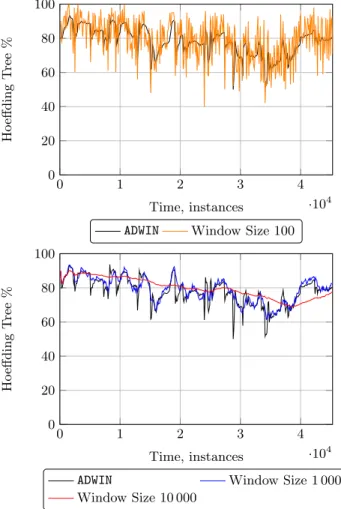
In the next experiment, we plot the prequential evaluation for three different sizes of a sliding window: 100, 1 000, and 10 000. The plots are shown in Figure 3. We observe that the plots are different depending on the size of the window. In this example, where we plot the accuracy of a Hoeffding Tree using the Electricity dataset, we see that with a size of 10 000, the plot is smoothed, with a size of 100, there are many fluctuations, and that the size that is more similar to theADWINprequential accuracy is the sliding window of size 1 000. We note that usingADWINthe evaluator does not need to choose a size for the sliding window, and that it has theoretical guarantees that the chosen size is optimal.

Figure 4 shows a comparison between a hold-out evalu-ation, a prequential evaluation usingADWIN, a sliding win-dow of 100 and a sliding winwin-dow of 10 000. We observe that the prequential evaluation using ADWINis very similar to hold-out evaluation, and that short sliding windows have some fluctuations, and large sized sliding windows may have some delay. For evolving data streams with different rates of change, the size of the optimal window is not always the same. ADWINprequential evaluation is an easy way to have an estimation similar to hold-out evaluation without need-ing testneed-ing data, and without needneed-ing to decide the optimal size of a sliding window for evaluation.

0 1 2 3 4 ·104 0 20 40 60 80 100 Time, instances H o effd in g T ree %

ADWIN Window Size 100

0 1 2 3 4 ·104 0 20 40 60 80 100 Time, instances H o effd in g T ree %

ADWIN Window Size 1 000

Window Size 10 000

Figure 3: Accuracy using a sliding window of 100, 1 000, 10 000 andADWINfor the Electricity Market Dataset

7.

CONCLUSIONS

Evaluating data streams online and in a distributed envi-ronment opens new challenges. In this paper we discussed three of the most common issues, namely: (I1) which valida-tion procedure to use, (I2) the choice of the right statistical test, (I3) how to deal with unbalanced classes, and (I4) and the proper forgetting mechanism. We gave insights into each of these issues, and proposed several solutions: prequential k-fold distributed bootstrap (I1), Wilcoxon’s signed-rank test (I2),κmstatistic (I3), andADWINprequential evaluation

(I4). This new evaluation methodology will be available in

Apache SAMOA, a new open-source platform for mining

big data streams [9].

Our main goal was to contribute to the discussion of how distributed streaming classification should be evaluated. As future work, we will extend this methodology to regression, multi-label, and multi-target learning.

0 0.2 0.4 0.6 0.8 1 ·106 20 40 60 80 Time, instances H o effd in g T ree % Hold-out ADWIN Window 100 Window 10 000 Figure 4: Prequential evaluation with several measures on a stream of a million of instances.

8.

REFERENCES

[1] A. Asuncion and D.J. Newman. UCI machine learning repository, 2007. URL

http://www.ics.uci.edu/~mlearn/MLRepository.html.

[2] Albert Bifet and Ricard Gavald`a. Learning from time-changing data with adaptive windowing. InSDM, 2007.

[3] Albert Bifet, Geoff Holmes, Richard Kirkby, and Bernhard Pfahringer. MOA: Massive Online Analysis. Journal of Machine Learning Research (JMLR), 2010. URL

http://moa.cms.waikato.ac.nz/.

[4] Albert Bifet, Geoff Holmes, and Bernhard Pfahringer. Leveraging bagging for evolving data streams. InECML PKDD, pages 135–150, Berlin, Heidelberg, 2010. Springer-Verlag.

[5] Avrim Blum, Adam Kalai, and John Langford. Beating the hold-out: Bounds for k-fold and progressive

cross-validation. InCOLT, pages 203–208, 1999. [6] Remco R. Bouckaert. Choosing between two learning

algorithms based on calibrated tests. InICML, pages 51–58, 2003.

[7] Leo Breiman, J. H. Friedman, R. A. Olshen, and C. J. Stone.Classification and Regression Trees. Wadsworth, 1984.

[8] Jacob Cohen. A coefficient of agreement for nominal scales. Educational and Psychological Measurement, 20(1):37–46, April 1960.

[9] Gianmarco De Francisci Morales and Albert Bifet. SAMOA: Scalable Advanced Massive Online Analysis. Journal of Machine Learning Research, 16:149–153, 2015.

URLhttp://samoa-project.net.

[10] Janez Demsar. Statistical comparisons of classifiers over multiple data sets.Journal of Machine Learning Research, 7:1–30, 2006.

[11] Thomas G. Dietterich. Approximate statistical test for comparing supervised classification learning algorithms. Neural Computation, 10(7):1895–1923, 1998.

[12] Jo˜ao Gama, Pedro Medas, Gladys Castillo, and

Pedro Pereira Rodrigues. Learning with drift detection. In SBIA, pages 286–295, 2004.

[13] Jo˜ao Gama, Raquel Sebasti˜ao, and Pedro Pereira Rodrigues. On evaluating stream learning algorithms. Machine Learning, pages 1–30, 2013.

[14] D. Hand. Classifier technology and the illusion of progress. Statistical Science, 21(1):1–14, 2006.

[15] Michael Harries. Splice-2 comparative evaluation: Electricity pricing. Technical report, The University of South Wales, 1999.

[16] Geoff Hulten and Pedro Domingos. VFML – a toolkit for mining high-speed time-changing data streams. 2003. URL

http://www.cs.washington.edu/dm/vfml/.

[17] Geoff Hulten, Laurie Spencer, and Pedro Domingos. Mining time-changing data streams. InKDD, pages 97–106, 2001. [18] N. Japkowicz and M. Shah. Evaluating Learning

Algorithms: A Classification Perspective. Cambridge University Press, 2011.

[19] John Langford. Tutorial on practical prediction theory for classification. Journal of Machine Learning Research, 6: 273–306, 2005.

[20] John Langford. Vowpal Wabbit, http://hunch.net/˜vw/, 2011. URLhttp://hunch.net/~vw/.

[21] James Manyika, Michael Chui, Brad Brown, Jacques Bughin, Richard Dobbs, Charles Roxburgh, and Angela Hung Byers. Big data: The next frontier for innovation, competition, and productivity. McKinsey Global Institute Report, 2011.

[22] N. Oza and S. Russell. Online bagging and boosting. In Artificial Intelligence and Statistics 2001, pages 105–112. Morgan Kaufmann, 2001.

[23] Nikunj C. Oza and Stuart J. Russell. Experimental comparisons of online and batch versions of bagging and boosting. InKDD, pages 359–364, 2001.

[24] Nicos G. Pavlidis, Dimitris K. Tasoulis, Niall M. Adams, and David J. Hand.λ-Perceptron: An adaptive classifier for data streams. Pattern Recognition, 44(1):78–96, 2011. [25] Mohak Shah. Generalized agreement statistics over fixed

group of experts. InMachine Learning and Knowledge Discovery in Databases - European Conference, ECML PKDD 2011, pages 191–206, 2011.

[26] W. Nick Street and YongSeog Kim. A streaming ensemble algorithm (SEA) for large-scale classification. InKDD, pages 377–382, 2001.

[27] Indre Zliobaite, Albert Bifet, Jesse Read, Bernhard Pfahringer, and Geoff Holmes. Evaluation methods and decision theory for classification of streaming data with temporal dependence. Machine Learning, 98(3):455–482, 2015.