Optimal Tensor Methods in Smooth Convex and Uniformly Convex Optimization

HAL Id: hal-02322539

https://hal.archives-ouvertes.fr/hal-02322539

HAL is a multi-disciplinary open access archive for the deposit and dissemination of sci-entific research documents, whether they are pub-lished or not. The documents may come from teaching and research institutions in France or abroad, or from public or private research centers.

L’archive ouverte pluridisciplinaire HAL, est destinée au dépôt et à la diffusion de documents scientifiques de niveau recherche, publiés ou non, émanant des établissements d’enseignement et de recherche français ou étrangers, des laboratoires publics ou privés.

Alexander Gasnikov, Pavel Dvurechensky, Eduard Gorbunov, Evgeniya

Vorontsova, Daniil Selikhanovych, César Uribe

To cite this version:

Alexander Gasnikov, Pavel Dvurechensky, Eduard Gorbunov, Evgeniya Vorontsova, Daniil Se-likhanovych, et al.. Optimal Tensor Methods in Smooth Convex and Uniformly Convex Optimiza-tion. COLT 2019 Conference on Learning Theory, ACM, Feb 2019, Phoenix, AZ, United States. �hal-02322539�

Optimal Tensor Methods in Smooth Convex and Uniformly Convex

Optimization

Alexander Gasnikov [email protected]

Moscow Institute of Physics and Technology, Institute for Information Transmission Problems, National Re-search University Higher School of Economics

Pavel Dvurechensky [email protected]

Weierstrass Institute for Applied Analysis and Stochastics, Institute for Information Transmission Problems

Eduard Gorbunov [email protected]

Moscow Institute of Physics and Technology

Evgeniya Vorontsova [email protected]

Far Eastern Federal University

Daniil Selikhanovych [email protected]

Moscow Institute of Physics and Technology, Institute for Information Transmission Problems

C´esar A. Uribe [email protected]

Massachusetts Institute of Technology

September 2, 2018

Abstract

We consider convex optimization problems with the objective function having Lipshitz-continuous

p-th order derivative, wherep ≥1. We propose a new tensor method, which closes the gap

be-tween the lowerOε−3p2+1

and upperOε−p+11

iteration complexity bounds for this class of optimization problems. We also consider uniformly convex functions, and show how the proposed method can be accelerated under this additional assumption. Moreover, we introduce ap-th order

condition number which naturally arises in the complexity analysis of tensor methods under this assumption. Finally, we make a numerical study of the proposed optimal method and show that in practice it is faster than the best known accelerated tensor method. We also compare the perfor-mance of tensor methods forp= 2andp= 3and show that the 3rd-order method is superior to

the 2nd-order method in practice.

Keywords: Convex optimization, unconstrained minimization, tensor methods, worst-case

com-plexity, global complexity bounds, condition number

1. Introduction

In this paper, we consider the unconstrained convex optimization problem

f(x)_→ min

x∈Rn

, (1)

1. The first version of this paper appeared on September 2, 2018 in Russian. In the current version we present a translation into English of the main derivations and extend the analysis from the case of strongly convex objective to the case of uniformly convex objectives and add the numerical analysis of our results.

wheref hasp-th Lipschitz-continuous derivative with constantMp. Forp= 1, first-order methods are commonly used to solve this problem, i.e., gradient descent. The lower bound for the complexity of these methods was proposed in (Nemirovsky and Yudin,1983;Nesterov,2004), and an optimal method was introduced in (Nesterov,1983). The case ofp= 2, i.e., Newton-type methods, was well understood only recently. A nearly optimal method was proposed in (Nesterov,2008), an optimal method was proposed in (Monteiro and Svaiter,2013), and a lower bound was obtained in (Agarwal

and Hazan,2018;Arjevani et al.,2018).

The idea of using higher order derivatives (starting fromp ≥ 3) in optimization is known at

least since 1970’s, seeHoffmann and Kornstaedt(1978). Recently this direction of research became of interest from the point of view of complexity bounds. In the unpublished preprintBaes(2009), extending the estimating functions technique ofNesterov(2004), proposes accelerated high-order (tensor) methods for convex problems with complexityO

_M pRp+1 ε _p+11 , wherep _≥1,εis the accuracy of the obtained solutionxˆ, i.e., f(ˆx)−f∗ ≤ ε,Mp is the Lipschitz constant of the p-th derivative, andR is an estimate for the distance between a starting point and the closest solution.

Nevertheless, the author doubts that the obtained methods are implementable since the auxiliary problem on each iteration is possibly non-convex.Agarwal and Hazan(2018);Arjevani et al.(2018) construct lower complexity boundsO

_M pRp+1 ε _5p2₊₁ andO _M pRp+1 ε _3p2₊₁ respectively for the casef having Lipschitzp-th derivative and conjecture that the upper bound can be improved.

Nesterov(2018) proposes implementable tensor methods showing that an appropriately regularized

Taylor expansion of a convex function is again a convex function, thus making auxiliary problems on each iteration of the tensor methods tractable. The author also provides an accelerated scheme with complexity boundO

_M

pRp+1

ε

_p+11

, shows that the complexity of each iteration forp= 3

is of the same order as for the casep= 2, and conjectures the existence of an optimal scheme with

complexity boundO _M pRp+1 ε _3p2₊₁ .

The optimal method for the casep = 1has complexityO

M1R2 ε 1₂ (Nesterov,1983) and

for p = 2has the complexity O

M2R3

ε

2₇

(Monteiro and Svaiter, 2013), but the question of

existence of optimal methods forp _≥ 3remains open. In this paper we extend the framework of

Monteiro and Svaiter(2013) and propose optimal tensor methods for allp ≥ 1. Our approach is

also based on regularized Taylor step ofNesterov(2018), and, thus, our optimal method forp = 2

is different fromMonteiro and Svaiter(2013).

We also consider problem (1) under additional assumption thatfis uniformly convex, i.e., there

exist2_≤q_≤p+ 1andσq>0s.t.

f(y)_≥f(x) +_h∇f(x), y₋x_i+σq

q ky−xk

q

Under this additional assumption, we show, how the restart technique can be applied to accelerate our method to obtain complexity

O Mp σp+1 _3p2₊₁ log₂∆0 ε ! , q=p+ 1; O      Mp(∆0) p+1−q q σ p+1 q q   2 3p+1 + log₂∆0 ε   , q < p+ 1,

wheref(x0)−f∗ ≤ ∆0. This bound suggests a natural generalization of first- and second-order

condition number (Nesterov,2008). Iffis such thatq=p+1, then the complexity of our algorithm depends only logarithmically on the starting point and is proportional to

(γp)

2 3p+1,

where γp = _σM_p+1p is the p-th order condition number. Nemirovsky and Yudin (1983); Nesterov (2004) and Arjevani et al. (2018) propose lower bounds for particular cases of strongly convex functions (i.e.,q= 2) withp= 1andp= 2respectively. Our upper bounds match them.

As a related work, we also mention Birgin et al.(2017); Cartis et al.(2018), who study com-plexity bounds for tensor methods for finding approximate stationary points with the main focus on non-convex optimization, which we do not consider in our work. Also the work in (Wibisono

et al.,2016) considers tensor methods from the variational perspective and obtains similar bounds

to those in Baes(2009). The first version of this paper appeared in arXiv on September 2, 2018. In December 2018, two months after that, Jiang et al.(2018); Bubeck et al. (2018) proposed an algorithm, which is very similar to our Algorithm1. Unlike them, we also analyze the case of uni-formly convex functions and propose an algorithm, which is faster in this case, see our Algorithm3. Moreover, we are the first to make a numerical study of tensor methods forp = 3and show that

they work in practice.

Our contributions.

• We propose a new optimal tensor method and analyze its iteration complexity.

• We generalize this method for the case of uniformly convex objectives and propose a

defini-tion ofp-th order condition number.

• We make a numerical study of the proposed method and show that our optimal method is

faster than accelerated tensor methodNesterov(2018) in practice. We also compare the per-formance of tensor methods for p = 2andp = 3and show that the 3rd-order method is

superior to the 2nd-order method in practice.

Notations and generalities. Forp_≥1, we denote by∇p_f(x)[h

1, ..., hp]the directional deriva-tive of functionf atx along directionshi ∈ Rn, i = 1, ..., p. ∇pf(x)[h1, ..., hp]is symmetric

p-linear form and its norm is defined as

k∇pf(x)_k2 = max h1,...,hp∈Rn{∇ p_f(x)[h 1, ..., hp] :khik2 ≤1, i= 1, ..., p} or equivalently k∇p_f(x)k 2= max h∈_Rn{|∇ p_{f(x)[h, ..., h]|:khk} 2 ≤1, i= 1, ..., p}.

Here, for simplicity,k · k2 is standard Euclidean norm, but our algorithm and derivations can be

generalized for the Euclidean norm given by general a positive semi-definite matrixB. We consider

convex,ptimes differentiable onRfunctions satisfying Lipschitz condition forp-th derivative

k∇pf(x)_{− ∇}pf(y)_k2 ≤Mpkx−yk2, x, y ∈Rn. (2)

2. Optimal Tensor Method

Given a functionf, numbersp_≥1andM _≥0, define

T_p,Mf (x)_∈Arg min y∈Rn    p X r=0 1 r!∇ r_{f(x) [y} −x, ..., y₋x] | {z } r + M (p+ 1)!ky−xk p+1 2    . (3)

and given a numberL_≥0and pointz_∈Rn, we define

FL,z(x),f(x) +

L

2 kx−zk 2

2. (4)

Theorem 1 Let sequence(xk_{, y}k_{, u}k_{),k≥0be generated by Algorithm1. Then}

f(yN)₋f∗ _≤ cMpky 0_−x ∗kp₂+1 N3p2+1 , c= 2 3(p+1)2+4 4 (p+ 1) p! .

Note that this bound allows to obtain an O

_M

pRp+1

ε

_3p2₊₁

iteration complexity. The imple-mentability and cost of each iteration is discussed below in Section2.3. The proof of Theorem1is based on the framework ofMonteiro and Svaiter(2013), which is presented in the next subsection.

Algorithm 1Optimal Tensor Method

Input: u0, y0— starting points;N — iteration number;A0 = 0

Output: yN

1: fork= 0,1,2, . . . , N₋1do

2: ChooseLksuch that

1 2 ≤ 2(p+ 1)Mp p!Lk k yk+1₋xk_kp₂−1 _≤1, (5) where ak+1 = 1/Lk+ q 1 L2 k+ 4Ak/Lk 2 , Ak+1=Ak+ak+1, {note thatLka 2 k=Ak+1} xk= Ak Ak+1 yk+ ak+1 Ak+1 uk, yk+1=T_p,pMFLk,xk p (x k_). 3: uk+1 _=uk_−a k+1∇f(yk+1) 4: end for 5: return yN

2.1. Accelerated hybrid proximal extragradient method

Monteiro and Svaiter (2013) introduced Algorithm2 for convex optimization problems. To find

yk+1_{on each iteration, the authors use gradient type method for the casep = 1and a trust region}

Newton-type method for the casep= 2. Their analysis of the algorithm is based on the following

Theorem.

Theorem 2 ( (Monteiro and Svaiter,2013, Theorem 3.6 ) ) Let sequence(xk_{, y}k_{, u}k_),k≥0be

generated by Algorithm2and defineR:=

y0−x∗

2. Then, for allN ≥0,

1 2 uN −x∗ 2 2+AN · f y N −f(x∗)+ 1 4 N X k=1 AkLk−1 y k_−xk−1 2 2 ≤ R2 2 , (6) f yN −f(x∗)≤ R2 2AN , uN −x∗ 2≤R, (7) N X k=1 AkLk−1 y k_−xk−1 2 2≤2R 2_{. (8)}

We also need the following Lemma.

Lemma 3 ( (Monteiro and Svaiter,2013, Lemma 3.7 a))) Let sequences _{Ak, Lk}, k ≥ 0 be

generated by Algorithm2. Then, for allN _≥0,

AN ≥ 1 4 N X k=1 1 p Lk−1 !2 . (9)

Algorithm 2Accelerated hybrid proximal extragradient method Input: u0, y0— starting point;N — iteration number;A0= 0

Output: yN 1: fork= 0,1,2, . . . , N−1do 2: ChooseLkandyk+1s.t. ∇F_L k,xk y k+1 2 ≤ Lk 2 yk+1−xk 2, where ak+1 = 1/Lk+ q 1 L2 k+ 4Ak/Lk 2 , Ak+1 =Ak+ak+1, x k₌ Ak Ak+1 yk+ ak+1 Ak+1 uk. 3: uk+1 _=uk_−a k+1∇f yk+1 . 4: end for 5: return yN 2.2. Proof of Theorem1

It follows from Algorithm1thatyk+1 _=TFLk,xk

p,pMp (x

k_{), thus by (Nesterov,2018, Lemma 1),}

∇FLk,xk yk+1 2 ≤ (p+ 1)Mp p! y k+1_−xk p 2.

At the same time, by the condition in step 2 of Algorithm,1, 2(p+ 1)Mp p!Lk k yk+1₋xk_kp₂−1 61. Hence, ∇FLk,xk yk+1 2 ≤ Lk 2 y k+1 −xk 2

and we can apply the framework of the previous subsection. What remains is to estimate the growth ofAN, which is our next step.

By the condition in step 2 of Algorithm,1,

1 Lk y k+1_−xk p−1 2 ≥θ, (10) whereθ= _4(p+1)p!_M

p. Using this inequality, we prove that

N X k=1 AkL p+1 p−1 k−1 ≤2R 2_θ− 2 p−1. (11)

Indeed, from (8) and (10) we have that

θp−21 N X k=1 AkL p+1 p−1 k−1 ≤ N X k=1 AkL 1+ 2 p−1 k−1 1 Lk−1 y k_−xk−1 p−1 2 _p−2₁ = N X k=1 AkLk−1 y k_−xk−1 2 2 ≤2R 2_{. (12)}

Further, from (11) it follows that N X k=1 1 p Lk−1 ≥ θ 1 p+1 (2R2₎2(pp−+1)1 N X k=1 A p−1 3p+1 k ! 3p+1 2(p+1) . (13)

To prove that, let us introduce new variableszk = 1

p

Lk−1 and consider the following

opti-mization problem to find the worst possble value of the l.h.s. in (13)

min N X k=1 zk s.t. N X k=1 Akz_k−γ≤C, (14)

where in accordance with (11)

γ = 2p+ 1

p−1, C= 2R 2_θ−_p−2₁

.

Since the objective and constraints are separable, this problem can be solved explicitly by the La-grange principle zk=   1 C N X j=1 A 1 γ+1 j   1/γ A 1 γ+1 k .

Hence, min N P k=1 Akz −γ k ≤C N X k=1 zk = 1 C1/γ N X k=1 A 1 γ+1 k ! γ+1 γ .

From this inequality, (9) and (13), we have

AN ≥ 1 4 θp+12 (2R2₎pp−+11 N X k=1 A p−1 3p+1 k !3_pp₊₁+1 . (15)

From this inequality, we obtain that there exists a numbercsuch that, for allN _≥0,

AN ≥

1 cMpRp−1

N3p2+1. (16)

The derivation of exact value of the constantccan be found in Lemma5in Appendix. This finishes

the proof.

2.3. Implementation details

First of all, Theorem 1 inNesterov(2018) says that, by the appropriate choiceM =pMpin (3), the subproblem for findingyk+1_{in step 2 of Algorithm1is convex and, thus is tractable. Moreover, for} p= 2this step corresponds to the step of cubic regularized Newton method ofNesterov and Polyak

(2006) and, as it is shown there, can be computed with the same complexity as solving a linear system. For the casep= 3,Nesterov(2018) showed that this step can be also computed efficiently.

In both cases the complexity of calculatingyk+1_{isO˜ n}2.37

.

Let us now discuss the process of finding suchLkthat the inequality (5) holds. By construction,

yk+1_{= arg min} y∈Rn      p X r=0 1 r!∇ r_fxk h_y−xk_{, ..., y−x}ki | {z } r + pMp (p+ 1)! y−x k p+1 2 + Lk 2 ky−x k_k2 2      .

This problem is strongly convex and, thus, has a unique solution for eachLk >0. Hence,yk+1is uniquely defined byLk. At the same time, ifLk→0,yk+1→y˜kwith

˜ yk∈Argmin y∈Rn      p X r=0 1 r!∇ r_fxk h_y−xk_{, ..., y−x}ki | {z } r + pMp (p+ 1)! y−x k p+1 2     

being a fixed point. Whence,

2(p+ 1)Mp

p!Lk k

yk+1−xkkp2−1 →+∞.

On the other hand, ifLk→+∞,yk+1 →xkand

2(p+ 1)Mp

p!Lk k

By the continuity of the dependence of yk+1 _{from Lk, we see that there exists such L}

k that in-equality (5) holds. Appropriate value of Lk can be found by an extended line-search procedure as in (Monteiro and Svaiter,2013, Section 7). The details of complexity of the line-search can be found inJiang et al.(2018);Bubeck et al.(2018), where the authors prove a bound of_O˜_{(1)calls of} T_p,pMFLk,x_pk(xk_{)on each iteration.}

3. Extension for Uniformly Convex Case

In this section, we additionally assume that the objective function is uniformly convex of degree

q_≥2, i.e., there existsσq>0s.t.

f(y)≥f(x) +h∇f(x), y−xi+σq

q ky−xk

q

2,∀x, y∈Q. (17)

We also assume thatq_≤p+ 1. As a corollary,

f(y)_≥f(x∗) +

σq

q ky−x∗k

q

2,∀y∈Q, (18)

wherex∗is a solution to problem (1). We show, how the restart technique can be used to accelerate

Algorithm1under this additional assumption.

Algorithm 3Restarted Optimal Tensor Method Input: p,Mp,q,σq,z0,∆0 s.t.f(z0)−f∗ ≤∆0.

1: fork= 0,1, ...do

2:

Set ∆k= ∆0·2−k and Nk = max

            2cMpq p+1 q σ p+1 q q ∆ p+1−q q k   2 3p+1      ,1      . (19)

3: Setzk+1=yNk as the output of Algorithm1started fromzkand run forNksteps.

4: Setk=k+ 1.

5: end for Output: zk.

Theorem 4 Let sequencezk_{,k≥0be generated by Algorithm3. Then}

σq

q kzk−x∗k

q

2≤f(zk)−f∗ ≤∆0·2−k,

and the total number of steps of Algorithm1is bounded by (cis defined in(16))

2cqp+1q _3p2₊₁ M 2 3p+1 p σ 2(p+1) q(3p+1) q (∆0) 2(p+1−q) q(3p+1) · k X i=0 2−i 2(p+1−q) q(3p+1) _+k.

Proof Let us prove the first statement of the Theorem by induction. Fork= 0it holds. If it holds for somek≥0, by the choice ofNk, we have that

cMp N 3p+1 2 k q∆k σq p+1 q ≤ ∆k 2 . By (18), kzk−x∗kp₂+1 ≤ q(f(zk)−f∗) σq p+1_q ≤ q∆k σq p+1_q

since, by our assumption, q _≤ p+ 1. Combining the above two inequalities and Theorem1, we

obtain f(zk+1)−f∗≤ cMpkzk−x∗kp2+1 N 3p+1 2 k ≤ ∆₂k = ∆k+1.

It remains to bound the total number of steps of Algorithm1. Denotec˜=2cqp+1q

_3p2₊₁ . k X i=0 Ni ≤c˜ M 2 3p+1 p σ 2(p+1) q(3p+1) q k X i=0 (∆0·2−i) 2(p+1−q) q(3p+1) +k≤˜cM 2 3p+1 p σ 2(p+1) q(3p+1) q (∆0) 2(p+1−q) q(3p+1) · k X i=0 2−i2(p+1 −q) q(3p+1) +k.

Let us make several remarks on the complexity of the restarted scheme in different settings. It is easy to see from Theorem4that, to achieve an accuracyε, i.e. to find a pointxˆs.t. f(ˆx)−f∗ ≤ε,

the number of tensor steps in Algorithm3is

O   M 2 3p+1 p σ 2(p+1) q(3p+1) q (∆0) 2(p+1−q) q(3p+1) _{+ log} 2 ∆0 ε  , q < p+1,and O     M 2 3p+1 p σ 2(p+1) q(3p+1) q + 1  log₂ ∆0 ε  , q=p+1.

Theorem4suggests a natural generalization of first- and second-order condition numberNesterov

(2008). Iffis such thatq =p+1, then the complexity of Algorithm3depends only logarithmically

on the starting point and is proportional to(γp)

2

3p+1, whereγ

p = _σM_p+1p is thep-th order condition number. Unfortunately, ifq < p+ 1, the complexity depends polinomially on the initial objective residual∆0, which, in general, is not controlled.

An interesting special case is when q = 2 and p _≥ 2, and, as a consequence, q < p+ 1.

As it can be seen from Theorem 2 (see also Bubeck et al. (2018)), the sequence, generated by Algorithm1is bounded by someR =O(kx0_−x

∗k2). Hence, the constant M2 can be estimated

as M2 ≤ MpRp−2. At the same time, in (Nesterov, 2008, Sect.6), it is shown that the Cubic regularized Newton method Nesterov and Polyak(2006) has the region of quadratic convergence given by{x:f(x)₋f∗ _≤ σ22 2M2 2 ≤ σ2 2 2M2

pR2(p−2)}. To enter this region, Algorithm3requires

O   M 2 3p+1 p σ p+1 3p+1 2 (∆0) p−1 3p+1 + log 2 ∆0Mp2R2(p−2) σ2 2  =O   M 2 3p+1 p σ p+1 3p+1 2 (∆0) p−1 3p+1 + log 2 M2 p∆ p−1 0 σ₂p  , (20)

where we used inequality R2 _≤ 2∆0

σ2 , which follows from (18). After entering the region of

quadratic convergence, Algorithm3can be switched to the Cubic regularized Newton method

Nes-terov and Polyak(2006), which has final stage complexity, (Nesterov and Polyak,2006, Sect. 6)

O log_3/2log₄ σ 3 2 M2 2ε =O log_3/2log₄ σ 3 2 M2 pR2(p−2)ε ! .

Summing this inequality and (20) we obtain the total complexity of this switching procedure to obtain small accuracyε. Note, that the second term in (20) is typically dominated by the first one,

so we can ignore it without loss of generality.

Finally, let us compare our upper bound with known lower bounds. For the casep= 1,q = 2,

our complexity bound coincides with lower bound for first-order methodsNemirovsky and Yudin

(1983);Nesterov(2004).Arjevani et al.(2018) propose lower bounds for second-order methods for

the casep = 2,q = 2and our complexity bound coincides with their lower bound up to a change

ofD=q∆0

σ2, which is natural as, in this casef is strongly convex.

4. Numerical Analysis

In this section, we analyze and compare the performance of Algorithm1with the accelerated tensor method proposed inNesterov(2018).

We study the numerical performance for two classes of functions. Initially, an universal para-metric family of objective functions, which are difficult for all tensor methods Nesterov (2018) defined as

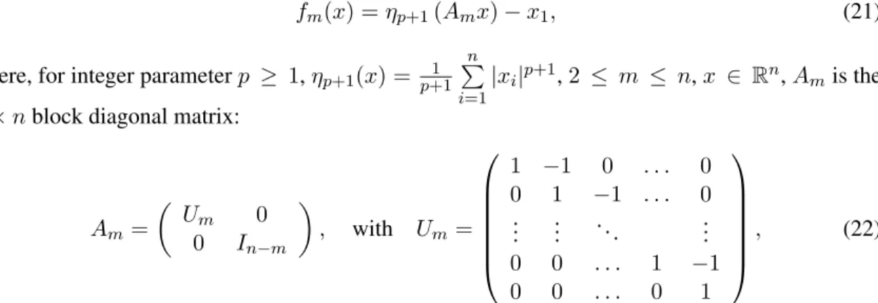
fm(x) =ηp+1(Amx)−x1, (21)

where, for integer parameterp ≥ 1,ηp+1(x) = _p+11 n

P

i=1|

xi|p+1,2 ≤ m ≤ n,x ∈ Rn,Amis the

n×nblock diagonal matrix:

Am= Um 0 0 In−m , with Um =        1 −1 0 . . . 0 0 1 ₋1 . . . 0 ... ... ... ... 0 0 . . . 1 ₋1 0 0 . . . 0 1        , (22)

andInis the identityn×n-matrix. For a detailed description of the high-order derivatives of this class of functions, and its optimality properties seeNesterov(2018).

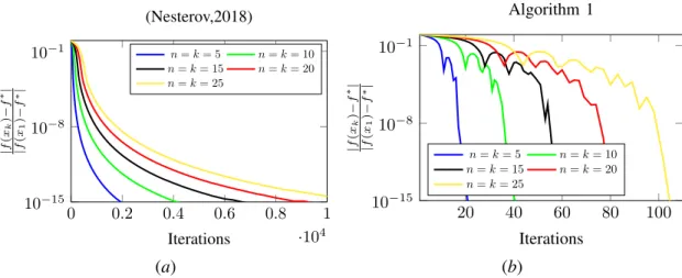
Figure1shows the normalized optimality gap of the iterations generated by the accelerated ten-sor method fromNesterov(2018) in Figure1(a), and Algorithm1in Figure1(b). We denote the min-imum function value asf∗_{. For both results we have usedp= 3, andn=k={5,10,15,20,25}.}

These numerical results show that Algorithm1requires a much smaller number of iterations than the accelerated tensor method fromNesterov(2018) to reach the same optimality gap, namely1_·10−15_,

for the class of “bad” functions described in Nesterov (2018). For example, for the case where

n = k = 25, Algorithm 1 has reached the desired accuracy in about 100 iterations, while the

0 0.2 0.4 0.6 0.8 1 ·104 10−15 10−8 10−1 Iterations | f ( xk ) − f ∗| | f ( x1 ) − f ∗| (Nesterov,2018) n=k= 5 n=k= 10 n=k= 15 n=k= 20 n=k= 25 (a) 20 40 60 80 100 10−15 10−8 10−1 Iterations | f ( xk ) − f ∗| | f ( x1 ) − f ∗| Algorithm 1 n=k= 5 n=k= 10 n=k= 15 n=k= 20 n=k= 25 (b)

Figure 1: A performance comparison between the accelerated tensor method in Nesterov(2018) (shown in (a)) and Algorithm1(shown in (b)). We minimize an instance of the family of functions in (21) withp = 3and various values of dimensionnandk. Note that thex-axis scaling on both

figures is different.

As a second set of numerical results we study the performance of the proposed method for the non-regularized logistic regression problem. For this problem we are given a set of ddata pairs

{yi, wi}for1 ≤i≤d, whereyi ∈ {1,−1}is the class label of objecti, andwi ∈Rnis the set of

features of objecti. We are interested in finding a vectorxthat solves the following optimization

problem 1 d d X i=1 ln1 + exp −yihwi, xi → min x∈Rn . (23)

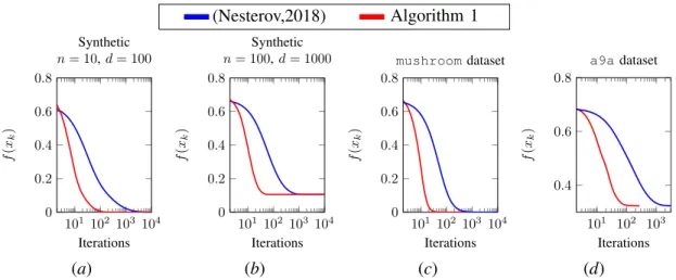
Figure 2 shows the simulation results for the logistic regression problem in (23) for various datasets. Similarly as in Figure1, we compare the performance of Algorithm 1, and the accelerated tensor method inNesterov(2018). In Figure2(a) and Figure2(b), we generate synthetic data, where, initially we define a vectorxˆ _∈ [₋1,1]with every entry is chosen uniformly at random. The set

of features for eachi, i.e.,wi ∈ [−1,1]nhas also every entry chosen uniformly at random, finally each label is computed asyi=sign(hwi,xˆi). For Figure2(a) we setn= 10andd= 100, while in Figure2(b) we setn= 100andd= 1000. Figure2(c) uses themushroomdataset (n= 8124and d= 112)Dheeru and Karra Taniskidou(2017), and Figure2(d) uses thea9adataset (n= 32561

andd= 123)Dheeru and Karra Taniskidou(2017).

For the logistic regression problem, we don’t have access to the optimal value function in gen-eral, thus, we plot only the cost function evaluated at the current iterate. As expected by the theo-retic results, Algorithm1requires one order of magnitude less iterations than the accelerated tensor method fromNesterov(2018) to achieve the same function value.

In Appendix B, we numerically compare the performance of the accelerated tensor method

(Nesterov,2018) Algorithm 1 101 ₁₀2 ₁₀3 ₁₀4 0 0.2 0.4 0.6 0.8 Iterations f ( xk ) Synthetic n= 10,d= 100 (a) 101 ₁₀2 ₁₀3 ₁₀4 0 0.2 0.4 0.6 0.8 Iterations f ( xk ) Synthetic n= 100,d= 1000 (b) 101 ₁₀2 ₁₀3₁₀4 0 0.2 0.4 0.6 0.8 Iterations f ( xk ) mushroomdataset (c) 101 ₁₀2 ₁₀3 0.4 0.6 0.8 Iterations f ( xk ) a9adataset (d)

Figure 2: Performance comparison for the non-regularized logistic regression problem between the accelerated tensor method from Nesterov (2018) and Algorithm 1. (a) Uses synthetic data with

n= 10andd= 100, (b) uses synthetic data withn= 100andd= 1000, (c) uses themushroom

dataset (d= 8124andn= 112)Dheeru and Karra Taniskidou(2017), and (d) uses thea9adataset (d= 32561andn= 123)Dheeru and Karra Taniskidou(2017).

Acknowledgments

The authors are grateful to Yurii Nesterov for fruitful discussions. The work of A. Gasnikov was supported by RFBR 18-29-03071 mk and was prepared within the framework of the HSE University Basic Research Program and funded by the Russian Academic Excellence Project ’5-100’, the work of P. Dvurechensky and E. Vorontsova was supported by RFBR 18-31-20005 mol-a-ved and the work of E. Gorbunov was supported by the grant of Russian’s President MD-1320.2018.1

References

Naman Agarwal and Elad Hazan. Lower bounds for higher-order convex optimization. In S´ebastien Bubeck, Vianney Perchet, and Philippe Rigollet, editors,Proceedings of the 31st Conference On

Learning Theory, volume 75 of Proceedings of Machine Learning Research, pages 774–792.

PMLR, 06–09 Jul 2018. URLhttp://proceedings.mlr.press/v75/agarwal18a. html.

Yossi Arjevani, Ohad Shamir, and Ron Shiff. Oracle complexity of second-order methods for smooth convex optimization. Mathematical Programming, May 2018. ISSN 1436-4646. doi: 10.

1007/s10107-018-1293-1. URLhttps://doi.org/10.1007/s10107-018-1293-1. Michel Baes. Estimate sequence methods:extensions and approximations. Technical report, 2009.

URLhttp://www.optimization-online.org/DB_FILE/2009/08/2372.pdf. E. G. Birgin, J. L. Gardenghi, J. M. Mart´ınez, S. A. Santos, and Ph. L. Toint. Worst-case

eval-uation complexity for unconstrained nonlinear optimization using high-order regularized

mod-els. Mathematical Programming, 163(1):359–368, May 2017. ISSN 1436-4646. doi: 10.1007/

S´ebastien Bubeck, Qijia Jiang, Yin Tat Lee, Yuanzhi Li, and Aaron Sidford. Near-optimal method for highly smooth convex optimization. arXiv:1812.08026, 2018.

Coralia Cartis, Nicholas I. M. Gould, and Philippe L. Toint. Improved second-order evalua-tion complexity for unconstrained nonlinear optimizaevalua-tion using high-order regularized models.

arXiv:1708.04044, 2018.

Dua Dheeru and Efi Karra Taniskidou. UCI machine learning repository, 2017. URL http: //archive.ics.uci.edu/ml.

K. H. Hoffmann and H. J. Kornstaedt. Higher-order necessary conditions in abstract mathe-matical programming. Journal of Optimization Theory and Applications, 26(4):533–568, Dec

1978. ISSN 1573-2878. doi: 10.1007/BF00933151. URLhttps://doi.org/10.1007/ BF00933151.

Bo Jiang, Haoyue Wang, and Shuzhong Zhang. An optimal high-order tensor method for convex optimization. arXiv:1812.06557, 2018.

R. Monteiro and B. Svaiter. An accelerated hybrid proximal extragradient method for convex optimization and its implications to second-order methods. SIAM Journal on Optimization,

23(2):1092–1125, 2013. doi: 10.1137/110833786. URL https://doi.org/10.1137/ 110833786.

A.S. Nemirovsky and D.B. Yudin. Problem Complexity and Method Efficiency in Optimization. J.

Wiley & Sons, New York, 1983.

Yu. Nesterov. Accelerating the cubic regularization of newton’s method on convex problems.

Mathematical Programming, 112(1):159–181, Mar 2008. ISSN 1436-4646. doi: 10.1007/

s10107-006-0089-x. URLhttps://doi.org/10.1007/s10107-006-0089-x. Yurii Nesterov. A method of solving a convex programming problem with convergence rateo(1/k2_).

Soviet Mathematics Doklady, 27(2):372–376, 1983.

Yurii Nesterov. Introductory Lectures on Convex Optimization: a basic course. Kluwer Academic

Publishers, Massachusetts, 2004.

Yurii Nesterov. Implementable tensor methods in unconstrained convex optimization. Tech-nical report, CORE UCL, 2018. URL https://alfresco.uclouvain.be/ alfresco/service/guest/streamDownload/workspace/SpacesStore/ aabc2323-0bc1-40d4-9653-1c29971e7bd8/coredp2018_05web.pdf. CORE Discussion Paper 2018/05.

Yurii Nesterov and Boris Polyak. Cubic regularization of newton method and its global perfor-mance. Mathematical Programming, 108(1):177–205, 2006. ISSN 1436-4646. doi: 10.1007/

s10107-006-0706-8. URLhttp://dx.doi.org/10.1007/s10107-006-0706-8. Andre Wibisono, Ashia C. Wilson, and Michael I. Jordan. A variational perspective on accelerated

methods in optimization. Proceedings of the National Academy of Sciences, 113(47):E7351–

Optimal Tensor Methods in Smooth Convex and

Uniformly Convex Optimization:

Supplementary Material

Lemma 5 Consider the sequence_{Ak}k≥0of non-negative numbers such that

AN ≥ 1 4 θp+12 (2R2₎pp−+11 N X k=1 A p−1 3p+1 k ! 3p+1 p+1 , (24) wherep_≥3,θ= _4(p+1)p!_M

p andMp, R >0. Then for allN ≥0we have

Ak≥ 1 cMpRp−1 k3p2+1, (25) where c= 2 3(p+1)2+4 4 (p+ 1) p! (26)

Proof We prove (25) by induction. Fork= 1we have

A1 (24) ≥ 1 4 θp+12 (2R2₎pp−+11 A p−1 p+1 1 ⇐⇒A 2 p+1 1 ≥ 1 4 θp+12 2pp−+11_R 2(p−1) p+1 ⇐⇒A1≥ p! 23p2+5(p+ 1)M_pRp−1 .

The last inequality implies (25) for p _≥ 3. Now let us assume that for allk _≤N inequality (25)

holds andN ≥1. Next we will establish (25) fork=N + 1. We have

AN+1 (24) ≥ 1 4 θp+12 (2R2₎pp−+11 N+1 X k=1 A p−1 3p+1 k !3_pp₊₁+1 ≥ 1 4 θp+12 (2R2₎pp−+11 N X k=1 A p−1 3p+1 k ! 3p+1 p+1 (25) ≥ 1₄ θ 2 p+1 (2R2₎pp−+11 1 cMpRp−1 ₃p_p−₊₁1 N X k=1 kp−21 ! 3p+1 p+1 . IfN = 1then AN+1=A2 ≥ 1 23p2+1 θp+12 (2R2₎pp−+11 1 cMpRp−1 p_p−₊₁1 (2)3p2+1. (27) IfN >1we can write AN+1 ≥ 1 4 θp+12 (2R2₎pp−+11 1 cMpRp−1 p_p−₊₁1 1 + N X k=2 kp−21 ! 3p+1 p+1 . (28)

Since p−1

2 ≥1the functionf(x) =xis convex and, as a consequence, we get

N X k=2 kp−21 ≥ N Z 1 xp−21dx= 2 p+ 1N p+1 2 − 2 p+ 1 ≥ 2 p+ 1N p+1 2 −1 2. (29)

Using this fact we continue:

AN+1 (29) ≥ 1 4 θp+12 (2R2₎pp−+11 1 cMpRp−1 p_p−₊₁1 1 2 +N p+1 2 3_pp₊₁+1 ≥ 1 4 θp+12 (2R2₎pp−+11 1 cMpRp−1 p_p−₊₁1 N3p2+1.

For allN >1we have

N N + 1 3p₂+1 = 1₋ 1 N + 1 3p₂+1 ≥ 1₋ 1 2 3p₂+1 = 1 23p2+1 .

From this and (28) we obtain that for allN _≥1

AN+1 ≥ 1 23p2+1 θp+12 (2R2₎pp−+11 1 cMpRp−1 p−1 p+1 (N + 1)3p2+1.

It remains to show that (26) implies

1 23p2+1 θp+12 (2R2₎pp−+11 1 cMpRp−1 p_p−₊₁1 = 1 cMpRp−1 . Usingθ= _4(p+1)p!_M p we get 1 23p2+1 θp+12 (2R2₎pp−+11 1 cMpRp−1 p_p−₊₁1 = 1 cMpRp−1 ⇐⇒ cp+12 1 23p2+1 p! 4(p+ 1) _p+12 1 2pp−+11 = 1 ⇐⇒cp+12 = 2 3p+1 2 4(p+ 1) p! _p+12 2pp−+11 ⇐⇒c= 2 (3p+1)(p+1) 4 4(p+ 1) p! 2 p−1 2 ⇐⇒c= 2 3(p+1)2+4 4 (p+ 1) p! ,

which is exactly what we have in (26).

Appendix B. Comparison of the accelerated tensor method fromNesterov(2018) for

p= 2andp= 3.

In this appendix, we numerically compare the performance of the accelerated tensor method pro-posed in (Nesterov, 2018), for p = 2 and p = 3. We also compare the accelerated and

10

20

30

40

50

0

.

8

0

.

85

0

.

9

0

.

95

1

Iterations

f

(

x

)

in (21),

m

= 50

,

n

= 100

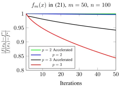
Figure 3: Performance of tensor methods and accelerated tensor methods for p = 2 andp = 3

on a difficult instance (21) for all unconstrained minimization tensor methods withn = 100and m= 50.

Similarly as in Figure 1 and Figure 2, we present the numerical results for the class of bad functions defined in (21) and one instance of the logistic regression problem.

In Figure 3, we compare the behavior of the following methods: 1) tensor method Nesterov

(2018) for p = 3; 2) accelerated tensor method Nesterov (2018) for p = 3; 3) tensor method

Nesterov(2018) forp = 2; 4) accelerated tensor method Nesterov(2018) forp = 2. Again, the

optimal function value is denoted byf∗. Interestingly, we obtain that the non-accelerated method

outperforms the accelerated method for the first m iterations. Since Theorem 4 from Nesterov

(2018) works only fork _≤ mwe don’t study the behaviour of the methods for larger number of

iterations. Even in this simple setting it is still non-trivial how to implement tensor methods for such bad examples of functions.

20 40 60 80 100 0.4 0.6 0.8 Iterations f ( xk ) Covertype dataset p= 2Accelerated p= 3Accelerated p= 2 p= 3

Figure 4: Function value achieved by the iterates of the accelerated tensor method for the logistic regression problem on theCovertypedatasetDheeru and Karra Taniskidou(2017). Number of samplesd= 20000, dimensionn= 55.

In Figure4, we consider the behaviour of the same set of methods as in Figure3, but for logistic regression problem defined in (23) on Covertype datasetDheeru and Karra Taniskidou(2017). And again, we notice that in both cases non-accelerated version works better in our experiments

First of all, we point out that tensor methods in general are non-trivial in implementation, so, it is interesting direction of the future work to get better implementation. Secondly, we conjecture that slow convergence that we see in our experiments is because of largeMp that we use. Due to tuning of the parameters one can obtain better convergence in practice.