Machine Learning for Network
Automation: Overview, Architecture,
and Applications [Invited Tutorial]
Danish Rafique
and Luis Velasco
Abstract—Networks are complex interacting systems involving cloud operations, core and metro transport, and mobile connectivity all the way to video streaming and similar user applications. With localized and highly en-gineered operational tools, it is typical of these networks to take days to weeks for any changes, upgrades, or service deployments to take effect. Machine learning, a sub-domain of artificial intelligence, is highly suitable for complex system representation. In this tutorial paper, we review several machine learning concepts tailored to the optical networking industry and discuss algorithm choices, data and model management strategies, and integration into existing network control and management tools. We then describe four networking case studies in detail, covering predictive maintenance, virtual network topology manage-ment, capacity optimization, and optical spectral analysis.
Index Terms—Analytics; Artificial intelligence; Autono-mous networking; Big data; Communication networks; Machine learning; Optical fiber communication; Telemetry.
I. I
NTRODUCTIONO
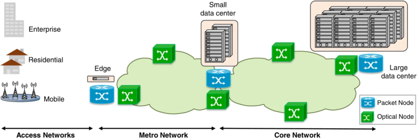
ptical communication networks may very well be regarded as the cornerstone of modern society. Internet-based applications and classical enterprise facili-ties both rely on a complex mesh of optical networking in-frastructure to address connectivity requirements. In order to support such differentiated service offerings, optical net-works have incorporated a series of innovations over recent decades, including the development of lasers, amplifiers, fibers, coherent detection, and digital signal processing, to name a few. With recent advances in mobile communi-cation systems—5G networking [1], together with exten-sive service-oriented cloud platforms like Uber, Amazon, etc.—optical transport stakeholders face tremendous challenges in terms of harmonizing stagnating revenue streams and growing networking demands [2,3].The industry has traditionally relied on hardware-centric innovations and continues to do so successfully— for instance, via photonic integration, graphene, space division multiplexing, etc. Figure1depicts a typical
archi-tecture of a multi-domain optical network, encompassing core, metro, and access networks. The various network seg-ments typically need to work together to support multi-layer services and applications, either directly or through a hybrid wireless/wireline infrastructure. This diverse, dynamic, and complex mesh of networking stacks, together with future mobility constraints, necessitates smart and end-to-end service-oriented software frameworks to aug-ment conventional hardware advanceaug-ments. To this end, software-defined networking (SDN)-triggered control and orchestration has been introduced in the past few years, allowing for separation of control and data planes in vari-ous degrees of centralization [4,5]. Furthermore, network function virtualization (NFV) has been used in tandem to abstract physical device functionalities. The challenge, however, is that of augmenting network management and control tools with adaptive learning and decision-making across multi-layer and multi-domain network architectures in a cost- and energy- efficient manner, facili-tating end-to-end network automation.
Artificial intelligence (AI) is the science of creating intel-ligent machines capable of autonomously making decisions based on their perceived environment [6]. Machine learn-ing (ML), a branch of AI, enables this learnlearn-ing paradigm (see [7,8]). ML may be used to achieve network-domain goals ranging from laser characterization [9] to erbium-doped fiber amplifier (EDFA) equalization [10], predictive maintenance [11], and failure localization [12,13], as well as related capital expenditure (CAPEX) and operational expenditure (OPEX) savings. ML algorithms are character-ized by a unique ability to learn system behavior from past data and estimate future responses based on the learned system model. For a comprehensive survey of AI methods in optical networks, we refer the reader to [14,15].
With recent improvements in computational hardware and parallel computing, such as the commercialization of big data monitoring, storage, and processing frameworks, maturity of ML algorithms, and introduction of SDN/NFV platforms, several optical networking challenges may be partially or fully addressed using ML paradigms. The key motivations together with underlying application sce-narios are listed below:
–Heterogeneity: Optical networks are a diverse and dynamic medium. Service allocations, transmission performance, optimum configurations, etc. continuously evolve over https://doi.org/10.1364/JOCN.10.00D126
Manuscript received March 28, 2018; revised June 30, 2018; accepted June 30, 2018; published August 23, 2018 (Doc. ID 327126).
D. Rafique (e-mail: [email protected]) is with ADVA Optical Networking SE, Fraunhoeferstr. 9a, 82152 Munich, Germany.
L. Velasco is with Universitat Politecnica de Catalunya, 08034 Barcelona, Spain.
1943-0620/18/10D126-18 Journal © 2018 Optical Society of America
© 2018 Optical Society of America. Users may use, reuse, and build upon the article, or use the article for text or data mining, so long
as such uses are for non-commercial purposes and appropriate attribution is maintained. All other rights are reserved.
time. While traditionally these were handled based on static design principles, this approach no longer scales owing to differentiated and often contrasting service and operational requirements.
–Reliability: Optical communication infrastructure is typi-cally built to last. This is achieved via fail-safe designs, incorporating various engineering and operational mar-gins, etc. While this approach worked well for traditional network design and operation, the scale, complexity, and sheer combinations of equipment types, part numbers, soft-ware releases, etc., especially in the context of open line systems (OLS), render this approach practically infeasible. –Capacity: Link and network capacity throughout optimi-zation is a typical metric of network design. In fact, it is one of the most important features in terms of a solu-tion’s commercial viability. A typical differentiator in ser-vice-provider-issued requests for proposals is if a certain configuration can achieve a particular optical reach with high spectral efficiency. Conventionally, precise engineer-ing rules are devised in order to fulfill such tasks. However, the number of configurations supported by the upcoming generation of optical transceivers does not play well with this approach.
–Complexity: Optical networks are often built in compli-cated meshed architectures. In several scenarios, opti-mum principles are either difficult to model (e.g., network planning), or it is impossible to come up with closed-form analytical models or fast heuristics. This leads to severe under-utilization of system resources, resulting in both OPEX and CAPEX overheads. –Quality Assurance: With growing complexity, the task of
network testing and verification is becoming increasingly prohibitive. Network operators are neither comfortable nor ready to deploy live traffic on untested configura-tions, and the concepts of self-optimization are highly suited for such problems.
–Data Aspects: An optical network is a sensor pool in itself, with data ranging from service configurations to mainte-nance logs. Most of this treasure is largely untapped in commercial systems. Discovering known and unknown patterns in a network allowing intelligent and autono-mous operations can lead to a wealth of optimization
possibilities. Here, ML can help to abstract various functionalities, enabling data-driven tasks with limited manual interventions and/or interruptions.
Despite the promise and scale of ML paradigms, the goal of learning-based optimization—considering the extent of services, infrastructure, and operational requirements—is extremely challenging. A few realistic challenges are listed below:
–There exists no blueprint for how to design and operate learning-based networks at scale. While ML promises self-regulated autonomous operation, exploiting and modeling intrinsic network complexities, its fundamen-tal advantages are far from clear.
–ML has been successfully used in several domains, and the choice of data, algorithms, architectures, etc. are somewhat clear for problems such as image recognition. However, the selection, complexity, and optimization of ML algorithms for optical networking problems requires substantial research efforts.
–Typically, ML requires huge amounts of data. How such data can be collected, processed (e.g., denoising, sam-pling, etc.), and transferred is an open problem. –The concept of ML in networking is a layer
multi-domain problem, involving several entities and stake-holders. Furthermore, the toolchain to integrate ML frameworks with network orchestration and SDN/NFV at scale is missing, and substantial work needs to be done on network control, management integration, and evalu-ation efforts.
While addressing all these facets is an enormous under-taking, in this tutorial, we take the initial steps towards this overall objective and introduce the major concepts and applications of ML in optical networking. In Section II
we introduce various aspects of ML, including the general framework, algorithms, and evaluation techniques. We follow this up with data management considerations in Section III and highlight relevant challenges. Section IV
introduces network management architectures incorporat-ing ML-driven buildincorporat-ing blocks for network automation. In SectionVwe propose several ML use cases, together with Residential Enterprise Mobile Small data center Metro Network Edge Access Networks Large data center Core Network Packet Node Optical Node
concrete real-world studies. Finally, SectionsVIandVIIgive an outlook for furthering ML research in optical networking and draw conclusions, respectively.
II. M
ACHINEL
EARNINGA. Introduction and Workflow
ML is typically thought of as a universal toolbox, ready to be used forclassificationproblems, identifying a suitable cat-egory for a new set of observations, andregressiontasks, es-timating the relationship among given data samples. In fact, it is a diverse field comprised of various constituents and necessitates: a software ecosystem including data monitoring and transformation, model selection and optimization, perfor-mance evaluation, visualization, and model integration, to name a few. Explicitly, ML refers to computational represen-tation of a phenomenon aimed at execution of a task, given a certain performance and based on a given environment.
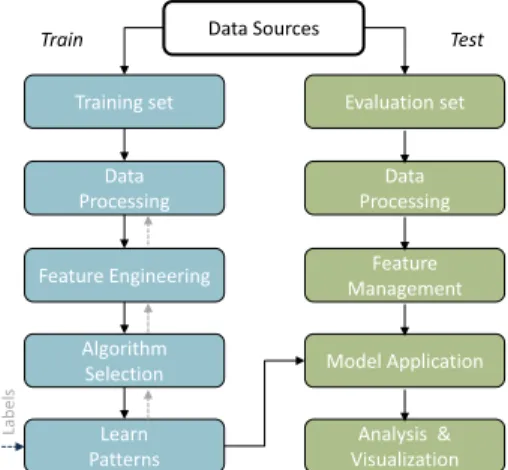
Figure2depicts a typical workflow of a ML framework— sometimes referred to as knowledge discovery in databases (KDD)—focusing on algorithm development and test cycle. Initially, ML models are constructed in atraining phase, where data is retrieved from historical databases and pre-processed to remove or normalize outliers, handle missing data, filter and aggregate parameters, etc. The next step relates to data transformation, selecting relevant data features, minimizing redundancies, data format adap-tation to the given task, etc. This is a crucial step in the ML workflow, as not all data at hand is necessarily useful in terms of algorithm performance and complexity—the curse of dimensionality. The most important steps of model selection and behavior learning are typically carried out in tandem. The process involves high-dimensional parameter optimizations and corresponding evaluations to trade off performance, complexity, and computational effort. Typically, some data is sampled from the original data set, termed as validation data, and is used together with the training data to independently verify the rules and patterns constructed in trained models. The goal of the validation stage is to ensure that ML models are not over- or underfitting the ob-served data. Note that, depending on the ML family, labeled
data may or may not be required (see the next section for further details). Finally, the models are exposed to test data, outcomes are mapped to representative knowledge (e.g., a particular pattern), and insights are delivered either to a dashboard or other related software components. Note that the presented workflow represents a typical procedure; how-ever, practical constraints may enforce a different order or amalgamation of some steps, among other variations.
B. Algorithms
ML approaches may be categorized based on objectives of the learning task, where these objectives may target pattern identification for classification and prediction, learning for action, or inductive learning methods. The algorithms may be further classified into three distinct learning fami-lies [16], i.e., supervised learning, unsupervised learning, and reinforcement learning. Semi-supervised learning—or hybrid learning—is sometimes considered a fourth branch, borrowing features from the supervised and unsupervised categories [17].
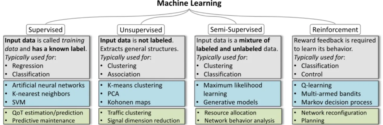
In this subsection, we introduce the ML families, as de-picted in Fig.3. The main goal is to introduce the reader to typical ML algorithms, together with their most commonly associated applications, e.g., predictive maintenance based on supervised learning [18]. Note that the list of algorithms is not exhaustive and the interested reader can find many other algorithms in the references provided.
(i) Supervised Learning: Supervised learning (SL) makes use of known output feature(s), named labels, to derive a computational relationship between input and output data. An algorithm iteratively constructs a ML model by updating its weights, based on the mapping of a set of inputs to their corresponding output features. SL may be further catego-rized into classification and regression tasks, depending on whether discrete or continuous output features are used. In the following, we discuss a few SL algorithms [19]. 1) K-Nearest Neighbors: A non-parametric ML algorithm
based on dissimilarity between the samples. For classi-fication problems, suppose there are n samples, X1,Y1,X2,Y2,…,Xn,Yn in space Rd, where X andY represent input samples and their class labels, respectively. For a new data pointX,Y, using a dis-tance measurement, all the samples would be ordered by the distances, e.g.,jX1−Xj≤…≤jXn−Xj. The class
that owns the most samples among thek-nearest sam-ples ofX, wherekis a user-defined parameter, is con-sidered the class of the new data point. In a regression application, the algorithm is used to predict the value of a continuous variable, where the predicted outcome is the average or weighted-distance average of the k-nearest neighbors.
2) Artificial Neural Networks (ANN): A ML approach com-prised of one input and one output layer and one or more hidden layers in between, where each layer could be composed of several neurons [20]. Features (X) are fed into the network through the input layer, where the neurons in the input layer are connected with the Fig. 2. Machine learning model construction and test workflow.
neurons in the next layer, i.e., the first hidden layer, and so on. The neurons on the output layer are directly con-nected with the outputs (Y), as shown in Fig.4. In a typical fully connected ANN, the nonlinear mapping between layers could be given by reluX×Wb, where Wrepresents the weights,brepresents the biases of the connections, and relu is the activation function, max0,x. Further ANN parameter optimizations are carried out using algorithms like gradient descent, etc. Other types of neural networks include convolutional neural net-works, recurrent neural netnet-works, etc. Typical challenges associated with ANNs relate to choice of number of hid-den layers and neurons, computational overhead, multi-dimensional parameter optimizations, etc.
3) Support Vector Machine (SVM): A classification tech-nique targeted at separating samples of different classes in a given feature space. The space is divided by maxi-mizing margins (i.e., gaps) between the classes, where new data points are classified based on which side of the gaps they fall on. SVMs could be categorized into lin-ear and nonlinlin-ear SVMs. For linlin-ear SVMs, the inputs are linearly transformed, whereas in the nonlinear case, the inputs are transformed into another space by a kernel mapping. A common kernel mapping is the Gaussian
radial basis function,kxi,xj exp−γjxi−xjj2, where
γ>0, andxi andxj are two samples.
The algorithm is also classified by soft and hard mar-gins. In a binary classification case, the margins are considered hard when they are represented by 1 and
−1. When the loss function max0, 1−yiω×xi−b is maximized, the margins are considered as soft. Optical networking applications of SL algorithms in-clude resource optimization by estimation and eventual prediction of network state parameters for a given set of configurations (e.g., symbol rates, optimum launch power, etc.) [21]. Another application is ML-driven fault iden-tification, based on historical traffic or network function patterns [11].
(ii) Unsupervised Learning: While SL provides a clean-slate approach to ML model construction, in practice, labeled data is neither easily accessible nor abundantly available. Unsupervised learning (USL) aims to build rep-resentation of a given data set without any label-driven feedback mechanisms. USL may be further classified into clustering of data into similar groups, or association rule discovery, identifying relationships among features. A few USL algorithms are discussed below.
1) K-Mean Clustering: An unsupervised ML algorithm, which partitions all of the samples intokclusters based on dissimilarity metrics. Considering n samples in spaceRd,X
1,Y1,X2,Y2,…,Xn,Yn,k-mean cluster-ing tries to cluster all the n samples into k classes, centered by the setSS1,S2,…,Sk. The objective
func-tion could be defined as arg max S Pk i1 P x∈Sijx−μij 2,
whereμiis the mean of all the points inSi.
2) Principal Component Analysis (PCA): Transforms the original variables into linear uncorrelated variables based on singular value/eigenvalue decomposition. Typically used as a dimension reduction approach. Consider a data matrix X, with zero-mean columns, where each row in X represents one observation and each column represents a single attribute. PCA trans-formation aims to reduce the data matrixXfromn di-mensions intopdimensions by multiplying a weights matrix W w1,…,wp, where W is obtained by the Fig. 3. ML families. The first box in each column identifies the main characterization of the ML approach; the second box identifies ex-amples of algorithms used in the approach; and the third box indicates exex-amples of applications that can take advantage of the approach.
objective function arg maxWTXTXW. The value ofXTX is the largest eigenvalue ofX, andWis the correspond-ing eigenvector ofX.
3) Self-Organizing Maps (SOM): This is a method for di-mensionality reduction, where an ANN (the map) is trained using unsupervised learning to approximate samples in a high dimensional space. Typical use in-cludes feature identification in large datasets. In the training phase, the weights within the network are up-dated by competitive learning, described by the pseudo-code in Algorithm 1.sis the current iteration number, tis the index of the target input data vector in the input data setD,Dtis a target input data vector,vis the index of the node in the map,Wvis the current weight vector of nodev,uis the index of the best matching unit (BMU) in the map,θu,v,sis a penalizing parameter based on the distance from the BMU, andαsis a learn-ing coefficient.
Algorithm 1:SOM
1: Randomize the node weight vectors in a map 2:repeat(for eachepisode)
3: Randomly pick an input vectorDt 4: repeat(for eachnode in the map)
5: Use the Euclidean distance formula to find the 6: similarity between the input vector and 7: the node’s weight vector
8: Track the node with the smallest distance 9: (termed as the best matching unit, BMU) 10: untilall the nodes are traversed
11: Update the weight vectors of the nodes 12: (in the neighborhood of the BMU) 13: by pulling them closer to the input vector 14: Wvs1 Wvs θu,v,s·αs·Dt−Wvs 15:untilsis terminal
USL models may be naturally used for clustering of transport channels, nodes, or devices, based on their tem-poral and spatial similarities. Applications include traffic migration, spectral slot identification, etc. (see, e.g., [22]).
(iii) Reinforcement Learning: Reinforcement learning (RL) refers to ML mechanisms without an explicit training phase [23]. RL aims to build and update a ML model based on an agent’s interaction with its own environment. The key difference with respect to SL techniques is that labeled input–output features are not provided, but the relation-ship is rather learned via application of the initial model to test data. The most well-known reinforcement learning technique isQ-learning [24], described below.
1) Q-Learning: This algorithm tries to find the best poli-cies under specific agent and environmentalQvalues. The basic elements of Q-Learning include states Ss1,s2,…,snand actions Aa1,a2,…,am. A policy
πis a rule chosen by the agent, and it consists ofsi,aj, where at statesi, actionajis executed. The agent choo-ses policies based on the value functionQs,a. The pseudo-code forQ-learning is shown in Algorithm 2. Here,rmeans rewards, which are defined by the agent,γis
a discount factor, andαis the learning rate. Theε-greedy policy means that with a given probabilityε, the agent will choose a random action; otherwise, it will choose the action with maximalQ value.
Algorithm 2:Q-Learning 1: InitializeQs,aarbitrarily 2: repeat(for eachepisode) 3: Initializes
4: repeat(for eachstep of episode) 5: Chooseafromsusing policy derived 6: fromQ(e.g.,ϵ- greedy)
7: Take actiona, observer,s0
8: Qs,a←Qs,aαrγmaxa0Qs0,a0−Qs,a
9: s←s0
10: untilsis terminal 11: until end episodes
One of the core applications of RL algorithms in optical networks is network self-configuration, including resource allocation and service (re)configurations—both for physical and virtual infrastructure (see, e.g., [25]). Network man-agement frameworks may be extended with RL to come up with cognitive actions.
C. Evaluations
The ML algorithm evaluation approach impacts the way a model is constructed and eventually selected among several competing options. A poorly defined evaluation criterion may result in an unoptimized model selection procedure, resulting in erroneous conclusions when com-paring classifier performances. The key questions to be answered are how to build models, how to meaningfully evaluate their performances, and how to determine the best configurations. In this subsection we focus on the data and performance aspects of ML model construction and introduce several evaluation strategies.
(i) Data Aspects: The fundamental aspect of building a ML model is to separate the available data set into train-ing, validation, and test sets. The training data is used to build the model, whereas the validation set is used to inde-pendently validate the model constructed during the train-ing phase. Finally, the test data, which is never observed by the model during its construction process, is used for per-formance evaluations.
The reason to divide data into these sets is to avoid over-fitting the training data as depicted in Fig.5. It can be seen that as the model approaches convergence—underfitting, which refers to an overly simplistic model—the training and validation data sets show similar results; however, beyond this phase, training errors continue to improve, whereas validation errors start deteriorating—overfitting, which refers to an unnecessarily complex model. The model that enables the best performance for the validation set is selected as the optimum model. Based on data character-istics, various cross-validation approaches may be used to split the training and validation set for model construction. For instance,k-fold cross-validation includes splitting the
data set intokseparate sub-sets—as shown in Fig.6—then training fromk−1 sub-sets, evaluating the remaining set, and repeating the procedure until all sub-sets are covered. Finally, the error metrics from each iteration are averaged to give overall performance estimation. Typically,kis set to 5 or 10 but may also take other values.
Another caveat is class imbalance, a common problem in a wide range of ML application areas. This problem usually appears in the form of dominant negative outcomes and may be partially resolved via data re-sampling methods.
(ii) Performance Aspects: There exist several evaluation techniques suited to a diverse set of ML models. For the sake
of simplicity, let us assume a two-class classifier, where the classes represent a set of positive and negative outcomes. –Confusion matrix: TableIlists the most common
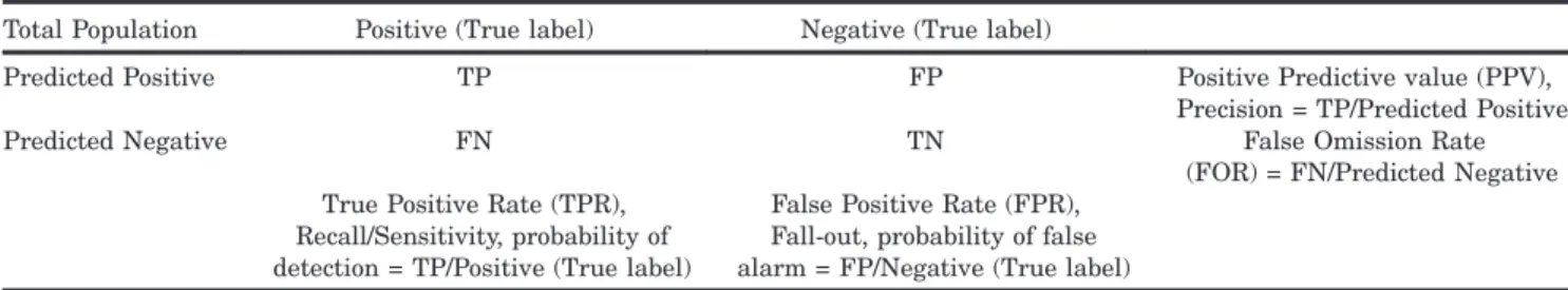
evalu-ation factors, i.e., true negative (TN), false negative (FN), false positive (FP), and true negative (TN). Such tabular representation is typically used as an evaluation approach for binary classifiers. The individual metrics are then used to calculate various sub-metrics.
–Sensitivity or True positive rate (TPR): TPRTP∕TP FN and gives the probability that a true outcome is actually true.
–Specificity (SPC) or True negative rate: SPCTN∕ TNFPand gives the probability that a false outcome is actually false.
–Precision or Positive predictive value (PPV): PPV TP∕TPFPand refers to the proportion of true out-comes given a set of outout-comes classified as true. –False omission rate (FOR): FORFN∕FNTN and
refers to the proportion of false negatives given a set of outcomes classified as false.
–ROC and AUC: The receiver operating characteristic (ROC) curve is obtained by plotting TPR as a function of FPR and varying the class decision thresholds. An ideal classifier would entirely separate the two classes, resulting in a ROC curve that passes through the top left (100% sensitivity and specificity), as shown in Fig.7. Fig. 5. Underfitting versus overfitting.
Fig. 6. k-fold cross-validation.
TABLE I
CONFUSIONMATRIX FOR ABINARYCLASSIFIER Total Population Positive (True label) Negative (True label)
Predicted Positive TP FP Positive Predictive value (PPV),
Precision = TP/Predicted Positive
Predicted Negative FN TN False Omission Rate
(FOR) = FN/Predicted Negative True Positive Rate (TPR),
Recall/Sensitivity, probability of detection = TP/Positive (True label)
False Positive Rate (FPR), Fall-out, probability of false alarm = FP/Negative (True label)
Fig. 7. ROC- and AUC-based classifier evaluation. The dotted and dashed lines are examples of typical ROC curves; the classifier corresponding to the dashed line provides better performance.
The area under the curve (AUC) is the area under the ROC curve, and it represents the precise quality of the binary classifier, regardless of the decision threshold.
In the case of multi-class problems, binary classification approaches may not be used to evaluate performance. Below we describe several evaluation metrics, whereyrepresents true values,yˆrepresents predicted values, andy¯depicts the average of the true values. The erroreis obtained byy−yˆ. –Accuracy: The rate of correct predictions made by the model over a test data set, typically via simple network management protocol.
–MAE and MAPE: Mean absolute error, meanjej, and mean absolute percentage error, mean100 × abse∕y. –MSE: Mean square error, meane2.
–R2: The ratio between predicted variation and true
var-iations, R2SSE∕SST, where SSTP
iyi−y¯2, and SSEPiyi−yiˆ 2. It indicates how close the predicted values are to the real values.
Note that the presented techniques are not exhaustive by any means but rather an introduction to standard evalu-ation measures. There are several other approaches pre-sented in the literature and are typically used based on the data and the problem at hand.
III. DATA
MANAGEMENT
An optical network generates a large amount of hetero-geneous data streams, which must be fetched, processed, and analyzed in a timely manner to enable everyday net-work operations. In order to enable data-driven ML analy-sis, it is important to explore several aspects of network data including its extent, monitoring, query mechanisms, storage, and representation attributes. In this section, we address these data management features.
A. Sources
The first step in enabling ML-driven network operations is to understand the variety of network data sources, ranging from physical layer channel information all the way to applications and services. In the following, we dis-cuss the five most common sources of ON data collection. –Network probesinclude both intrusive and non-intrusive data access, e.g., measured optical power at an oscillo-scope and deep packet inspection for filtering packets or collecting statistics, respectively.
–Sensors are the core data sources of optical networks, whose goal is to measure a physical quantity (device, sub-systems, sub-systems, and environment). These sensors may be explicit, e.g., a temperature measure, or implicit to network equipment, e.g., timing error. Typical examples of sensor data include received bit error rate, aggregate traffic rate, virtual network function (VNF) flow informa-tion, amplifier gain, etc.
–Network logs include alarm and event data sets from different network devices. Service and support teams
examine these logs to initiate network diagnosis and action recommendations.
–Control signaling refers to supervisory channel, header data, etc., typically used for path initialization, link con-trol, channel setup, etc.
–Network management datais primarily focused on two types of data sources: first, configuration, topology, and connectivity data at different network layers, and second, monitored data (typically via simple network management protocol [SNMP] MIBs) [26] obtained from the network sensors described above.
The network data may be further categorized based on their type and form, as given below.
–Static datarefers to condition monitoring at a given time instant and may include both performance and configu-ration data.
–Dynamic data refers to time variable quantitative parameters, for instance, temperature, packet loss rate, received and transmit power levels, etc.
–Text data includes log files, manuals, design specifica-tions, device models, etc.
–Multi-dimensional datatypically represents image data, including device snapshots, locations, etc.
TableIIlists several optical network data variables and their corresponding device, subsystem, and system. Note that here we exclusively focus on network data metrics, excluding end-user information like transmission control protocol, user datagram protocol, etc. Different subsets of presented variables may be used for different ML use cases. For instance, optical signal-to-noise ratio (OSNR), bit error rate (BER), and optical power may be used for physical layer performance optimization, whereas packet count, traffic load, and flow count may be used for network reconfiguration applications.
B. Monitoring
Network monitoring comprises accessing the aforemen-tioned diverse data types. The challenge, however, is that the network devices are typically provided by a diverse set of equipment suppliers with unique interfaces, models, descriptions, etc. Moreover, the traffic itself is extremely heterogeneous with different formats, wavelength ranges, etc. Consequently, next-generation networks will represent a wide variety of rapidly evolving application stacks, con-suming both physical and virtual resources. Traditional network management tools are unable to efficiently tap into this data goldmine because they lack the capabilities to probe network states in real time, among other issues related to scalability, vendor lock-in, etc. For instance, SNMP-based monitoring largely relies on data access at fixed intervals, managed using trap-based alarms. While SNMP has served the industry long and well, network monitoring needs to rise to the new visibility requirements. On the other hand, model-driven streaming telemetry is defined by operational needs and requirements set by
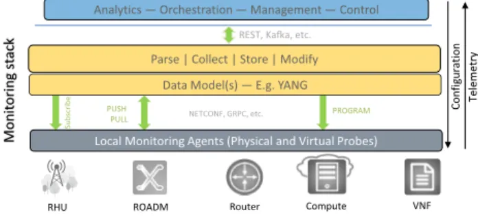
telecom network operators (e.g., OpenConfig, TAPI). Figure8 illustrates the core components of model-driven telemetry. It enables vendor-agnostic network state moni-toring on a continuous basis using time series data streams and abstracts data modeling from data transport [27], lev-eraging advanced open-source initiatives, like YANG— model—, Google remote procedure call (GRPC)—transport, etc. Note that the northbound and southbound communi-cation incorporates data and configuration exchange, e.g., to transport data to an SDN controller, and triggered configuration from the same controller. Furthermore, one of the key differentiators in moving from legacy mon-itoring (e.g., SNMP) to model-driven telemetry is the use of subscription-based data access, as opposed to request- or trap-based desired data selection and retrieval.
Table III lists a few key differences between legacy SNMP and state-of-the-art streaming telemetry solutions. On one hand, most telemetry solutions are based on participation-based standards organizations, whereas GRPC follows its own open-source development structure. The key differences arise from the multi-vendor operability and scale of the projects, e.g., sFlow being a generalized sol-ution, compared to GRPC focusing on the management and control planes, etc.
C. Data Storage and Representation
Having discussed data sources and access mechanisms, data storage and representation also play an important part in data management frameworks. Due to the growing size of the network and complexity of the information sources, the data sources are often scattered across multi-ple storage and management systems with their own pecu-liar features. For example, there are storage technologies such as relational databases that require a dedicated data model or schema, whereas non-structured query lan-guage (NoSQL) databases serve the purpose without any relational model and have better scalability. However, both these technologies often fail when the volume and complexity of data becomes tremendously large. Recent advancements have demonstrated the utility of big-data technologies; for example, using Hadoop clusters, Spark, or Teradata to store and process huge amounts of data in a distributed fashion.
Nonetheless, it is not unusual for a typical network infra-structure to have its data scattered over these different heterogeneous data sources or systems that have been adapted over time to fulfill the requirements of the applica-tion they serve. This often leads to situaapplica-tions where data retrieval becomes a bottleneck due to the different represen-tation schemes, constraints, naming conventions of the schema elements, formats used within the data models, etc. Fig. 8. Model-driven telemetry stack. REST, representational state
transfer; RHU, remote hub unit; VNF, virtual network function.
TABLE III
LEGACYVERSUSMODEL-DRIVENNETWORKTELEMETRY
Technology SNMP sFlow NETCONF GRPC
Models MIBs Structures YANG YANG
Transport UDP UDP SSH HTTP
Encoding ASN.1 XDR XML GPB
Standard IETF sFlow IETF –
Type Pull Push Push Push
Application Generic Generic Large-scale Large-scale TABLE II
EXAMPLES OFOPTICALNETWORKDATASOURCES
Parameter Transmitter Receiver Amplifier ROADM NMS Scope Shelf Switch
Optical power X X X X BER X OSNR X X X X X Amplifier gain X Fiber type X Distance X Line rate X X X Client rate X X X Pluggable type X Traffic load X X Temperature X X X X X X
Main supply voltage X
Frequency resolution X
Flow count X
Packet count X
Topology X
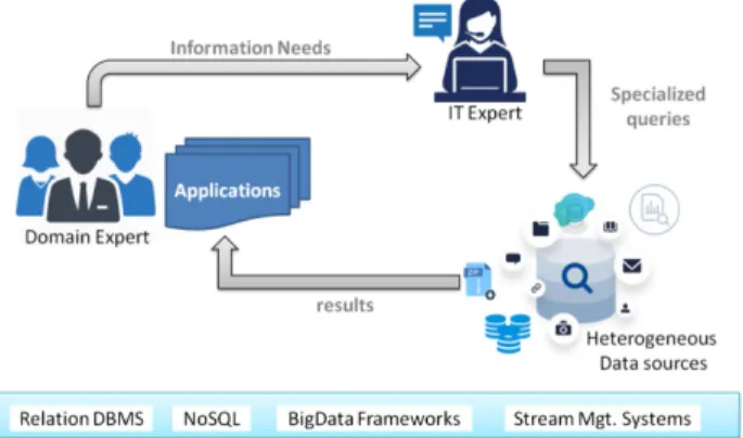
Most enterprises today have dedicated teams of IT spe-cialists to develop database queries for the domain experts. This means that the domain experts always have to pass their information needs to IT specialists (see Fig.9), and this can drastically affect the efficiency of finding the right data in the right format that can be used for timely decision-making. From the modeling point of view, the data model is not the same as the domain model, leading to inefficiencies in data access protocols (schema, vocabular-ies, etc.). Clearly, it would be much easier to understand, analyze, and benefit from the data if it was uniformly accessible and represented in a domain-specific language. Recently, ML and graph technologies have been adopted to create a domain-specific abstraction over the data sources and make query answering easier for experts [28].
IV. NETWORK AND
MODEL
MANAGEMENT
In order to make use of advanced ML models, these mod-els need to be integrated into the existing network software stack. On the other hand, multi-layer and multi-vendor network control and management is a complex task in it-self, involving services incorporating cloud operations, core and metro transport, and mobile front-haul and back-haul connectivity all the way to heterogeneous user applications [29]. With localized and highly engineered operational tools, it is typical of these networks to take several weeks to months for any changes, upgrades, or service deploy-ments to take effect. In this context, SDN is considered a game changer by many, owing to its agility, flexibility, and scalability, in contrast to traditional control and man-agement platforms [30]. SDN distances itself from propri-etary, device-specific operation to open, resource-driven control, enabling centralized, programmable, and auto-mated services across multiple domains. The key issue is that while SDN is progressively getting adopted in the cloud, the ecosystem around centralized SDN platforms is ossified to legacy static and hardware-centric operations. The bottleneck does not necessitate introduction of entirely new tools, but rather an upgrade of legacy technologies— service provisioning, activation, fault management, etc.
In order to attain true network automation, centralized SDN control needs to be augmented with instantaneous
data-driven decision-making using advanced monitoring and ML tools, feeding management and control planes alike. In the following we discuss the architecture of such an evolved platform.
A. Architecture
(i) Closed Loop Operation: The discussions regarding SDN have almost exclusively focused on separation of data and control planes, with little to no attention on the overall operational feedback loop, including monitoring, intelli-gence, and management functionalities. Figure10captures this theme and presents a high-level network architecture, where central offices (CO) consist of intra- and inter-data-center infrastructure. The intra-data-inter-data-center resources comprise storage, computation, and networking, whereas inter-data center connectivity is provided by a transport network. Resources—physical or virtual—are continuously monitored, exposing real-time network states to the ana-lytics stage, which in turn feeds into the control, orchestra-tion, and management (COM) system.
This holistic platform not only caters to centralized and programmable control, but also makes ML-driven deci-sions to trigger actions, essentially connecting data-driven automation with policy-based orchestration and manage-ment. To this end, the COM architecture includes the NFV orchestrator providing network services, the virtual infrastructure manager (VIM) coordinating and automat-ing data center workflows, the network orchestrator adopt-ing hierarchical control architectures with a parent SDN controller abstracting the underlying complexity, and a monitoring and data analytics (MDA) controller that collates monitoring data records from network, cloud, and applications and contains ML algorithms.
(ii) Centralized and Distributed: Regarding MDA, a hybrid architecture may be envisioned, where every CO includes a distributed MDA agent that collates monitoring data from the network, cloud, and applications as well as a centralized MDA controller [31]. The MDA agent exposes two interfaces toward the MDA controller for collection Fig. 9. Data storage and representation workflow and technologies.
of monitoring and telemetry data. In addition, specific interfaces for monitoring control allow the MDA agent to connect with the network nodes. The MDA agent includes a local module containing data analytics applications for handling and processing data records. The data analytics capabilities deployed close to the network nodes enable local control loops, i.e., localized data analysis, and conse-quent updated configurations.
The centralized MDA controller abstracts monitored data via suitable interfaces and implements a ML-based learning engine, where ML algorithms analyze monitoring data to discover patterns. Such knowledge can be used to make predictions and detect anomalies before they nega-tively impact the network. Such events can be notified in advance to the corresponding COM module (SDN con-troller or orchestrator), together with a recommended action. Note that a recommended action is a suggestion that the COM module can follow or just ignore and apply its own policies. The notification might trigger a network re-configuration, hence closing the loop and adapting the network to the new conditions.
(iii) Control Loop Examples: It is worth highlighting the importance of the control loops for network automation, as they fundamentally change the way networks are operated today—empowering truly dynamic and autonomous opera-tion. As examples of control loops, we analyze the following, in the context of the presented architecture: i) soft-failure processing and ii) autonomic virtual network topology (VNT) management.
–Soft-failure processing: Let us focus on the optical layer where lightpaths might support virtual links (vlinks) in packet-over-optical multilayer networks. Soft failures can degrade a lightpath’s quality of transmission (QoT) and in-troduce errors in the optical layer that might impact the quality of the services deployed on top of such networks. Such soft failures affecting optical signals can be detected by the MDA agents at intermediated nodes analyzing the optical spectrum acquired by local optical spectrum analyz-ers (OSA). Note that the acquired optical spectra entail large amounts of data [e.g., 6400 frequency-powerhf,pi pairs for the C-band for OSAs with 625 MHz resolution], so local analysis carried out at the MDA agents greatly re-duces the amount of data to be conveyed to the MDA con-troller. Upon detection of a soft failure, the MDA agent notifies the MDA controller, which is able to correlate notifications received from several MDA agents and for sev-eral lightpaths to localize the element that is causing the failure [13]. Once the failure has been localized, e.g., in an optical link, a notification is issued to the COM module responsible for the resources (e.g., SDN controller) together with the recommended action of re-routing the affected lightpath excluding the failed resource.
–Autonomic virtual network topology management: VNTs are commonly created to adapt demand granularity to the huge capacity of lightpaths. Because demands vary throughout the day, defining a static VNT where vlinks are dimensioned with the capacity for traffic peaks leads to huge capacity over-provisioning; thus, VNT adaptation to follow demand requirements greatly reduces costs for
network operators. One approach to dynamic manage-ment is to monitor capacity usage in the vlinks and to configure thresholds so that when a threshold is ex-ceeded, the capacity of the vlink can be (reactively) recon-figured by adding or releasing lightpaths supporting this vlink. Another option is to monitor the origin-destination (OD) and reconfigure the VNT accordingly in a proactive manner [21]. For such proactive VNT adaptation to work, OD traffic prediction is needed to anticipate demand changes. OD traffic prediction is based on fitting models using ML algorithms that use historical OD traffic data collected by the MDA agents and stored in the MDA con-troller. Those OD traffic models are also stored in the MDA controller and are ready to be used for prediction. Periodically, the SDN controller can request the pre-dicted OD traffic for the next period, e.g., the next hour, and use such prediction to create a traffic matrix that is the input of an optimization problem in charge of finding the best VNT configuration that meets both current and predicted capacity requirements.
B. ML Model Life Cycle
Once a ML model is constructed and deployed, the next step is to maintain this model over its lifetime. This process largely involves questions related to when and how a model should be updated. In particular, it is critical to determine the update cycle of a ML model considering the computational load and also ascertain the model validity while performing updates. In the following, we detail both of these aspects.
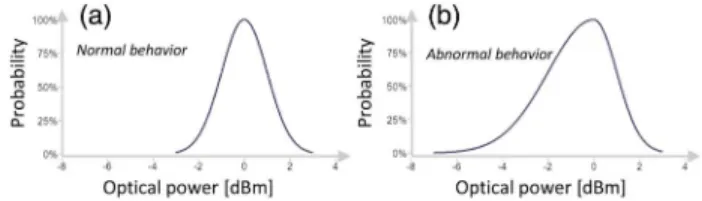
(i) Data Profile: A rather standard approach is to per-form model updates at regular intervals, termedconstant update, regularly adapting to evolving network states. While this simplifies model maintenance, it either suffers from unnecessary updates—in case network behavior has not changed significantly—or not an accurate enough model due to fast-paced changes in underlying network conditions. An orthogonal methodology is to trigger model updates when the data profile has changed significantly, termed adaptive update. This allows for efficient use of computational resources and adapts to real-time network behavior. Figure 11 shows an example of a normal and abnormal distribution for received optical power levels, triggering a model update.
(ii) Reconstruction: Model reconstruction involves incor-porating new training data into the ML model. Once a model update decision has been made, the next step is
Fig. 11. Adaptive model update based on changing data profile, as opposed to fixed duration periodic updates. (a) Normal distribu-tion of optical power levels. (b) Abnormal distribudistribu-tion of optical power levels.
to decide whether a batch-based or real-time update will be performed. Batch-based model reconstruction rebuilds the model with every refresh cycle, discarding previous data. This can be performed either in a sliding window or a weighted sliding window mode. Conversely, a real-time up-date refers to an incremental upup-date of a preexisting model based on new data. This enables computational savings by not reconstructing the entire model, where resources have already been used. Furthermore, a real-time update allows for efficient data handling, as once the model is recon-structed there is no need to store the data for future model development.
V. APPLICATION
SCENARIOS
In this section, we introduce several applications of ma-chine learning in optical networks. Broadly, we consider network failure, reconfiguration, and performance-related use cases, discuss the background and relevant prior art, and follow up with proof-of-concept demonstrations. In par-ticular, the control loop examples described in the previous section are detailed, together with two other sample appli-cations, i.e., physical layer capacity optimization and opti-cal spectrum analysis. The ML algorithms used for these applications include regression, SVM, and ANN, imple-mented using TensorFlow [32] for our proof-of-concept algorithm development.
A. Predictive Maintenance
With increasing network complexity and heterogeneity, business economics dictate the need for improved asset management to reduce, if not eliminate, downtime and improved resource usage [33]. Typical maintenance ineffi-ciencies include the following.
–Network assurance agreements are signed, requiring maintenance cycles and periodic support, without consid-ering current equipment or network health status. –Network operators need to allocate effort to monitor and
raise issues with support teams. This is typically done after a failure has occurred. Furthermore, in case of early support requests, repairs are quick fixes due to lack of a global operational perspective.
–Even in the case of data gathering and processing, most of the analysis is manual and only used for post-failure diagnostic purposes.
–The entire cycle is based on a few highly experienced individuals, with issues related to single-point-of-failure, non-transferable skills, product variations, etc.
Typical examples of network faults may include cooling unit failure, laser degradation, subsystem control unit fail-ure, etc. Early detection of equipment failure states and consequent remedial actions can prevent network down-time and enable scheduled preventive maintenance. The general functional hierarchy of a fault management system is given in Fig.12, ranging from detection of a potential failure, all the way to resolution processes [12]. Most
commercial equipment tolerates some errors until auto-matically tearing down the connection when some system thresholds are exceeded. While a restoration procedure could be initiated to recover the affected traffic, it would be desirable to anticipate such events and re-route the lightpath before it is disrupted. In case rerouting is neces-sitated, failure localization is required so as to exclude the failed resources from path computation. In addition, proac-tive failure detection would also allow time to plan the re-routing procedure, e.g., during off-peak hours.
In this use case, we address failure detection and locali-zation blocks and demonstrate an analytics-enabled fault discovery and diagnosis (FDD) architecture, capable of pro-actively detecting and localizing potential faults (anomalies) as well as determining the likely root cause—based on SDN-integrated knowledge discovery [34]. The network segment consisted of ADVA FSP 3000 modules, carrying a (moni-tored) 100 Gb/s transport service. Here we follow a two-stage fault detection approach, where, in the first stage, the opti-cal power levels are monitored as level-I data, and, in the second stage, localized level-II subscription-based monitor-ing consists of amplifier gain, shelf temperature, current draw, and internal optical power. The dual-stage approach allows for reduced monitoring and processing overhead compared to the all-at-once monitoring approach. The en-semble fault discovery and diagnosis framework is initiated within the SDN controller, as shown in Fig.13(a), eventually triggering distributed analysis [Fig.13(b)].
After initial data acquisition (aggregated in hourly bins), the algorithm is executed in two phases. In the first phase,
Fig. 12. Fault management functional hierarchy.
(a)
(b)
Fig. 13. SDN-integrated fault discovery (detection) and diagno-sis. (a) System-level FDD. (b) Node-level FDD.
the records are partitioned, and we execute the generalized extreme studentized deviation test (GESD), a sequential-processing-based modification of Grubb’s test [35], for deviation and classification tests (memory of 11 units), and neural network (backpropagation trained, in a 7(input) × 5(hidden) × 1(output) neuron configuration using tanh activation) based true fault detection. The ANN inputs re-present positive and negative fault label values (a sequence of zeros and ones), including the indicated fault identified by GESD. The role of the ANN network is to make true abnormality decisions based on these fault label patterns. The engine performs first-level layer 0 monitoring via SDN abstraction through the southbound interface (SBI). It detects potential faults and localizes them to relevant network ports. The outcome is then distributed to a net-work maintenance application (RESTful), and also to the domain controller via SBI (Netconf). Second-level func-tional blocks include local fault discovery, followed by the root cause analysis, which maps metric fault measures to available node topology and lists potential root causes in a priority log.
After first-level detection of power level anomalies (not shown for the sake of conciseness), the second-level localized analysis is triggered. Figure14(a)shows sample test points for these features, including temperature, amplifier gain, intermediate stage power, and current draw profiles, where the associated changes in a feature indicate the potential root cause. Figure14(b) shows the distance metric, based on shape-based clustering [36], amongst the probable fault root causes, identifying the response of other features with respect to each others’changes. The shorter the length along an ellipse’s minor axis, the higher the similarity between the two features; the rightwards tilt represents positive correla-tion, and vice versa. Note that the diagonal shows a line seg-ment (minor axis of length zero), representing a perfect match, as the same feature is present on both thex axis andyaxis. A high association is found between temperature and current draw as increasing temperature necessitates higher fan speed, whereas on the other hand, a decreasing
draw may increase the temperature. Furthermore, a strong anti-correlation is identified between temperature and power, followed by relatively weaker dependency between current draw and power. Power may be ruled out as a poten-tial fault because it starts deteriorating after the other two features; current and temperature are the two remaining causes, which may be processed further.
B. Autonomic Virtual Network Topology Management
Figure15(a)shows an initial VNT where every vlink is supported by a 100 Gb/s lightpath in the underlying optical layer; the MPLS path for OD 6→7 is also shown. Let us assume that a 90% capacity threshold is configured in the vlinks, and in the event of a threshold violation, the capacity of some of the vlinks is increased. In our example, as OD traffic 6→7 increases, two threshold violations—for vlinks 1→6 and 1→7—will be issued, resulting in increased VNT capacity [Fig.15(b)]. It is worth noting that the MPLS path for OD 6→7 is not affected by the VNT reconfiguration. As shown, the threshold-based reconfiguration can adapt the VNT capacity to traffic changes, such that the resources in the optical layer are allocated only when vlinks need to increase their capacity. However, the same number of tran-sponders are required as in the static VNT approach; for instance, two transponders are installed in routers 6 and 7 and another four in router 1 reserved for vlinks 1→6 and 1→7.Let us now assume that instead of monitoring vlink capacity usage, OD traffic is monitored in the nodes. By an-alyzing such monitoring data it could be observed that OD 6→7 is responsible for the registered traffic increment. In this case, let us assume that new vlinks can be created/ removed in addition to increasing the capacity of the existing ones such that the VNT is actually changed. We propose an approach where OD traffic is periodically ana-lyzed and the current VNT is reconfigured accordingly. An example that follows this approach is illustrated in Fig.15(c), where the OD traffic 6→7 is predicted for the next
(a) (b)
hour and a new vlink between nodes 6 and 7 can be created by establishing a lightpath, rerouting 6→7 traffic. Note that with this solution there are two fewer required transponders in router 1 compared to the previous approach.
(i) Proactive VNT Reconfiguration: Proactive VNT adap-tation anticipates demand changes, consequently enabling better resource management with respect to reactive strat-egies. The VNT reconfiguration problem can be defined based on traffic prediction (VENTURE) [21], which can be formally stated as the following:
Given:
•The current VNT represented by a graph GN,E0, N being the set of routers and E0⊆E the set of current vlinks. SetEis the set of all possible vlinks connecting two routers,
•the setPwith the optical transponders available in the routers; every transponder with capacityB,
•the current traffic matrixD,
•the predicted traffic matrix OD.
Output:The reconfigured VNTG⋆N,E⋆, whereE⋆⊆E, and the paths for the traffic are onG⋆.
Objective:Maximize current and predicted traffic matri-ces, while minimizing the total number of transponders used. Since we are targeting VNT adaption to current and future traffic conditions, predictive traffic models that can accurately anticipate OD traffic are needed to define traffic matrices.
(ii) OD Traffic Estimation Models: The model estimation approach that we follow here is fitting ANN models. Different ANNs need to be fitted to separately predict the bitrate of each OD traffic flow. Each ANN receives as inputpprevious data values from the monitoring data repository and returns the expected average bitrateμand the bitrate varianceσ2at timet. Other variables, like the
confidence interval at 95%, can be obtained by combiningμ andσ2 predictions.
One interesting analysis is the required training data (de-noted asY), as monitoring traffic during the right period of time is crucial to produce quality models while minimizing the time for new model availability. To evaluate this, we con-ducted experiments whereμandσ2are estimated and
evalu-ated varyingjYj. Figure15(d)shows the maximum error for
σ2 andμ estimations for different values ofjYjbetween 2
days and 3 months. Althoughμcan be estimated with less than 5% maximum error in about 10 days, a maximum error of 60% is observed forσ2for the same duration. To decrease
the maximum error,jYjneeds to be increased up to 2 months to keep maximum prediction errors under 20%.
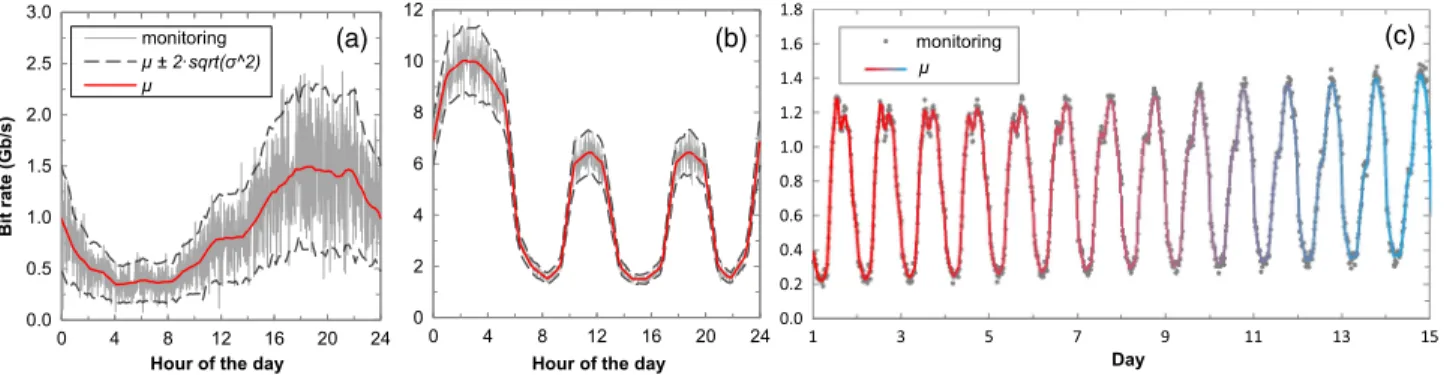
Figures16(a)and16(b)show one day of monitoring traffic data for two different traffic profiles, as well as the predic-tion of the μ model and the confidence interval at 95% obtained by combining theμandσ2models (dashed lines).
In addition, it is interesting to investigate the performance of an ANN model to smooth changes in the data. Figure16(c)
shows such adaptation to an evolutionary traffic scenario, where daily traffic pattern changes smoothly day by day. One can observe how the ANN model adapts from the initial (red) to the final (blue) traffic pattern while keeping its origi-nal accuracy without refitting.
(iii) Illustrative Results: Let us now apply the ANN traf-fic modeling approach to predict the OD bitrate of a core VNT, used as the input of the VENTURE optimization problem. Let us assume that VENTURE is triggered peri-odically, so per-OD prediction of maximum traffic for the next period is needed.
6 7 2 3 1 4 5 200 200 (a) 6 7 2 3 1 4 5 (c) 100 100 100 100 100 6 7 2 3 1 4 5 0% 20% 40% 60% 80% 100% 0 10 20 30 40 50 60 70 80 90 Days of monitoring Maximum err o r (d) (a) (b) (c)
Fig. 15. (a)–(c) Reactive and proactive adaptation. Numbers in the inset represent link capacity in gigabits per second (Gb/s). (d) Maximum prediction error versus days of monitoring.
(a) (b) (c)
For evaluation purposes, we compare the number of op-tical transponders required for static VNT management that is configured for peak traffic versus the number required with dynamic VNT reconfiguration. When no pre-dictions are available, the optimization problem is trig-gered when a capacity threshold configured in the vlinks is exceeded, namedthreshold-based. All approaches were applied to a full-mesh 14-node VNT, where the initial capac-ity of each vlink ranges from 100 to 200 Gb/s. We ran sim-ulations in an event-driven simulator based on OMNeT++. To measure the effect of volumetric and directional changes in traffic, we implemented traffic generators that inject traffic following the profiles in Figs.16(a) and 16(b). The threshold-based model was configured with 90% threshold. Regarding OD traffic prediction, ANN models forμandσ2
were trained on a dataset with monitoring data belonging to the previous weeks. Maximum OD traffic prediction was considered targeting zero blocking probability.
Figure17plots, for each approach, the maximum tran-sponder usage as a function of the load. Both the static- and the threshold-based approach show constant transponder usage for loads lower than 0.5, incrementing as a func-tion of increasing load. For low loads, the capacity of vlinks in the fully meshed VNT is 100 Gb/s—in both cases—and is increased to 200 Gb/s for high loads under the static approach. The threshold-based approach, however, is able to manage the use of transponders by flexibly using available transponders to increment the capacity of vlinks running out of capacity. This allows it to achieve transpon-der savings up to 11% with respect to the static VNT approach. Interestingly, transponder usage scales linearly with the load with the predictive approach. Compared to the threshold-based approach, the predictive approach enables savings between 8% and 42%.
C. Physical Layer Capacity Optimization
An optical network is a mesh of individual entities con-tributing to the ensemble network behavior. One of the fun-damental tasks in network operation is physical layer capacity planning. Traditionally, this has been achieved
by precise engineering rules devised by subject experts, and the outcomes were configured for the lifetime of the network. While this approach made sense considering net-work size and limited configuration possibilities, it is re-strictive in terms of data cooperation across the network for global optimization opportunities and suffers from limited scalability.
Recently published work has focused on predicting QoT based on measured BER and Q factor [37–39]. In this use case we instead aim to predict the optimum modulation format based on features such as symbol rate, channel load, number of spans, etc. In particular, we consider various multi-layer perceptron (MLP) architectures and show the performance in terms of classification accuracy and train-ing time [40].
Figure 18 shows the setup considered in this work. At the transmit side, we considered typical features like channel symbol rate, pulse shaping filter roll-off, optimum launch power, and channel load on a given point-to-point optical link. The optical transmission channel was modeled using the Gaussian noise (GN) approach de-scribed in Ref. [41]. The back-to-back OSNR penalties were considered to be 0.5, 1, 2, and 3 dB for dual polariza-tion quadrature amplitude modulapolariza-tion (DP-mQAM), where m2, 4, 16, and 64, respectively, accounting for optical and electrical component limitations. All of the considered features are listed in Fig.18. We used GN simulations to generate our well-characterized data set, where the train-ing data consisted of 6 × 10⁴ unique records, validation
data consisted of 2 × 10⁴ records, and the test data set
consisted of 2 × 10⁴ records. The ANN classifier was a
feedforward model with supervised learning based on the backpropagation algorithm, termed MLP, and was trained on the 11 input features and 1 output feature listed in Fig.18(a). The output feature was a multi-level categori-cal variable representing the four modulation formats mentioned above. The different MLP architectures con-sidered were a single layer with 5 neurons (MLP_A), a single layer with 10 neurons (MLP_B), a single layer with
100 neurons (MLP_C), and two layers with 100 and 10 neurons, respectively (MLP_D).
Performance evaluation was carried out as a function of epochs, as shown in Fig. 19(a). The curves represent optimization behavior on validation data, as the test-data model was chosen based on convergence obtained on this validation set. It can be seen that all of the MLP architec-tures follow a similar saturation behavior after a certain number of epochs. MLP_A achieves 93.6% accuracy after 6000 epochs, followed by MLP_B with 95.8% accuracy and 5000 epochs, MLP_C with 97.1% accuracy after 3000 epochs, and MLP_D with 98.36% accuracy after only 2000 epochs. Clearly, MLP_D enables a significant 6% accuracy gain with three times fewer required number of epochs. Figure19(b)
shows the corresponding elapsed time to obtain the opti-mum model for the four classifiers. Interestingly, the least complex to the most complex configuration follows a linearly decreasing model training time, ranging from∼75 seconds to∼20 seconds. This behavior may be attributed to the lower number of required epochs for the more complex models, ascertaining that the more complex architecture does not significantly contribute to the training time. Nonetheless, MLP_D achieves an impressive∼98% classification accu-racy, making it—or even a more complex architecture—a suitable choice for the modulation classification problem in optical networks.
The current use case may be extended to cooperative physical layer capacity optimization, consuming multi-layer traffic characteristics and performance metrics. For instance, in case of traffic congestion due to network load or link fail-ures, the infrastructure layer may automatically adapt to the change, rather than leaving the remedial actions only to
higher layers. On the other hand, traditional conservative capacity planning may be replaced with ML-driven solutions, self-adapting the capacity to a given network state.
D. Optical Spectrum Analysis
Optical signals typically undergo filtering effects due to laser drifts, narrow spectral grids, etc., eventually leading to QoT degradation. The optical signal spectrum is a useful indicator of such behavior, as these deteriorations result in spectral narrowing or clipping effects [42,43]. In this sub-section, we identify degrading QoT due to filtering effects using ML, exploiting the baseline optical signal behavior of its central frequency being symmetric around the center of the assigned spectrum slot.
(i) Filter Effects: Figure20shows an example of the op-tical spectrum of a 100 Gb/s DP-QPSK modulated signal. By inspection, we can observe that a signal is properly con-figured wheni)its central frequency is around the center of the allocated frequency slot;ii)its spectrum is symmetrical with respect to its central frequency; andiii)the effect of filter cascading is limited to a value given by the number of filters that the signal has traversed. However, when a filter failure occurs, the spectrum is distorted, and the dis-tortion can fall into two categories:i)the optical spectrum is asymmetrical as a result of one or more filters being mis-aligned with respect to the central frequency of the slot allocated for the signal (filter shift, FS) andii)the edges of the optical spectrum look excessively rounded for the number of filters, as a consequence of the bandwidth of a filter being narrower than the frequency slot width allo-cated for the signal (filter tightening, FT).
To detect the above-mentioned distortions, an optical spectrum (represented by an ordered list of “frequency, power”hf,pipairs) can be processed to compute relevant signal points that facilitate its diagnosis. Before processing an optical spectrum, it is normalized to 0 dBm. Next, a number of signal features are computed as follows [13]:
•equalized noise level, denoted as sig (e.g., −60 dB + equalization level),
(a)
(b)
•edges of the signal, computed using the derivative of the power with respect to the frequency, denoted as∂,
•the meanμand the standard deviationσof the central part of the signal, computed using the edges from the derivative (fc_∂Δf),
•family of power levels computed with respect to μ−kσ, denoted askσ,
•a family of power levels computed with respect to
μ−kdB, denoted as dB.
Using these power levels, two cutoff points can be gen-erated and denoted as f1· and f2· (e.g., f1sig,f1∂,
f1 dB,f1kσ). Additionally, the assigned frequency slot is
de-noted asf1slot,f2slot. Other features are also computed as
linear combinations of the ones mentioned above. These features are used as input for the subsequent fail-ure detection and identification modules. Although rel-evant metrics are computed from an equalized signal, signal distortions due to filter cascading have not been cor-rected yet. As mentioned above, this effect might result in an incorrect diagnosis of a potential filter problem. To over-come this, we apply a correction mask to the measured signal. Such correction masks can be easily obtained by means of theoretical signal filtering effects or experimental measurements.
The two considered filter failure scenarios are illustrated in Fig.21, where the solid line represents the optical spec-trum of the normal signal expected at the measurement point, and the solid area represents the optical spectrum of the signal with failure. In case of filter shift, a 10 GHz shift to the right was applied [Fig.21(a)], whereas the signal is affected by a 20 GHz FT in Fig.21(b).
(ii) ML Algorithms for Failure Detection and Identification: In this application we make use of classifi-cation and regression algorithms. In case of classificlassifi-cation, the objective is to classify unknown received data, e.g., an optical signal, and decide whether the signal belongs to the normal class, the FS class, or the FT class, whereas regres-sion is used to estimate the magnitude of a failure. Once the optical spectrum of a signal has been acquired, and processed as described above, failure analysis is carried out. Figure 22 summarizes the workflow that returns the detected class of the failure (if any) and its magnitude. While ML algorithms are suitable for this task, we selected SVM for classification and linear regression for prediction.
(iii) Illustrative Results: In this section, we numerically study the proposed workflow using a testbed modeled in VPI Photonics, where the optical spectrum database was generated for training and testing the proposed algorithms. In this study, we focus on the cases where failure is limited to the first node. A large database of failure scenarios with dif-ferent magnitudes (magnitude of 1 to 8 GHz for FS and 1 to 15 GHz for FT, both with 0.25 GHz step size) was collected. Figures23(a)and23(b)show the accuracy of identifying FS and FT, respectively, in terms of the failure magnitude. Every point in Figs.23(a)and23(b)is obtained by consid-ering all of the observations belonging to that particular failure magnitude, and above. This representation reveals the true accuracy of the classifier while considering failures with magnitude above certain thresholds. For instance, the accuracy of detecting FS in a data set comprising observa-tions larger than 1 GHz (it comprises failures up to 8 GHz in which there are equal number of observations per each magnitude) is around 96%. On the other hand, the accuracy of the classifier becomes 100% for failures larger than 5 GHz.
Once the failures are detected, the filter shift estimator (FSE) and filter tightening estimator (FTE) can be launched to return the magnitude of the failures. In our case, the estimators were able to predict the magnitude of failures with very high accuracy, with mean square error (MSE) equal to 0.09091 and 0.00583 for FSE and FTE, respectively.
VI. FUTURE
WORK AND
INDUSTRIAL
PERSPECTIVE
While we presented several aspects of application of ML in optical networking, numerous challenges remain unad-dressed. In particular, future work should consider the(a) (b)
Fig. 21. Example of filter failures considered in this paper: (a) FS and (b) FT. Apply Correction Mask Extract Signal Features Classifier Magnitude Estimator (FS) Magnitude Estimator (FT) No Failure Failure Detected (Class and Magnitude) Optical Spectrum
Fig. 22. Workflow for filter failure detection and identification.
(b) (a)
Fig. 23. Accuracy of the proposed method for (a) FS and (b) FT identification.