Advances in Probabilistic Modelling:
Sparse Gaussian Processes,
Autoencoders, and Few-shot Learning
Matthias Bauer
Department of EngineeringUniversity of Cambridge
This dissertation is submitted for the degree of Doctor of Philosophy
D E C L A R AT I O N
This thesis is the result of my own work and includes nothing which is the outcome of work done in collaboration except as declared in the Preface and specified in the text. It is not substantially the same as any that I have submitted, or, is being concurrently submitted for a degree or diploma or other qualification at the University of Cambridge or any other University or similar institution except as declared in the Preface and specified in the text. I further state that no substantial part of my thesis has already been submitted, or, is being concurrently submitted for any such degree, diploma or other qualification at the University of Cambridge or any other University or similar institution except as declared in the Preface and specified in the text. It does not exceed the prescribed word limit for the relevant Degree Committee
A B S T R AC T
Learning is the ability to generalise beyond training examples; but because many generalisations are consistent with a given set of observations, all machine learning methods rely on inductive biases to select certain generalisations over others. This thesis explores how the model structure and priors affect the inductive biases of probabilistic models, and our ability to learn and make inferences from data.
Specifically we present theoretical analyses alongside algorithmic and modelling advances in three areas of probabilistic machine learning: sparse Gaussian process approximations and invariant covariance functions, learning flexible priors for variational autoencoders, and probabilistic approaches for few-shot learning. As inference is rarely tractable, we discuss variational inference methods as a secondary theme.
First, we disentangle the theoretical properties and optimisation behaviour of two widely used sparse Gaussian process approximations. We conclude that a variational free energy approximation is more principled and extensible and should be used in practice despite potential optimisation difficulties. We then discuss how general symmetries and invariances can be integrated into Gaussian process priors and can be learned using the marginal likelihood. To make inference tractable, we develop a variational inference scheme that uses unbiased estimates of intractable covariance functions.
We then address the mismatch between aggregate posteriors and priors in variational autoencoders and propose a mechanism to define flexible distributions using a form of rejection sampling. We use this approach to define a more flexible prior distribution on the latent space of a variational autoencoder, which generalises to unseen test data and reduces the number of low quality samples from the model in a practical way.
Finally, we propose two probabilistic approaches to few-shot learning that achieve state of the art results on benchmarks, building on multi-task probabilistic models with adaptive classifier heads. Our first approach combines a pre-trained deep feature extractor with a simple probabilistic model for the head, and can be linked to automatically regularised softmax regression. The second employs an amortised head model; it can be viewed to meta-learn probabilistic inference for prediction, and can be generalised to other contexts such as few-shot regression.
The highest forms of understanding we can achieve are laughter and human compassion.
— Richard P. Feynman
AC K N OW L E D G E M E N T S
I am grateful to my supervisors Carl Rasmussen and Bernhard Schölkopf, who accepted me into their labs without much prior experience in machine learning. Their expertise, guidance, and encouragement have helped me to grow both as a researcher in this area as well as a person. I am equally grateful to Richard Turner, with whom I worked closely during the second half of my studies, and whose inspiration, insights, and advice have guided me throughout my PhD and beyond.
I am very fortunate to have met and worked with many inspiring people both at the Machine Learning Group in Cambridge as well as at the Empirical Inference Department in Tübingen. I am thankful to every member of the labs for the ambitious yet kind and up-lifting atmosphere. I would like to thank all of my co-authors for the fruitful collaborations, in particular Mark van der Wilk, whose fresh perspective on probabilistic modelling has helped to shape my own, as well as Jonathan Gordon, John Bronskill, Andriy Mnih, and Mateo Rojas-Carulla.
My PhD was funded by the Max Planck Society, a Qualcomm Studentship in Technology, and the UK Engineering and Physics Research Council (EPSRC). Throughout my undergraduate and graduate studies I was supported by scholarships from the Maximilianeum Foundation, the German Academic Scholarship Foundation (Studienstiftung des Deutschen Volkes), the Max Weber-Program of the state of Bavaria, and the German Academic Exchange Service (DAAD). In particular I thank Hanspeter Beisser for his guidance and support.
This work would not have been possible without a number of mostly Open Source projects and tools such as GNU/Linux, Python, Tensorflow, GPflow, LATEX, or TikZ. We should never take
them for granted.
Finally, I thank my family and friends for their support and kindness.
Matthias Bauer
Tübingen, September 2019
0 introduction 1
1 background 7
1.1 Probabilistic machine learning . . . 7
1.2 The marginal likelihood . . . 12
1.3 Variational inference . . . 13
1.4 Gaussian process methods . . . 15
1.5 Continuous latent variable models . . . 21
1.6 Variational autoencoders . . . 28
I probabilistic inference in gaussian processes 2 introduction to sparse gaussian process approximations 37 2.1 Subset of data . . . 37
2.2 Overview of sparse approximations . . . 37
2.3 The fully independent training conditional . . . 41
2.4 The variational free energy method . . . 43
2.5 Gaussian processes for big data and general likelihoods . . . 46
2.6 Other approximations . . . 48
3 understanding probabilistic sparse gaussian process approximations 51 3.1 Objective function for probabilistic sparse GP approximations . . . 52
3.2 FITC can severely underestimate the noise variance, VFE overestimates it . . . . 53
3.3 VFE improves with additional inducing inputs, FITC may ignore them . . . 55
3.4 FITC does not recover the true posterior, VFE does . . . 63
3.5 FITC relies on local optima . . . 64
3.6 VFE is hindered by local optima . . . 66
3.7 Summary . . . 67
4 learning invariances using the marginal likelihood 69 4.1 Problem statement . . . 70
4.2 Previous approaches to incorporating invariances . . . 71
4.3 The influence of invariance on the marginal likelihood . . . 72
4.4 Inference for Gaussian processes with invariances . . . 76
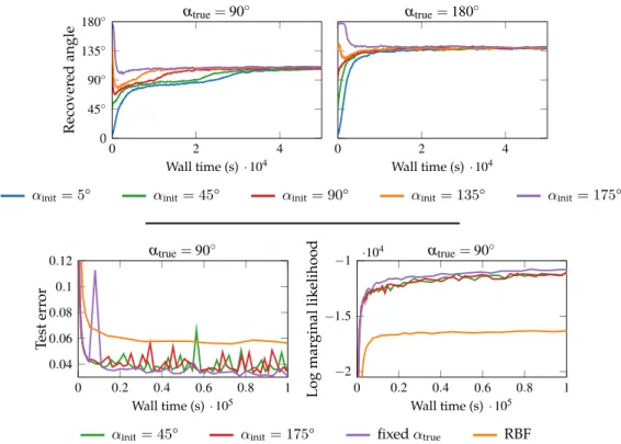
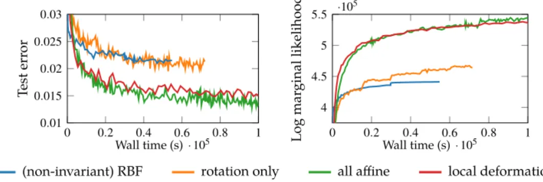
4.5 Empirical evaluation . . . 86
4.6 Discussion and outlook . . . 91
4.7 Summary . . . 93
II probabilistic inference in variational autoencoders 5 resampled priors for variational autoencoders 97 5.1 Problem statement . . . 98
5.2 Overview of the proposed solution . . . 100
5.3 Learned accept/reject sampling . . . 101
5.4 VAEs with resampled priors . . . 112
5.5 Experimental Setup . . . 115
5.6 Empirical evaluation: quantitative results . . . 116
5.7 Empirical evaluation: ablation studies . . . 118
5.8 Empirical evaluation: qualitative results . . . 120
5.9 Resampling discrete outputs of a VAE . . . 125
5.10 Comparison and relation to alternative approaches . . . 128
5.11 Summary . . . 130
III probabilistic inference in few-shot learning 6 introduction to few-shot learning 133 6.1 Transfer learning and meta-learning . . . 134
6.2 The few-shot learning task . . . 135
6.3 Our approaches to probabilistic few-shot learning . . . 137
6.4 Recent advanced in few-shot learning . . . 138
7 a probabilistic transfer approach to few-shot learning 143 7.1 A framework for probabilistic few-shot learning . . . 143
7.2 Choosing a model for the weights . . . 149
7.3 Empirical evaluation . . . 155
7.4 Summary . . . 165
8 meta-learning probabilistic inference for prediction 167 8.1 Meta-learning probabilistic inference for prediction . . . 168
8.2 Versatile amortised inference . . . 174
8.3 Ml-pip unifies disparate related approaches to few-shot learning . . . 178
8.4 Empirical evalution . . . 181
8.5 Discussion . . . 186
8.6 Summary . . . 189
Epilogue 9 discussion and conclusion 193 9.1 Overview of the main results . . . 193
9.2 Inductive biases in probabilistic modelling . . . 194
9.3 Model evaluation and benchmark datasets . . . 197
9.4 Advice for practitioners . . . 199
10 bibliography 203 Appendix a resampled priors for variational autoencoders 227 a.1 Experimental details . . . 227
b discriminative few-shot learning using probabilistic models 231 b.1 Experimental details . . . 231
c meta-learning probabilistic inference for prediction 233 c.1 Justification for the context-independent approximation . . . 233
c.2 Experimental details . . . 236
c.3 ShapeNet experimentation details . . . 238
Figure 1.1 Example regression problem for GP regression . . . 16
Figure 1.2 Posterior predictive distribution of exact GP inference . . . 17
Figure 1.3 Graphical model of a generic latent variable model . . . 22
Figure 2.1 Posterior predictive distribution for VFE using 15 inducing variables . 38 Figure 2.2 Factor graphs for the full GP and conditional independence approximation 39 Figure 2.3 Schematic illustration of the low rank approximation of the covariance matrix . . . 39
Figure 2.4 Graphical model for FITC and FIC . . . 42
Figure 3.1 Sketch of configurations preferred by the individual terms of the objective function . . . 52
Figure 3.2 Behaviour of FITC and VFE on subset of 100 data points of the Snelson dataset for 8 inducing inputs . . . 53
Figure 3.3 Change of the objective and the predictive distribution when adding additional inducing inputs . . . 55
Figure 3.4 Predictive distributions for FITC and VFE with 15 inducing inputs . . . 62
Figure 3.5 Clumping of inducing inputs for two dimensional input . . . 63
Figure 3.6 Results of optimising VFE and FITC after initialising the inducing inputs at the data points . . . 64
Figure 3.7 Optimisation behaviour of VFE and FITC for varying number of inducing inputs compared to the full GP . . . 65
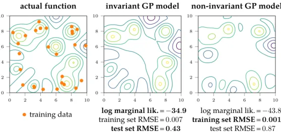
Figure 4.1 Data from a symmetric function with the solutions learned by invariant and non-invariant Gaussian processes . . . 75
Figure 4.2 Binary classification on the partially rotated MNIST dataset . . . 89
Figure 4.3 MNIST classification results . . . 90
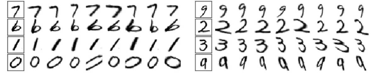
Figure 4.4 Samples describing thelearned invariancefor four example MNIST digits 91 Figure 4.5 Rotated MNIST classification results . . . 91
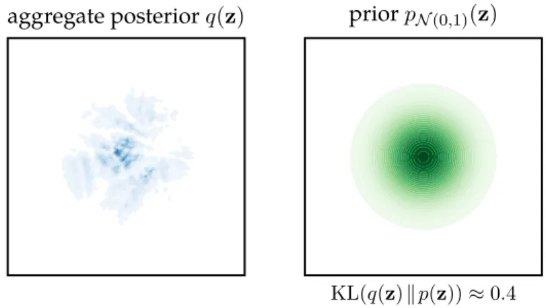
Figure 5.1 Illustrative example of the mismatch between aggregate posterior and prior . . . 99
Figure 5.2 Sample means from the matched region vs sample means from the mismatched region . . . 99
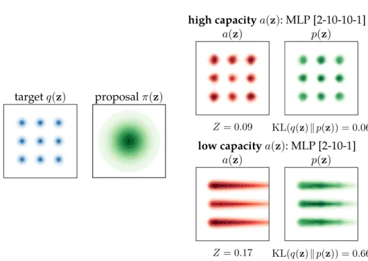
Figure 5.3 Lars approximates a target density by a resampled density . . . 101
Figure 5.4 Estimation ofZby MC sampling from the proposal . . . 107
Figure 5.5 Illustrative 2D example 1 . . . 110
Figure 5.6 Illustrative 2D example 2 . . . 111
Figure 5.7 Classic rejection sampling enables sampling from a complicated target distribution . . . 112
Figure 5.8 Hierarchical VAE with two latent spaces . . . 113
Figure 5.9 Ranked samples of a VAE with jointly trained resampled prior . . . 121
Figure 5.10 Ranked samples of a VAE with jointly trained resampled prior 2 . . . . 122
Figure 5.11 Ranked sample means from a VAE with post-hoc trained resampled prior123 Figure 5.17 Samples from a VAE with a jointly trained acceptance function on the output . . . 127
Figure 6.1 The few-shot learning task from a transfer-learning perspective . . . . 136
Figure 6.2 The few-shot learning task from a meta-learning perspective . . . 137
Figure 7.1 t-SNE embedding of the CIFAR-100 weights trained using a VGG style architecture . . . 144
Figure 7.2 Two-head model for probabilistic few-shot learning . . . 145
Figure 7.3 Graphical model for probabilistic few-shot learning. . . 146
Figure 7.4 Results on CIFAR-100 with VGG style architecture . . . 159
Figure 7.5 Comparison of different network architectures and training set sizes on the few-shot learning task . . . 162
Figure 7.6 Probabilistic few-shot learning results for the miniImageNet dataset utilising different network architectures and representational training . 163 Figure 7.7 Choice of regularisation constant for logistic regression for few-shot learning . . . 164
Figure 7.8 Online learning with ResNet-34 features . . . 166
Figure 8.1 Directed graphical model for multi-task learning . . . 169
Figure 8.2 Computational flow of Versa for few-shot classification with the context-independent approximation . . . 175
Figure 8.3 Computational flow of Versa for few-shot view reconstruction . . . 177
Figure 8.4 Comparison of true and amortised approximate posteriors (Versa) for unseen test sets . . . 182
Figure 8.5 Test accuracy on Omniglot when varying way and shot . . . 185
Figure 8.6 Results for ShapeNet view reconstruction for unseen objects from the test set . . . 187
Figure C.1 Visualising the learned weights fordϕ = 16 . . . 234
Figure C.2 Visualising the task weights fordϕ= 2 . . . 235
L I S T O F TA B L E S Table 3.1 Results for pumadyn32nm dataset . . . 66
Table 4.1 Final test error for MNIST classification results using a Gaussian likelihood. 90 Table 5.1 Test negative log likelihood for different models with standard Normal prior and our proposed resampled prior . . . 116
Table 5.2 ELBO and its components (KL and reconstruction error) for VAEs with standard and resampled prior . . . 116
Table 5.3 Test NLL on dynamic MNIST for non-convolutional and convolutional models . . . 117
Table 5.4 Test NLL on dynamic Omniglot. . . 117
Table 5.5 Test NLL andZ on dynamic MNIST. Different network architectures for a(z) . . . 118
Table 5.6 Influence of the truncation parameter on the test set of dynamic MNIST 119 Table 5.7 More expressive proposal and prior distributions on dynamic MNIST . 120 Table 5.8 More expressive proposal and prior distributions on dynamic Omniglot 120 Table 5.9 Test NLL on dynamic MNIST for a VAE withresampled outputs. . . 127
Table 7.2 Methods and inference procedure during phase 3 (few-shot learning) . 157
Table 7.3 Held-out log probabilities of the training weights for the different models on CIFAR-100 . . . 158
Table 7.4 Accuracy on 5-way classification onminiImageNet . . . 161
Table 8.1 Accuracies for different few-shot settings on Omniglot andminiImageNet184
Table 8.2 Negative log-likelihood (NLL) results for different few-shot settings on Omniglot andminiImageNet . . . 185
Table 8.3 View reconstruction test results . . . 186
Table B.1 Network architecture for a ResNet-34 inspired network for few-shot learning onminiImageNet . . . 231
Table B.2 Network architecture for a VGG inspired network for few-shot learning on CIFAR-100 andminiImageNet . . . 232
Table C.1 Feature extraction network used for Omniglot few-shot learning . . . . 237
Table C.2 Feature extraction network used forminiImageNet few-shot learning . 237
Table C.3 Amortisation network used for Omniglot andminiImageNet few-shot
learning . . . 238
Table C.4 Linear classifier used for Omniglot andminiImageNet few-shot learning 238
Table C.1 List of ShapeNet categories used in the Versa view reconstruction experiments. . . 239
Table C.2 Encoder network used for ShapeNet few-shot view reconstruction . . . 239
Table C.3 Amortisation network used for ShapeNet few-shot view reconstruction 239
Table C.4 Generator network used for ShapeNet few-shot learning. No dropout or batch normalisation are used. . . 240
L I S T O F A L G O R I T H M S
1 Estimation oflogZin the objective during training . . . 109 2 Pseudo code for training of a VAE with resampled prior . . . 114
0
I N T RO D U C T I O NP
robabilistic machine learning takes into account uncertainty on a funda-mental level; its probabilistic framework explains how to represent, reason about, and manipulate uncertainties. Probabilistic modelling has therefore become a cornerstone of “scientific data analysis, machine learning, robotics, cognitive science, and artificial intelligence” (Ghahramani,2015); fields in which the under-standing and consideration of uncertainties is paramount.In the probabilistic framework we describe our beliefs about the world and our models using probability theory. By writing down a probabilistic model, we express the connections between the known knowns, i.e. observations, and known unknowns, such as latent structures, latent variables, or random noise. Using Bayes’ rule we can infer likely values and even full distributions of unknown quantities from known quantities.
When facing a particular problem or task, the two main questions in probabilistic modelling and machine learning are (i) how to choose the probabilistic model describing the data, and (ii) how to perform probabilistic exact or approximate inference in this model. While model specification and inference are separate steps, they are often linked, as the complexity of the inference step depends on the model structure and distributions.
In general, we specify a probabilistic model by specifying a joint distribution of observations (known quantities) and latent variables (unknown quantities). Equivalently, we can define a prior distribution on the latent variables and a probability distribution that links them to the observations, which is termed the likelihood of the latent variables.
The choice of model, its structure, and particularly its prior heavily influence the encoded implicit or explicit inductive biases and, therefore, our ability to learn and generalise from data as well as the data efficiency associated with it. In principle, a large number of possible generalisations are consistent with a set of observations such that we need to make certain assumptions as specified through inductive biases to reduce them to a small and plausible set (Mitchell, 1980). Consider as an example the universal approximation theorems that famously state, that a single- or multi-layer feed-forward neural network of sufficient but finite size can approximate any continuous function with compact support (Cybenko, 1989; Hornik et al.,1989). However, for an arbitrary function it is unclear how to learn the corresponding weights, that is, which of the many model configurations to prefer. Yet by choosing a model with the right inductive biases for the problem
at hand, we can accurately learn relatively complex functions from small amounts of data. In other words, the model structure and its priors make it more prone to model certain functions than others. The choice and number of hidden layers and units, their weight sharing (such as convolutional layers), and non-linearities influence the typical functions represented by a neural network. Similarly the choice of covariance function affects all properties of typical sample draws from a Gaussian process, such as smoothness or stationarity.
In this thesis we present theoretical analyses as well as algorithmic and modelling advances in three areas of probabilistic machine learning. They are all connected by the underlying question of how structural choices and priors affect the inductive biases of models, and our ability to learn and make inferences from data for the tasks at hand.
These choices also determine the tractability of probabilistic inference and the approximations that are likely to be successful. As a secondary theme, we therefore discuss approximate probabilistic inference through variational methods and how it affects learning in these cases.
The three areas of probabilistic machine learning addressed in this thesis are (i) supervised learning with sparse Gaussian processes and how to incorporate general invariances into their prior covariance functions; (ii) unsupervised learning with variational autoencoders and the role of their prior; and (iii) probabilistic models for supervised few-shot learning tasks.
overview and main contributions
This section gives a brief overview of these three topics. Within each topic we highlight our main results and present how they relate to the two main themes of this thesis: inductive biases through structure and priors, and approximate variational inference.
These results have led to articles which I co-authored with my supervisors and other colleagues in the community, and have been published at international conferences and workshops. Below, I cite the main references for each chapter; my own contributions are highlighted at the beginning of the respective chapters in the main part of the thesis.
1. Sparse Gaussian processes and invariant covariance functions
Gaussian process (GP) models are an important class of Bayesian non-parametric models. Originally developed for supervised regression tasks, they directly model the underlying latent regression function. The properties of these functions such
introduction 3
as smoothness, stationarity, or scales of typical fluctuation are defined by the kernel or covariance function of the GP. Due to these strong inductive biases, learning with GPs can be very data efficient and provide principled uncertainties. While inference in GP regression with Gaussian likelihoods is tractable, it is intractable for general likelihoods such as the Bernoulli or Multinomial used in GP classification. Moreover, even fully tractable inference may be computationally infeasible as the necessary inversion of the covariance matrix scales cubically with the size of the data. Therefore, two important research questions are: (i) what are the right inductive biases/how to choose the covariance functions and its properties; and (ii) how to make probabilistic inference in GP models tractable and scalable to large datasets.
• In Chapter 3we disentangle the theoretical properties and optimisation behaviour of two widely used sparse Gaussian process approximations, which are both based on a low-rank approximation of the exact covariance matrix. Our results allow us to explain earlier empirical findings in more detail. Moreover, we conclude that one of the approaches, a variational free energy approximation to the full Gaussian process model, is more principled and extensible and should be used in practice. This is joint work with Mark van der Wilk and Carl E. Rasmussen and was originally published as ‘Understanding Probabilistic Sparse Gaussian Process Approximations’ (Bauer et al.,2016).
• In Chapter 4 we focus on the Gaussian process priors and discuss how general symmetries can be integrated into GP priors andcan be learned
using the marginal likelihood. To make learning tractable in this setting, we develop an approximate inference scheme that makes use of the variational approach discussed earlier alongside several other recent improvements to GP inference for regression and classification. Our main finding is that the marginal likelihood can indeed be used to identify and learn symmetries and invariances from data. These results are joint work with Mark van der Wilk, ST John, and James Hensman and were originally published as ‘Learning Invariances using the Marginal Likelihood’ (van der Wilk et al.,
2018).
2. Flexible priors for variational autoencoders
A prominent class of unsupervised learning models are variational autoencoders (VAEs). Despite their name and superficial similarities to classical autoencoders, they are actually deep generative latent variable models. While probabilistic inference through amortisation is scalable, we can still ask how to incorporate structure, what the right inductive biases are, and how they should affect the
design of the model. A VAE model is specified by fixing a prior distribution on latent codes as well as a likelihood of the latent codes for the corresponding observations.
• Prompted by recent research we discuss the role of the prior in variational autoencoders (VAEs) in Chapter 5 and propose a mechanism to define flexible distributions using a form of rejection sampling that we refer to as
learned accept/reject sampling(Lars). We then use this approach to define
a more flexible prior distribution on the latent space of a VAE, which generalises to unseen test data and reduces the number of low quality samples from the model. These findings are joint work with Andriy Mnih and were first published as ‘Resampled Priors for Variational Autoencoders’ (Bauer and Mnih,2019).
3. Probabilistic approaches to few-shot learning
In the last part of the thesis, we propose two probabilistic approaches to few-shot learning. The aim of a few-shot learning task is to classify instances based on very few examples per class with access to a large repository of related tasks on different classes. Because of the limited number of examples, uncertainty is rife, such that a probabilistic approach is appropriate. The two predominant perspectives on this task are: (i) transfer learning and (ii) meta-learning. Transfer learning addresses how previously acquired knowledge and representations can be leveraged to improve performance on a new but related task. Meta-learning instead emphasises meta-algorithms that can adapt a model or learner to new tasks, treating the training repository as a collection of many smaller tasks.
• InChapter 7 we follow the transfer learning perspective and show that a surprisingly simple probabilistic model for the head of a pretrained deep classifier often works well for this task and can outperform more complicated approaches. We can recast a special case of our model as automatically regularised softmax regression; the automatic regularisation also allows for efficient and balanced online learning when evaluating not only on new classes but also on the base classes. The probabilistic model for concept transfer is key and inductive biases in the model as well as the choice of the prior influence the final performance. This chapter is based on joint work with my co-first author Mateo Rojas-Carulla as well as Jakub Świ ˛atkowski, Bernhard Schölkopf, and Richard Turner and was published as ‘Discriminative k-shot learning using probabilistic models’ (Bauer*, Rojas-Carulla* et al.,2017b).
• While our previous approach requires a pretrained model as well as meta-test time optimisation, in Chapter 8 we present an extended model in
introduction 5
the vein of meta-learning. It is trained episodically and allows for fast meta-test time adaptation through amortised inference of the head model. Through episodic training and the model structure, weimplicitlylearn a
prior for the head weights, resulting in state-of-the-art performance on several benchmark datasets. These results are joint work with Johnathan Gordon, John Bronskill, Sebastian Nowozin, and Richard Turner and were published as ‘Meta-Learning Probabilistic Inference for Prediction’ (Gordon*, Bronskill* et al.,2019).
automatic estimation of modulation transfer functions
In addition to Bayesian probabilistic inference, I have also carried out research in the field of computational photography. This work is not covered in this thesis. Most notably, we have developed a method to estimate a physical quality metric of a camera and its lens, the so-calledmodulation transfer function, directly from a
set of photographs rather than measuring it in an optics laboratory. This work and related projects involved building custom hardware to collect a data set of ground truth lens properties, capturing a data set of photographs for training and evaluation, as well as designing and training the entire machine learning pipeline. These results are joint work with Michael Hirsch, Valentin Volchkov, and Bernhard Schölkopf and were published as ‘Automatic estimation of modulation transfer functions’ (Bauer et al.,2018).
list of publications
The following provides a list of all publications I have co-authored throughout my PhD, regardless of whether they appear in this thesis or not.
Conference proceedings:
Matthias Bauer, Mark van der Wilk, and Carl Edward Rasmussen (2016). ‘Understanding Probabilistic Sparse Gaussian Process Approximations’. In:
Advances in Neural Information Processing Systems 29
Matthias Bauer, Valentin Volchkov, Michael Hirsch, and Bernhard Schölkopf (2018). ‘Automatic estimation of modulation transfer functions’. In:2018 IEEE International Conference on Computational Photography (ICCP)
Mark van der Wilk, Matthias Bauer, ST John, and James Hensman (2018). ‘Learning Invariances using the Marginal Likelihood’. In:Advances in Neural
Jonathan Gordon*, John Bronskill*, Matthias Bauer, Sebastian Nowozin, and Richard Turner (2019). ‘Meta-Learning Probabilistic Inference for Prediction’. In:Proceedings of the 7th International Conference on Learning Representations.
*equal contribution
Matthias Bauer and Andriy Mnih (2019). ‘Resampled Priors for Variational Autoencoders’. In:Proceedings of the 22nd International Conference on Artificial Intelligence and Statistics
Frederik Harder, Matthias Bauer, and Mijung Park (2020). ‘Interpretable and Differentially Private Predictions’. In:Proceedings of the Thirty-Fourth AAAI Conference on Artificial Intelligence. New York, USA: AAAI Press
Journal articles:
Matthias Bauer*, Johannes Knebel*, Matthias Lechner, Peter Pickl, and Erwin Frey (2017a). ‘Ecological feedback in quorum-sensing microbial popula-tions can induce heterogeneous production of autoinducers’.eLife. *equal
contribution
Workshop contributions:
Matthias Bauer*, Mateo Rojas-Carulla*, Jakub B. Świ ˛atkowski, Bernhard Schölkopf, and Richard E. Turner (2017b). ‘Discriminative k-shot learning using probabilistic models’. In:Second Workshop on Bayesian Deep Learning at the 31st Conference on Neural Information Processing Systems. *equal contribution
Jonathan Gordon*, John Bronskill*, Matthias Bauer*, Sebastian Nowozin, and Richard E. Turner (2018b). ‘Versa: Versatile and Efficient Few-shot Learning’. In:Third Workshop on Bayesian Deep Learning at the 32nd Conference on Neural Information Processing Systems. *equal contribution
Jonathan Gordon*, John Bronskill*, Matthias Bauer*, Sebastian Nowozin, and Richard E. Turner (Dec. 2018a). ‘Consolidating the Meta-Learning Zoo: A Unifying Perspective as Posterior Predictive Inference’. In:Workshop on Meta-Learning (MetaLearn 2018) at the 32nd Conference on Neural Information Processing Systems. *equal contribution
1
BAC KG RO U N DI
n this chapter, we provide the necessary background for this thesis. We give a high-level introduction to probabilistic machine learning (Section 1.1) and highlight the role of the marginal likelihood for model selection and training (Section 1.2). We then discuss variational inference (Section 1.3) before introducing the two main model classes in this thesis, Gaussian processes (Section 1.4) and variational autoencoders (Section 1.6).1.1 probabilistic machine learning
This section introduces the basic concepts in probabilistic machine learning relevant to this thesis, with an emphasis on probabilistic modelling and inductive biases.
In the probabilistic framework we describe our beliefs about the world and our models using probability theory. By writing down a probabilistic model, we express the connections between the known knowns, i.e. observations, and known unknowns, such as latent structures, latent variables, or random noise.
We can then use the rules of inverse probability to infer likely values or whole distributions for unknown quantities from known quantities. Typically, the known quantities are observations at certain locations of the input space – here simply termed “data” – whereas unknown quantities can be model parameters, latent variables, the model structure, or predictions at yet unobserved locations of the input space – in the following also termed “hypothesis”. The main tool in this
context is Bayes’ rule, which can be derived from the sum and the product rule of Bayes’ rule probability and can abstractly be expressed as (e.g. MacKay (2003)):
p(hypothesis|data) = p(data|hypothesis)P × p(hypothesis) hp(data|h)p(h)
More formally, we can express Bayes’ rule in terms of observed dataDand model
parametersθfor a fixed modelm
p(θ| D, m) = p(D |θ, m) × p(θ|m)
p(D |m) (1.1)
posterior =
likelihood × prior
evidence .
The unknownposteriorappears on the left hand side ofEquation (1.1), whereas
all quantities that are known in principle appear on the right hand side of
Equation (1.1). Thepriorexpresses our belief about how likely certain hypothesis
are before having observed any data; the likelihood expresses how likely the
observed data are under a given hypothesis. Theevidenceacts as a normaliser for
the posterior, p(D |m) = Z p(D, θ|m) dθ= Z p(D |θ, m)p(θ|m) dθ, (1.2) and plays a crucial role in model selection and training of model parameters. It is also referred to as themarginal likelihoodand is the probability of the data
integrated over all hypotheses. We further discuss the marginal likelihood in
Section 1.2.
While all quantities within the evidencep(D |m)– the prior and the likelihood – are known, it is usually intractable to perform the sum or integral to marginalise over all the hypotheses or model parametersθ. We therefore have to resort to different approximation techniques in order to performapproximate inferencein
these intractable models, seeSection 1.3.
We can view Bayes’ rule as an update rule for the prior; our initial belief as expressed by the prior distribution is updated by observations through the likelihood. The posterior distribution then represents our updated belief about the world; it effectively acts as new prior that can be further updated by future observations. We can then use the posterior to make probabilistic predictions at new locationsD∗
p(D∗ | D, m) = Z
p(D∗|θ, m)p(θ| D, m) dθ (1.3)
In general, the posterior will not be of the same functional form as the prior, such that each Bayesian update gives rise to a more complex posterior distribution. A special case arises when the prior and likelihood areconjugate, that is, they are
conjugate models
such that the posterior is of the same functional form as the prior – in this case, Bayesian updates correspond to simple updates of the parameters of the prior
probabilistic machine learning 9
distribution. Conjugate distributions exist when the likelihood is a member of the exponential family (e. g. Murphy (2012)).
When faced with a particular task or problem, the two main steps in probabilistic modelling and machine learning are to (i) write down a probabilistic model that connects known and unknown quantities and (ii) perform exact or approximate inference in this model (Ghahramani,2013).
To write down a probabilistic modelm, we first choose the random variables of probabilistic model interest that denote known and unknown quantities, such as observables, latent
variables, or model parameters. To write down the “joint probability distribution of everything” (MacKay,2003) we then specify how these variables are connected
to each other. This model structure is often depicted through agraphical model graphical model that expresses conditional dependencies and independencies and details how
the joint distribution of all variables factorises. Finally, we need to specify the particular distributions of each factor, that is, the parametric or non-parametric form of the distributions as well as their parameterisation.
In an abstract example of a model with dataD and parametersθ, the joint probability distribution of the data and the model parameters, p(D, θ | m) factorises into a likelihoodp(D |θ, m)and a prior of the parameters p(θ |m). While the likelihood incorporates observations and is data-dependent, the prior should, in principle, only encode our prior beliefs and be data-independent. As a concrete example, consider a Bayesian neural network (BNN) (Neal,1994; MacKay, 1995) for regression, where the likelihood is Gaussian with mean expressed through a neural network with individual weightsθon which we place a prior.
Both of these design choices – the model structure and the individual dis-tributions, most notably the priors – fundamentally influence the properties and performance of our model and its ability to learn and generalise from data.
Crucially they encapsulate theinductive biases, by which we mean “biases for inductive biases choosing one generalization [sic] over another, other than strict consistency with
the observed training instances” (Mitchell,1980). In other words, in principle, a large number of possible generalisations are consistent with a set of observations such that we need to make further assumptions to reduce them to a small and plausible set. In the introduction we mentioned the universal approximation theorem that states that a single layer feed-forward network of sufficient size can realise any continuous function. In the above example of a BNN, the prior on the individual network weights induces a distribution of “typical” functions that the BNN can express. By altering the network architecture (layers, number of units, weight-sharing, non-linearities, etc.) or the prior on the weights, certain
functions become more or less likely. However, because we place a prior on the individual weights, it is hard to characterise this typical set. In contrast, the covariance function of a Gaussian process prior specifies global properties of typical function draws such as smoothness, periodicity or stationarity. This property makes Gaussian process models particularly amenable for Bayesian modelling, especially when we have expert knowledge about typical functions that we would like to encode. For example,Chapter 4describes the construction of a GP covariance function that respects general invariances – a property that would be hard to encode in neural networks. Interestingly, in the limit of infinite width a single layer BNN with independent Gaussian prior on the weights converges to a Gaussian process with a particular non-stationary covariance function (Neal, 1994; Williams,1998).
To reiterate, once the model structure or model class is fixed, the prior expresses prior
oura prioribelief about how likely each realisable model configuration is. While
the likelihood term can up- or down-weight the probability of each of these configurations, it cannot recover configurations that have zero probability under the prior. It is therefore important to make the prior sufficiently broad.
The prior itself may often contain hyperparametersλ, such as the parameters of the Gaussian process covariance function or the scale parameters of a Gaussian prior on the weights of a BNN. In a fully Bayesian treatment, we would also need to infer the values of these parameters through Bayesian inference, which requires ahyperprioronλ. This can lead to a cascade of higher and higher order priors
(Murphy,2012). The influence of these parameters often diminishes such that the model becomes increasingly insensitive to them, so this hierarchy is usually truncated at the first level. The hyperparametersλare then learned or optimised using the objective function directly; this approach is often referred to astype II maximum likelihood learning(Rasmussen and Williams,2006) orempirical Bayes. As
type II maximum
likelihood in conventional maximum likelihood learning, this can lead to overfitting. Many tasks within machine learning can be divided intosupervisedand unsuper-visedtasks. In supervised learning, we aim to predict some quantityy∈ Y given
supervised learning
an inputx∈ X from a limited number ofN training examplesD={xn, yn}Nn=1. The held-out data at which we evaluate our models performance is usually referred to as the test setD∗ ={x∗
n, y∗n}N ∗ n=1.
In unsupervised learning, the training and test sets only consists of unlabelled unsupervised
learning observations or targets,
D ={xn}N
n=1 andD∗ ={x∗n}N ∗
n=1 respectively, and the tasks are much more diverse. They range from clustering data into groups, learning representations, compressing data, uncovering hidden structure, or building a density model. In general, unsupervised learning models contain
probabilistic machine learning 11
latent structures and variables, such as cluster centroids and assignments, latent codes, or topic membership, that we wish to infer.
Supervised learning tasks can be further divided intoregressionandclassification
tasks. In regression tasks the outputsynare modeled as continuous functions regression of the inputs xnand can be single or multi dimensional. A typical likelihood
function in a probabilistic regression model is Gaussian observation noiseon top of a linear or non-linear transformation of the inputs,f(x),
y=f(x) + ∼ N(0, σ2). (1.4)
f(x)is also referred to as theregression function.
In contrast to regression, the outputs in classification tasks are typically discrete classification and are referred to aslabels; every input is categorised into one out ofCpossible
classes. Typical likelihoods for classification are the Bernoulli likelihood (for binary classification) or the Categorial likelihood (for more than two classes). These likelihoods can be expressed through the softmax function
p(y=c|x, θ) = e Φϕ(x)Twc P c0eΦϕ(x) Tw c0 , (1.5)
whereΦϕ(x)is a linear or non-linear transformation (with parametersϕ) of the
inputs including a constant output to model biases,wcdenotes the weights for
classc, andθdenotes the collection of all parameters.Φϕ(x)is also referred to as feature representationof the inputx.
In the case of binary classification, the softmax function inEquation (1.5)can be simplified to a sigmoid functionσand the likelihood is given by
p(y=c1 |x, θ) =σ(Φϕ(x)Tw1) (1.6)
p(y=c2 |x, θ) = 1−σ(Φϕ(x)Tw1) (1.7)
Orthogonal to the division into supervised and unsupervised learning tasks, machine learning models can be divided into parametric and non-parametric
models.
The hallmark of parametric methods is that the involved regression functions, parametric methods feature representations, or distributions are explicitly parameterised in terms
of functions with a fixed, finite number of parameters. Examples of parametric methods range from simple linear or logistic regression to highly complex deep neural networks. While the capacity and expressiveness of these methods are very different, a common factor is that the capacity stays the same regardless of the size of the training data. This has the advantage of fixed computational cost but the disadvantage of not being able to extend capacity when data at new input locations is observed.
In contrast, the capacity of (Bayesian) non-parametric models grows with the Bayesian
non-parametrics training data size. However, this can lead to potentially prohibitive computational costs for large data. Parts of this thesis are concerned with Gaussian processes, a prominent class of Bayesian non-parametrics, which we introduce inSection 1.4. For an excellent recent survey on Bayesian non-parametrics refer to Ghahramani (2013).
1.2 the marginal likelihood
The evidence or marginal likelihood plays a crucial role in model selection and training of probabilistic models. This section elaborates on both these aspects and explains the built-in inductive biases for model selection: a Bayesian version of Occam’s razor. We use the marginal likelihood as a starting point to choose and optimise our models throughout this thesis.
Most current non-probabilistic machine learning models are trained by maxim-ising the likelihoodp(D |θ, m)with respect to model parametersθdirectly. One maximum likelihood
learning issue with this objective function is that it does not distinguish between models which fit the training data equally well but will have different generalisation characteristics. In an extreme case, some models may fit the training data better but generalise worse or not at all; when this happens, this is typically known as
overfitting. Some form of regularisation is often employed to avoid said overfitting,
overfitting
improve generalisation, or encourage other model properties such as sparsity. Nonetheless, it is usually difficult to assess these from the likelihood alone and validation sets or cross-validation techniques must be employed (Bishop,2006). The archetypal example of such a case is one of polynomial regression (see, for example, Rasmussen and Ghahramani (2001), Bishop (2006) and MacKay (2003)). In polynomial regression, models differ by the order of polynomials used as regression function to explain the data. In all cases, the learnable parametersθare given by the various coefficients. Typically, three (or more) cases are considered: (i) a very low order polynomialm1that is not flexible enough to fit the training data well; (ii) an intermediate order polynomialm2 that is just flexible enough; (iii) and a very high order polynomialm3that perfectly fits the training data for a very fine-tuned set of coefficients that typically lead to a strongly oscillating function.
When only considering the (training) likelihood,m3 will perform best andm1 will perform worst; however, we expectm2to generalise the best, followed by
m1and thenm3. The problem is that the likelihood does not take into account thecomplexityof the regression functions. Intuitively, we expect the model that
variational inference 13
overfit and model random noise. This heuristic is referred to asOccam’s razorand Occam’s razor is discussed in the context of machine learning by Jefferys and Berger (1992) and
Rasmussen and Ghahramani (2001). More generally Occam’s razor states that out of competing methods with same training set fit, one should prefer the one with fewest assumptions. By integrating the likelihood against the prior, the marginal likelihood takes complexity into account and penalises more complex models over simpler ones (Rasmussen and Ghahramani,2001; MacKay,2003; Rasmussen and Williams,2006). The marginal likelihood is also closely related to bounds on the generalisation error (Seeger,2003; Germain et al.,2016).
Intuitively, this complexity penalty is a volume argument: complex models (e.g. higher order polynomials) spread their prior mass over a larger space than simpler models (e.g. lower order polynomials); and while a particular fine-tuned configuration of a complex model may fit the training data extremely well, this configuration occupies a very small volume compared to the likely configurations of a simpler model. At the same time, an overly simplistic model might not be able to fit the data well at all. Choosing the right model is a matter of evaluating this trade-off. Rasmussen and Ghahramani (2001) make this argument more precise for several simple regression examples. They evaluate the marginal likelihood for different models of varying complexities and confirm that it rewards models with just enough but not too much complexity. Gaussian process models for regression and classification also allow for the marginal likelihood or good approximations of it to be evaluated (seeChapters 2and3) and are therefore accessible to a similar analysis. InSection 3.1we revisit the volume argument for the objective function of sparse Gaussian processes. InChapter 4we use Bayesian model selection and the log marginal likelihood to identify and learn invariances.
In summary, the marginal likelihood can be used to compare different models by applying Bayes’ rule at the level of the models instead of the parameters (e.g.
Ghahramani (2015) and MacKay (2003)): Bayesian model
selection
p(m| D) = p(D |m)p(m)
p(D) ∝p(D |m)p(m). (1.8)
1.3 variational inference
Exact inference is only possible in the simplest probabilistic models. As we alluded to above, in most cases the marginal likelihood is intractable, and solving the inference problem corresponds to computing the intractable high-dimensional evidence integral (Equation (1.2)). Fortunately, many approximation techniques
have been developed that allow us to performapproximate inferencein a growing approximate inference class of models. Most approaches fall in one of the following categories: Markov
(VI) (Jordan et al.,1999; Wainwright and Jordan,2007), expectation propagation (EP) (Minka,2001), or sequential Monte Carlo (SMC) (Doucet et al.,2000).
In this thesis, we focus on variational methods and therefore only introduce variational inference in detail. For the other approximation techniques, we refer the reader to the references above. Moreover, we focus on aspects of variational inference that are directly relevant to this thesis and refer the reader to Jordan et al. (1999) and Wainwright and Jordan (2007) for a detailed exposition, MacKay (2003) for a light introduction from a physics point of view, and Blei et al. (2017) for an excellent recent review.
Variational inference transforms an intractable integration problem into an Variational inference
optimisation problem. To do this, the intractable distributionp(z) is replaced by a flexible but usually simpler distributionqϕ(z), for which the integration
problem can be solved efficiently. We then aim to makeqϕas close topas possible
by adapting itsvariational parametersϕ. Formally, this is done by minimising the KL-divergenceor relative entropy fromqϕtop:
KL-divergence KL(qϕ(z)kp(z)) = Z qϕ(z) log qϕ(z) p(z) dz≥0 (1.9)
The KL divergence is asymmetric, always non-negative, and zero if and only ifqϕ
andpare equal. Its second order Taylor approximation is symmetric by design and the corresponding Hessian matrix is referred to as theFisher information matrix, which plays a crucial role in the field of information geometry (Amari, 2016). It can be used to define a distance metric between distributions as well as natural gradients, which can lead to drastically faster convergence rates for
gradient descent based algorithms; refer to Martens (2014) for a recent review. In practice, the approximating family of distributions{qϕ}ϕ often does not
contain the intractable distributionp(z), such that all solutions obtained even with the optimalq∗ϕare suboptimal compared to the true distributionp(z). The resulting difference to the true solution is referred to as theapproximation gap
approximation gap
(Cremer et al.,2018).
A common simple choice forqϕis the Normal distribution which often allows
us to compute integrals and moments in closed form. The variational parameters then correspond to its mean µ and covariance matrix Σ. In many cases the covariance is constrained to be diagonal or even isotropic to reduce the number of learnable parameters.
Variational inference can be applied both to global variables that affect all datapoints, such as the weight posteriors of a BNN (Blundell et al.,2015) or the inducing inputs of sparse Gaussian process approximations (Titsias,2009a), as
gaussian process methods 15
well as local per-datapoint variables, such as the approximate posterior in a latent variable model (seeSection 1.5). In the latter case, the model contains one or more variational parametersper datapointthat must be optimised.
This has several, usually negative, consequences which preclude scaling to larger datasets. The two main computational ramifications are: (i) the number of (local) variational parameters grows as the size of data set grows; (ii) after training the model, the (local) variational parameters for new test points still need to be optimised during test time. A solution to both these problems is
amortisedvariational inference; instead of optimising the per-datapoint variational amortised inference parameters directly, we train a so-calledinference,recognition, orencodernetwork
that outputs the variational parameters. The inference network has a fixed size and allows for fast test-time inference through a single forward pass. However, the resulting variational parameters may not be optimal for that particular datapoint.
This suboptimality is usually referred to asamortisation gap(Cremer et al.,2018). amortisation gap InSection 1.6we introduce a family of deep generative models called variational
autoencoders (P. and Welling, 2014; Rezende et al., 2014), which popularised amortised variational inference.
1.4 gaussian process methods
The first part of this thesis,Chapters 3and4, presents analyses and advances in Gaussian process models. In the following, we therefore provide an exposition of Gaussian processes for supervised learning with a focus on regression. We touch on classification and unsupervised learning with Gaussian processes in
Sections 1.4.3and1.5, respectively. For a comprehensive textbook on Gaussian processes in machine learning refer to Rasmussen and Williams (2006)
1.4.1 Inference in Gaussian processes for regression
Given a training dataset D of N observations of input/output pairs, D =
{(xn, yn) | n = 1, . . . , N}, we wish to make predictions y∗ at previously
un-observed test inputsx∗. We collect the training inputsxninto a matrixX and
the (possibly noisy) training outputs yn into a vector y. Typically, x is
multi-dimensional and continuous, whereasyis one-(or low-) dimensional and can be either continuous (in case of regression) or discrete (in case of classification). In the following, we use a one-dimensional dataset as an illustrative example, see
Figure 1.1.
In GP regression we model the outputsyby an (unobserved)latent functionf,
−1 0 1 2 3 4 5 6 7 −2 −1 0 1 2 inputsx outputs y [ 26th August 2019 at 11:34 – version 0.1 ]
Figure 1.1:Example regression problem from Snelson and Ghahramani (2006) for GP re-gression with one-dimensional inputsxnand noisy one-dimensional outputs yn.
Equation (1.4). With these assumptions, exact posterior inference is fully tractable as we discuss in the following.
Formally, “a Gaussian process is a collection of random variables, any finite number of which have a consistent1joint Gaussian distribution” (Rasmussen and Williams,2006, Definition 2.1). It is fully determined by its mean functionm(x)and covariance functionk(x,x0). The covariance function encodes our assumptions and inductive biases on the latent functionf, such as smoothness, amplitude, periodicity, or other symmetries. Intuitively, it defines a notion of similarity of inputs. When the covariance between two inputs is large, the corresponding function values co-vary. When it is small, the function values vary independently. For now, we assume the covariance function is given and discuss its choice in more detail inSection 1.4.2.
As stated above, we model the entire latent function f by a GP prior. By definition, a finite collection of latent function values at training inputsXand future test inputsX∗is assumed to have a joint Gaussian distribution:
f(·)∼ GP(0, k(·,·)) y p(f,f∗) =N 0, " Kff Kf∗ K∗f K∗∗ #! (1.10) wheref and f∗ denote the latent function values at the training inputsXand test inputsX∗, respectively, and we have introduced the covariance matrices [Kff]ij =k(xi,xj),[K∗f]ij =k(x∗i,xj), and so on. For simplicity we have assumed
the data to be zero-centred and stationary such that a zero mean function is appropriate. The training observationsyat the input locations are assumed to be
1 By “consistent” we mean that “the random variables obey the usual rules of marginalisation, etc.” (Quiñonero-Candela and Rasmussen,2005).
gaussian process methods 17
noisy observations around the latent function valuesf and are incorporated via the Gaussian likelihoodp(y|f):
p(y|f) = N Y n=1 N yn;fn, σn2 (1.11) where the scalarσ2nis referred to asnoise variance. In the noise free limit,σ2
n→0, noise variance the likelihood collapses to a delta-function aty=f. Other noise models are, of
course, possible; however, to obtain analytically tractable expressions a conjugate Gaussian likelihood is often used.
We obtain the joint posterior over the latent function values from Bayes’ rule: p(f,f∗ |y) = p(y|f)p(f,f∗)
p(y) (1.12)
As the prior and the likelihood are Gaussian, exact Bayesian inference is possible and the posterior predictive probability off∗is again given by a GP. It is obtained by marginalising over the latent function valuesf:
p(f∗ |y, X, X∗) = Z
p(f,f∗ |y, X, X∗) df =N(f∗ |µ∗,Σ∗) (1.13a)
µ∗ =K∗f[Kff +σn2I]−1y (1.13b)
Σ∗ =K∗∗−K∗f[Kff+σ2nI]−1Kf∗ (1.13c) Observe that the predictive mean is linear both in the observationsyand in the covariances with the test inputs,K∗f. The predictive covariance at the test points,
Σ∗is the original full covarianceK∗∗minus the conditional covariance that can already be explained by the training dataD.Figure 1.2illustrates the posterior
predictive distribution of exact GP inference for our illustrative example.
−1 0 1 2 3 4 5 6 7 −2 −1 0 1 2 inputsx outputs y [ 14th August 2019 at 15:46 – version 0.1 ]
Figure 1.2:Posterior predictive distribution of exact GP inference with a squared expo-nential kernel and learned hyperparameters. We plot the predictive mean (grey line) and two standard deviations (shaded area).
The log of the marginal likelihood is analytically tractable and obtained by marginalising over the latent regression functionf:
logp(y|X) = log Z p(y|f)p(f,f∗) dfdf∗ (1.14) =−1 2y T (Kff+σn2I)−1y− 1 2log Kff+σn2 −N 2 log 2π. (1.15) As discussed inSection 1.2we can use the marginal likelihood for model compar-ison to, for example, select suitable priors or tune the noise varianceσn2.
1.4.2 Covariance functions and hyperparameter learning
So far, we have assumed the covariance functionk(x,x0)to be given. But how should we choose it in practice? This usually depends on the task at hand; there exists an abundance of literature about this topic, for example, Rasmussen and Williams (2006, Chapter 4) and Duvenaud (2014).
The covariance function plays the same role as thekernelin Support Vector
Ma-kernel
chines (SVM); refer to Schölkopf and Smola (2002) and Steinwart and Christmann (2008) for two comprehensive books on SVMs and Stulp and Sigaud (2015) for an excellent review relating GPs to SVMs and other widely used (kernalised and non-kernalised) regression algorithms. Due to this close connection we use the terms covariance function and kernel function, or kernel for short, interchangeably.
As mentioned above, choosing a particular covariance function determines the properties of the latent functions that can be represented by the GP prior. Observations then restrict these functions further through their likelihood to, for example, pass through or close to certain points or have a certain derivative at a particular location.
A very popular choice for the covariance function in GPs is the squared exponential kernel
squared exponential
kernel
k(x,x0) =s2fexp(−12|x−x0|2/`2) (1.16) where the signal variances2f and the lengthscale`are thekernel hyperparameters.
kernel and model
hyperparameters Together with the noise varianceσ2
nof the likelihood they form the vectorθof model hyperparameters. The signal variance determines the scale on which the
latent function f varies, whereas the lengthscales determines how quickly it changes.
To make the functions invariant to finite shifts, that is, translations by a period T, we can include trigonometric functions, such as cosines, in the covariance function (MacKay,1998); inputs a period apart are then maximally correlated.
gaussian process methods 19
In Chapter 4 we construct a covariance function that can encode arbitrary general symmetries or invariances and can be used to learn them using the marginal likelihood.
In general, new kernels can be constructed out of existing kernels (Rasmussen and Williams,2006, Section 4.2.4): Ifk1andk2are valid covariance functions on a domainX, so arek1+k2as well ask1×k2. Moreover, ifΦis a mapping between two sets,Φ :Xe_X, andkis a valid kernel onX thenk(Φ(x),Φ(x0))is a valid kernel on Xe. For example, by combining a squared exponential kernel and a periodic kernel, we can build a prior for functions with modulated periodicity.
Choosing the “right” covariance function is a highly non-trivial task. Fortunately, the marginal likelihood can be used to select the best model or covariance function out of several candidates. However, even enumerating the covariance functions that can be constructed by combining simpler kernels is already a combinatorial problem. Thus, a naive approach is infeasible. Several recent approaches attempt to automatically inferonegood covariance function from the data, such as the
automatic statistican (Steinruecken et al. (2019) provide a recent summary) or kernel discovery through latent space optimisation (Lu et al.,2018). In both of these cases, richer kernels are constructed out of simpler ones. Orthogonal to this, approaches such as deep kernel learning (DKL) (Wilson et al.,2016b) use deep neural networks to extract features from the inputs and apply a simple kernel to them.
Selecting the functional form of the kernel is only the first part of specifying the covariance function. We must also identify the best model hyperparameters. As discussed inSection 1.1there are two basic ways to set the hyperparameters of a probabilistic model: (i) a fully Bayesian treatment: place a hyperprior on the hyperparameters and then perform Bayesian inference on them as well; (ii) type II maximum likelihood learning: directly optimise the marginal likelihood w.r.t.θ. While (i) is more principled, it is also often infeasible. In practice, one
frequently resorts to (ii) and chooses the hyperparameters that optimise the log marginal likelihood. However, this is usually a non-convex optimisation problem with local minima and saddle points. Moreover, it may lead to overfitting (refer to the discussion in Section 1.4.4 and Chapter 3) or, indeed, underfitting; for example, when GPs are fit to a very small number of points in this way they often over-estimate the lengthscale.
Both approaches for choosing hyperparameters in a principled way constitute one major advantage of GPs over other kernel methods; for the latter, there is no such clear cut objective which often necessitates cross-validation or learning the kernel matrix (Bousquet and Herrmann,2003).
1.4.3 Gaussian process models for classification
So far we have explained Gaussian process regression with a Gaussian likelihood function. In classification, the outputsyare no longer continuous but discrete – every inputxbelongs to one out ofCpossible classes. Here, we briefly discuss Gaussian process classification. Fore a more in-depth introduction see Rasmussen and Williams (2006, Chapter 3).
A first approach is to ignore the discreteness of the classes and model the label with a Gaussian likelihood regardless. We take this approach in parts of
Chapter 4as our estimators of the objective there are only unbiased for Gaussian likelihoods. Using a Gaussian likelihood has the advantage that we can use the machinery developed for regression; however, it has several disadvantages. Foremost, our modelling assumptions are clearly violated, which can lead to poor predictive performance. Second, our predictive uncertainty becomes meaningless. Moreover, especially when modelling more than two classes with this approach, we implicitly assume an ordering of the classes that is not founded in reality – 1 would be closer to 2 than to 4, for example. Though, modelling several one-hot encoded outputs with Gaussian likelihoods instead can alleviate this problem and often works well in practice.
The more principled approach uses classification likelihoods (Rasmussen and Williams,2006). In the case of binary classification, we place a GP prior on the latent functionf(x), which is subsequently squashed by a logistic function to model the prior distribution
π(x) =p(y= 1|f(x)) =σ(f(x)). (1.17)
Similarly to the regression case, inference consists of computing the posterior distribution of the latent functionf∗at a new inputx∗and integrating it over the likelihood: p(f∗|X,y,x∗) = Z p(f∗ |X,x∗,f)p(f |X,y) df (1.18) p(y∗= 1|X,y,x∗) = Z σ(f∗)p(f∗ |X,y,x∗) df∗. (1.19) Because of the non-conjugate likelihood, inference is analytically intractable and we must apply approximations. InSection 2.5we describe a variational approach for large scale classification.
continuous latent variable models 21
1.4.4 Notes on implementations and libraries
To compute the marginal likelihood inEquation (1.14)and make predictions, we must compute the inverse and log-determinant of the kernel matrixKff+σn2I.
For numerical stability these computations are performed using the Cholesky decomposition,Kff+σn2I =LLT, whereLis a lower triangular matrix. Moreover,
kernel matrices without noise, such asKff by itself, can become singular, such
that their inverse might not exist. In such cases, a small diagonal jitter-term
is added to ensure non-singularity. We will discuss the influence of this term further inChapter 3.
The optimisation of the marginal likelihood w.r.t. the hyperparameters is often performed using second order gradient methods such as L-BFGS (Liu and Nocedal,1989). For these, the gradients of the objective w.r.t. the hyperparameters are needed. For their computation and, in fact, many of the computations associated with GPs,The Matrix Cookbook(Petersen and Pedersen, 2012) is an
invaluable resource. For further details on the implementation of GPs, refer to the documentation of standard toolboxes such asgpmlformatlab(Rasmussen and
Nickisch,2010),GPyforpython(The GPy authors,2012), orGPflow(Matthews
et al.,2017) forpythonusingtensorflow(Martín Abadi et al.,2015).
All exact implementations of fully general GPs scale asO(N3) in time and
O(N2)in memory complexity, whereN is the number of training inputs. This is due to the computation of the log-determinant and the inverse of the covariance matrix; computing the eigenvalues and the Cholesky decomposition takesO(N3). This limits exact GP inference to small to medium sized datasets with on the order of 10,000 data points in many ways.
A growing number of approximate inference techniques allow us to scale Gaussian process inference beyond these limitations. InChapter 2we introduce several of these approximation techniques and analyse two of them in depth in
Chapter 3.
1.5 continuous latent variable models
So far we have described supervised learning methods, which map inputsxto outputsy. A second pillar of machine learning isunsupervised learning, in which
we aim to model inputsxor their densitypData(x), usually by means of some form of latent structure or variables. Often these help us to interpret the data without labels and uncover its structure.
In the second part of this thesis we discuss the priors in variational autoencoders (VAEs), which are an example of continuous latent variable models with a
particular inference scheme. This section introduces continuous latent variable models in general before we discuss VAEs in more detail inSection 1.6.
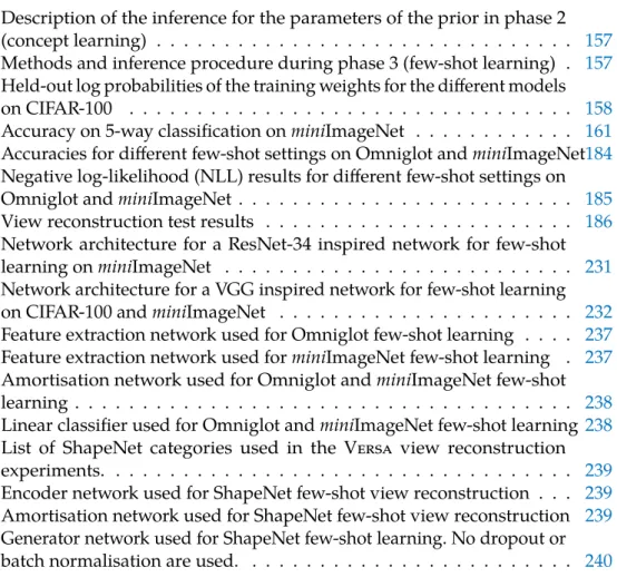
Continuous latent variable models (LVMs) are one type of unsupervised probabilistic model that explain observablesxthrough unobserved continuous latent variablesz. More specifically, we use continuous latent variable models to model a high-dimensional data distributionpData(x) by means of a simple prior distributionpλ(z)in a latent space, which is warped by a likelihood model
pθ(x|z)to fit the data, seeFigure 1.3.
z
p
λ(
z
)
x
p
θ(
x
|
z
)
q
ϕ(
z
|
x
)
Figure 1.3:Graphical model of a generic latent variable model with prior pλ(z) and
likelihood pθ(x|z). To perform (amortised) variational inference, we also
include a parametrised inference distribution qϕ(z|x) also referred to as
approximate posterior.
Formally, a LVM is defined through a joint probability of observed and un-observed variables pθ(x,z). Using the product rule of probability, this joint
probability is factorised into a priorpλ(z)and a likelihoodpθ(x|z),
pθ,λ(x,z) =pλ(z)pθ(x|z), (1.20)
whereλandθdenote the free parameters of the prior and likelihood, respectively. Thus, we can define a latent variable model by specifying the prior on the latent codes and the data likelihood under those codes. The latent variableszcan be both discrete and continuous; here, we focus on the latter. Usually, we choose the prior to be a standard Normal distribution,p(z) =N(0,1).
The model distribution is then given by the marginal likelihood pθ(x) =
Z
p(z)pθ(x|z) dz, (1.21)
1.5.1 Examples of continuous latent variable models
continuous latent variable models 23
linear gaussian model
A Gaussian likelihood model with linear mean function and isotropic covariance corresponds to probabilistic principal component analysis (PCA) (Tipping and Bishop,1999; Roweis,1998):
x=Wz+ ∼ N(0, σ21) (1.22)
In this case, the model allows for an exact closed-form solution, which is defined up to arbitrary orthogonal rotations of the latent space (Tipping and Bishop,1999). Probabilistic PCA is closely related to factor analysis (Spearman,1904), which assumes diagonal but not necessarily isotropic covariance; factor analysis no longer allows for a closed-form solution of the weightsW but iterative methods exist (Rubin and Thayer,1982). non-linear gaussian process model
A simple yet flexible non-linear model is the Gaussian Process Latent Variable Model (GP-LVM) (Lawrence,2004), which uses a GP to model the mean of a Gaussian likelihood with isotropic covariance:
x=f(z) + f ∼ GP(µ, K); ∼ N(0, σ21) (1.23) As the prior distribution on the latent space is warped through a non-linear function, exact inference is impossible. Titsias and Lawrence (2010) proposed a variational approach to obtain a lower bound to the marginal likelihood, following earlier works on variational inference for GP regression (Titsias, 2009a).
non-linear neural network model
Instead of GPs we can also parametrise the likelihood function through a neural network. Besides Gaussian noise models, a range of likelihood distributions is used in practice, such as the Bernoulli distribution but also more complicated auto-regressive structures or the discretised mixture of logistics likelihood (Salimans et al.,2017). For these more complicated likelihoods we not only parameterise the means but also the other parameters of the likelihood, such as the scales or mixture components.
When this model is trained using amortised variational inference for the
approximate posterior, it is usually referred to as variational autoencoder (VAE) (P. and Welling,2014; Rezende et al.,2014), though strictly speaking it is not an autoencoder but a deep probabilistic latent variable model. We provide a more detailed introduction to VAEs inSection 1.6and discuss their priors inChapter 5.