Special Section on 3D Object Retrieval
Matching 3D face scans using interest points and local
histogram descriptors
$
Stefano Berretti
a,n, Naoufel Werghi
b, Alberto del Bimbo
a, Pietro Pala
a aDepartment of Information Engineering, University of Firenze, Italy
bKhalifa University of Science Technology & Research, Abu Dhabi, United Arab Emirates
a r t i c l e i n f o
Article history:Received 30 October 2012 Received in revised form 29 March 2013 Accepted 1 April 2013 Available online 1 May 2013
Keywords:
3D face recognition 3D keypoints 3D local descriptors
a b s t r a c t
In this work, we propose and experiment an original solution to 3D face recognition that supports face matching also in the case of probe scans with missing parts. In the proposed approach, distinguishing traits of the face are captured byfirst extracting 3D keypoints of the scan and then measuring how the face surface changes in the keypoints neighborhood using local shape descriptors. In particular: 3D keypoints detection relies on the adaptation to the case of 3D faces of the meshDOG algorithm that has been demonstrated to be effective for 3D keypoints extraction from generic objects; as 3D local descriptors we used the HOG descriptor and also proposed two alternative solutions that develop, respectively, on the
histogram of orientationsand thegeometric histogramdescriptors. Face similarity is evaluated by comparing local shape descriptors across inlier pairs of matching keypoints between probe and gallery scans. The face recognition accuracy of the approach has beenfirst experimented on the difficult probes included in the new 2D/3D Florence face dataset that has been recently collected and released at the University of Firenze, and on the Binghamton University 3D facial expression dataset. Then, a comprehensive comparative evaluation has been performed on the Bosphorus, Gavab and UND/FRGC v2.0 databases, where competitive results with respect to existing solutions for 3D face biometrics have been obtained.
&2013 The Authors. Published by Elsevier Ltd.
1. Introduction
The humans'cognitive system has a peculiar attitude in recogniz-ing faces with high accuracy, at least for familiar people in favorable viewing conditions (i.e., good illumination, small occlusions, etc.). Automatic identity recognition performed by machines has entered the scene some decades ago with the aim to extend the human capabilities by covering different and more general contexts. In particular, face has affirmed itself as one of the most important biometric trait due to the fact that images or videos of the face are collectable in an easy and non-intrusive way, whereas other bio-metrics, such asfingerprints or iris scans are impractical to implement in many scenarios (e.g., in a surveillance setting). Impressively, recent studies report that automatic face recognition can even outperform the human performance in some particular conditions[1]. However, the accuracy of automatic identity recognition based on faces still suffers from many factors, such as pose changes, illumination varia-tions, facial expressions and occlusions.
To solve these problems, face recognition using 3D scans of the face has been recently proposed as an alternative or complementary
solution to conventional 2D face recognition approaches using still images or videos, so as to allow accurate face recognition also in real-world applications with unconstrained acquisition. Confirming this recent research trend, several 3D face recognition approaches have been proposed and experimented in the last few years (see the survey in [2], and the literature review in [3–5] for a thorough discussion). However, many of the works appeared in this field, proposed conventional face recognition experiments, where both the probe and gallery scans are assumed to be acquired cooperatively in a controlled environment in which the whole face is precisely captured and represented. These methods mainly focussed on face recognition in the presence of expression variations, reporting very high accuracy on benchmark databases like the Face Recognition Grand Challenge (FRGC version 2.0)[6]. Recent studies also exploit ethnicity, gender and age to improve the accuracy of 3D face recognition[7,8]. Solutions enabling face recognition in uncoopera-tive scenarios are now attracting an increasing interest. In such a case, probe scans are acquired in unconstrained conditions that may lead tomissing parts(non-frontal pose of the face) or toocclusions due to hair, glasses, scarves, hand gestures, etc. These difficulties are further sharpened by the recent advent of 4D scanners (3D plus time)[9–11], capable of acquiring temporal sequences of 3D scans. In fact, the dynamics of facial movements captured by these devices can be useful for many applications [12,13], but also increases the acquisition noise and the variability in subjects' pose. In summary, techniques supporting 3D partial face matching are gaining Contents lists available atSciVerse ScienceDirect
journal homepage:www.elsevier.com/locate/cag
Computers & Graphics
0097-8493&2013 The Authors. Published by Elsevier Ltd. http://dx.doi.org/10.1016/j.cag.2013.04.001
☆To comment on this article, please join the discussion on the Collage Authoring Environment Google Group https://groups.google.com/group/collage-authoring-environment.
n
Corresponding author. Tel.:+39 55 4796415; fax:+39 55 4796493.
E-mail addresses:[email protected]fi.it, stefano.berretti@unifi.it (S. Berretti).
Open access under CC BY-NC-ND license.
importance in making 3D face recognition techniques deployable in more general contexts and, in perspective, in scenarios where 3D dynamic acquisition is performed. However, the research in this context is still preliminary also due to the limited number of face databases that also comprise partial acquisitions of 3D faces
[14–16].
1.1. Related work
Below, we review the most recent methods for 3D face recogni-tion, by limiting our analysis to the works that also propose and evaluate solutions supporting partial match of 3D facial scans. In particular, we focus on methods that were also evaluated on scans acquired from non-frontal views of the face for which the recognition problem is further complicated by artifacts that alter the geometry of the acquired 3D surface in correspondence to the borders of the missing regions, rather than to solutions that just cropped 3D full face scans to simulate missing parts. In general, existing solutions can be grouped asglobalandlocal;Multimodalapproaches that combine together 2D and 3D methods are also possible.
Global 3D face representations for partial face matching have been proposed in a limited number of works. The first solutions appeared in this category used the Iterative Closest Point (ICP) algorithm[17]. The method proposed in[18], was global and multi-modal trying to combine 3D shape and 2D texture to perform surface and appearance-based matching. The surface matching component was based on a coarse tofine alignment between a 2.5D probe and a fully 3D face model (obtained by the fusion offive 2.5D scans). In the coarse step,first three manually labeled generic points were used to calculate the rigid transformation that aligns the 2.5D scan with the 3D model, then specific feature points are identified by finding correspondence between shape index values of two scans. These feature points are then used to define a grid of control points around them. In thefine alignment step, a modified ICP algorithm is applied on the grid of control points to refine the alignment between 2.5D probes and 3D models. Good results were reported for neutral, expressive and partial scans of a proprietary database of 200 individuals, though the computational cost does not scale to large datasets. Following a similar idea, 3D face matching between 2.5D probe scans and fully 3D models is proposed in[19]. Also in this case, a coarse alignment isfirst performed based on the manual labeling of three generic points in the two matching scans, then ICP fine alignment is performed and the registration error is used to evaluate the similarity between the two matching scans. Separate results for scans acquired with moderate expressions, illumination changes and left/right pose variations were reported on a database of 50 subjects. The main limitations of the approach are in the scalability of ICP, and the manual labeling required by the initial coarse alignment. A canonical representation of the face is proposed in[20], where the isometry invariance of the face surface is exploited to manage missing data obtained by randomly removing areas from frontal face scans. However, no side scans were used for recognition. In [21], results on partial face matching removing quadrants of the FRGC v2.0 probes and using face crops around the nose tip are reported. This approach relies on the symmetry of the 3D face scans in order to identify the nose tip and register depth maps so as to derive a Pure Shape Difference Map (PSDM) between pairs of matching scans. Unfortunately, the symmetry hypothesis used for the registration and
fiducial points detection is often violated when side views of the face are acquired in uncooperative scenarios. Instead, the experiments are conducted by just removing parts of the face after the preprocessing has been performed on the entire scans. The fact that the same part of the face is removed from both probe and gallery scans in order to generate the PSDM also reduces the concrete applicability of the approach.
The approaches above provide aglobalmodeling of both gallery and probe scans, but more successful and scalable solutions uselocal representations of the face. A possible way to solve locally the problem of missing data in 3D face acquisition is to detect the absence of regions of the face and use the existing data to reconstruct the missing parts. The reconstructed scan can then be used as an input to conventional 3D face recognition methods that assume that the entire scan is available. This approach is followed in[22], focusing on face occlusions induced by glasses, scarves, caps, or by the subject's hand. A generic facial model and thresholding on facial surface distances are used to detect occlusions. In this way, the occluded areas are detected and the missing regions are restored using information from the non-occluded parts. However, face recognition accuracy was not evaluated. In [23,24], an inter-pose face recognition solution is proposed which exploits the hypothesis of facial symmetry to recover missing data in facial scans with large pose variations. First, an automatic face landmarks detector is used to identify the pose of the facial scan by marking regions of missing data and roughly registering the facial scan with an Annotated Face Model (AFM)[25]. Then, the AFM isfitted using a deformable model framework that exploits facial symmetry where data are missing. Wavelet coefficients extracted from a geometry image derived from the fitted AFM are used for the match. Experiments have been performed using theUniversity of Notre Dame(UND) database[15], with the FRGC v2.0 gallery scans and side scans with 451and 601
rotation angles respectively as probes. Since it is based on the left/right facial symmetry, this solution can work as long as half of the face with respect to the yaw axis is visible in the scan.
Tackling the problem from an opposite perspective, some meth-ods divide the face into regions and try to restrict the match to uncorrupted parts of the face. Following this idea, the approach in
[26]accurately identifies the nose tip in order to extract multiple overlapping regions around it. These regions are matched using the ICP algorithm and the respective scores are combined together in order to evaluate face similarity. This method is extended in[27]by using a set of 38 regions that densely cover the face, and selecting the best-performing subset of 28 regions to perform matching using the ICP algorithm. A recognition experiment accounting for partial match is reported that uses the left and right parts of the FRGC v2.0 probes. However, the experiments only account for the case in which some of the extracted regions are missing, rather than considering the more general case where also parts of the regions can miss. A part-based 3D face recognition method is proposed in [28], which operates in the presence of both expression variations and occlu-sions. The approach is based on the use of Average Region Models (ARMs) for registration: The facial area is manually divided into several meaningful components, such as eye, mouth, cheek and chin regions, and registration of faces is carried out by separate dense alignment of the regions with respect to the corresponding ARMs. The dissimilarities between gallery and probe scans obtained for individual regions are then combined to determine thefinal dissim-ilarity score. Under variations, like those caused by occlusions, the method can determine noisy regions and discard them. The perfor-mance of this approach is tested on theBosphorus3D face database
[16]that includes facial expressions, pose differences and occlusions. However, a strong limitation of this solution is the use of manually annotated landmarks that are required for both face alignment and regions segmentation. Instead of using extended regions, in[29]the face is represented by a collection of radial curves originating from the nose tip. Face comparison is obtained by elastic matching of the curves. A quality control allows the exclusion of corrupted radial curves from the match, thus enabling the recognition also in the case of missing data. Results of partial matching are given for the side scans of theGavabdatabase[14].
Methods that perform face recognition based on regions, use some landmarks of the face to identify the regions of interest for
the match. However, facial landmarks are difficult to detect when the pose significantly deviates from the frontal one. In addition, since parts of the regions can be missing or occluded, the extraction of effective region descriptors is hindered, so that regions comparison is mostly performed using rigid (ICP) or elastic registration (deformable models). Approaches that use keypoints of the face promise to solve some of these limitations. Rather than relying on the detection of specific regions of the face that can fail in the presence of occlusions and missing parts, they assume that detection of keypoints on the face surface and description of these keypoints yield robust yet accurate representation of facial traits, also in the presence of occlusions and missing parts. In doing so, the number of keypoints is supposed to be sufficiently high. In this perspective, the use of keypoints instead of facial landmarks is advantageous. In fact, just few facial landmarks can be accurately detected in an automatic way – from three to ten are at most reported[30]–and detection of a larger number of landmarks is difficult even through partial manual assistance. In the case of partial face scans, up to half of these points are typically not detectable, so that description of such points and of their relation-ships is of limited effectiveness for face recognition. Differently, a much larger number of keypoints are typically detected– from tens to hundreds of keypoints can be easily derived– and their distribution is rather sparse, not being constrained to specific locations of the face. This makes keypoints more robust than landmarks to missing parts and also allows the extraction of a large number of local descriptors of the face. Afirst approach that exploits keypoints of the face has been reported in[31], where a 3D keypoints detector and descriptor inspired by the Scale Invariant Feature Transform (SIFT)[32]have been designed. This detector/descriptor has been used to perform 3D face recognition through a multi-modal 2D+3D approach that also uses the SIFT detector/descriptor to index 2D texture face images. However, results do not account for scans with pose variations and missing parts. The 3D keypoints detector defined in [31] was further generalized to the match of generic objects in [33]. Use of keypoints for partial face matching has been recently reported in[34,35]. In this approach, Multi-Scale Local Binary Patterns (MS-LBP) and Shape Index (SI) are applied to face depth images, and the scalar values obtained at each pixel are used to create an MS-LBP map and an SI map. On both these maps, the SIFT detector and descriptor are used to represent local variations of the features extracted from the face. Finally, the matching scheme accounts for local and global face features by combining local matches between SIFT features, with global constraints originated by facial components. Partial face matching results are presented for the FRGC v2.0 scans where parts of the face are masked to simulate missing parts. However, as pointed out by the authors, the approach can deal automatically just with nearly frontal face data as those included in the FRGC v2.0 dataset. In the case of missing parts of the face due to large pose variations the approach is likely to fail. Methods in[36,37] use keypoints detection for the purpose of partial face matching, resulting the best performing approaches in the track on 3D Face Models Retrieval of the SHREC'11 competition[38]. In particular, in[36]an extension of SIFT and index map based SIFT matching[34] is proposed. First, feature points are detected on each 3D face scan usingmeshSIFT
[39]; then, the quasi-daisy local shape descriptor [40] of each feature point is obtained using multiple order histograms of differential quantities extracted from the surface; Finally, these local descriptors are matched by computing their orientation angles. The number of matched points is used as similarity between two face scans. In[37],first a PCA based shape model is learned by registering a set of training scans to a reference template model (using 12 manually annotated landmarks) and subsequently warping the template on the training scans using a
non-rigid registration based on variational implicit functions. The learned model is thenfitted to probe and gallery scans to generate model-based descriptions used to evaluate scans similarity. In this approach,meshSIFT is used to detect keypoints whose correspon-dences in different scans permit to initialize the pose of probe and gallery scans with respect to the model (anyway, a manual initialization is required for about 2.5% of the scans). After pose initialization, the model isfitted following a Bayesian strategy with outliers detection and estimation. The result is an EM alike optimization, where the model updates are alternated with outlier updates, iteratively.
1.2. Contribution and organization
In this work, we propose an original 3D face recognition approach which is also capable to perform recognition in the case parts of the face scans are missing. We rely on the observation that describing the face with local geometric information extracted at the neighbors of keypoints allows partial face matching in which no particular assumption about the number or locations of the keypoints is necessary to perform sparse keypoints matching. In so doing, the size of the support used to compute the local descriptor at keypoint locations becomes crucial: small supports reduce the effectiveness of the descriptor and large supports are more sensible to missing parts that can alter the support itself. In addition, discriminant facial features are not only related to local characteristics of the face surface in the proximity of a set of keypoints, but also to mutual relationships among the position of the keypoints on the face.
Based on these premises, we propose a 3D face description approach that relies on the detection of 3D keypoints on the face surface and the description of the surface in correspondence to these keypoints. In contrast to solutions where keypoints corre-spond to meaningful face landmarks, such as theeyebrows,eyes, nose, cheek and mouth [30], we do not exploit any particular assumption about the position of the keypoints on the face surface. Rather, we expect the position of keypoints to be infl u-enced by the specific morphological traits of the face of each subject. In particular, we exploit the assumption of within subject keypoints repeatability: the position of the most stable keypoints – detected at the coarsest scales – do not change substantially across facial scans of the same subject. According to this, we propose an adaptation of the meshDOG[41,42] algorithm to the specific case of 3D faces as 3D keypoints detector. In fact, meshDOG has been introduced as 3D extrema detector for the case of generic 3D objects, proving its effectiveness. However, to the best of our knowledge, it has never been applied before to the case of 3D face matching. Then distinguishing traits of a face scan are captured by local descriptors at the detected keypoints. In parti-cular, we experiment the meshHOG descriptor [41], and also propose and experiment two different local descriptors, namely thehistogram of orientations(SHOT) and thegeometric histogram (GH), which exploit local properties of the mesh in different ways. We point out that all the processing required to detect keypoints and extract their local descriptors is performed on 3D meshes without requiring any pose normalization or landmark detection. In the comparison of two faces, local descriptors at the 3D keypoints are matched in order to determine the keypoints correspondences. Spatial constraints using RANSAC[43]are also imposed to avoid outlier matches.
Our approach has been experimentally evaluated with a two-fold objective. On the one hand, we verified the accuracy of recognition on two datasets that include probes with extreme variations in terms of facial expressions (The Binghamton University 3D facial expression dataset(BU-3DFE)[44]), and probes with up to half of the face missing due to acquisitions with large pose
variations (the2D/3D Florence Face database(UF-3D)[45]). On the other, we experimented our solution on three largely used bench-mark datasets (namely Bosphorus, Gavab and UND/FRGC v2.0) which allow the comparison of our solution with respect to state of the art approaches.
The contribution of our approach and its novelty over existing solutions using a similar framework, including keypoints extrac-tion, local description and keypoints matching[31,36,39,46], can be summarized as follows:
Method—An original adaptation of the meshDOG detector to the case of face meshes; The adaptation and comparison of three mesh descriptors to the case of 3D faces and their use as local representation at the keypoints; Proposal of themulti-ring GHas the local descriptor at the keypoints, and its identifi ca-tion as the most suitable descriptor to be combined with meshDOG keypoints, providing accurate recognition both in the presence of expression variations and large missing parts of the face; A 3D keypoints matching that also encompasses outliers removal using RANSAC. Experiments—This work contributes an original experimental validation on the new UF-3D face dataset that has never been used before for the purpose of 3D face recognition. Results reported by our work on this dataset can be regarded as a reference evaluation for future works aiming to test 3D face recognition approaches on challenging scans with missing parts; A thorough experimentation on the large and extreme facial expressions included in the BU-3DFE; A comprehensive comparative evaluation that includes theBosphorus,Gavaband UND/FRGCv2.0datasets.The remaining content of the paper is organized as follows: In
Section 2, we present the adaptation of the meshDOG detector to the case of 3D faces, and we motivate and discuss the relevance of detected keypoints; Local descriptors computed at the keypoints are reported inSection 3; The way local keypoint descriptors are matched in two scans under comparison, so as to permit identity recognition is detailed in Section 4; A thorough experimental validation and comparison are reported in Section 5; Finally, results are discussed and future research directions are outlined inSection 6.
2. 3D keypoints
Several keypoint detectors capable to identify salient points on 3D meshes have been recently proposed. For a thorough comparative evaluation the reader can refer to the recent report at the SHREC'11 contest [47] (track on “robust feature detection and description benchmark”) and to the performance evaluation reported in [48]. Among these methods, the meshDOG detector [41,42] has been proved to be superior, in terms of both repeatability of the detection and accuracy of the matching, to other 3D keypoint detectors/ descriptors, like the Harris 3D [49], meshSIFT [39,46] and Shape MSER[50](see the results in[47]for a comparative analysis, and also the comparison provided in [48]). In particular, the meshDOG detector is proposed to perform feature detection, while the mesh-HOG descriptor is used for the purpose of mesh matching between generic 3D meshes. However, in the work of Zaharescu et al.[41], the 3D keypoints (extrema) were used for matching generic objects, like 3D reconstruction of the human body, reconstructed and synthetic 3D objects, using photometric surface information to extract the object descriptors using meshHOG. To the best of our knowledge, the meshDOG detector has never been used before for the purpose of 3D face analysis. In the following, we present the adaptation of the
method so as to make it appropriate for extracting keypoints of 3D face meshes.
2.1. meshDOG of face meshes
The keypoints detection starts by defining and computing a scalar functionfon a 3D meshS. In principle, the functionfcan be any scalar function fðvÞ:S-R that for any vertex v∈S returns a scalar value. This can comprise functions computed according to the chromatic appearance of the mesh surface as well as functions that consider properties of the surface like the mean or Gaussian curvatures. In our case, we used themeancurvature at vertexvas value of the functionf(v). Though such function is not completely intrinsic, and therefore not completely invariant to local isometric deformations, in practice the keypoints detected using mean curvature turned out to be more stable on 3D face data than keypoints obtained using Gaussian curvature. One motivation for this can be the average operation, which has the advantage to smooth the noise effect that can be present in the computation of principal curvatures. The choice of the mean curvature is also supported in the recent survey on the evaluation of 3D keypoint detectors by Salti et al.[48], where the mean curvature is reported to provide better results than Gaussian curvature when combined with the meshDOG detector. The same conclusion was also reported by the authors of the meshSIFT approach[39,46], where the mean curvature was used in the construction of their scale-space extrema. According to[51], the mean curvature is computed byfirst rotating the local neighborhood of a vertex so that the normal of the current vertex is aligned with theZ-axis, and the neighborhood can be described by XY only, instead of XYZ. Then, a least-squares quadratic patch isfitted to the local neighborhood of a vertexhðx;yÞ ¼ax2þby2þ
cxyþdxþeyþg, and the eigenvec-tors and eigenvalues of the Hessian matrix are used to calculate the principal and mean curvature of the vertex.
Once the function f (mean curvature) is computed for every vertex of the mesh, the keypoints selection proceeds by processing the values of the functionfthrough three subsequent steps. In the
first step, the extrema of the Laplacian's function (DOG) across scales are found using a one-ring neighborhood of each vertex. Then, the extrema are sorted and thresholded based on a percen-tage value of the overall number of extrema. Finally, in the third step, only the extrema with some degree of cornerness are retained, thus removing unstable extrema. Details of these steps are given in the following.
Extrema of the scale-space. As first step, a scale-space repre-sentation of the scalar function fdefined on the mesh is con-structed. At every scale, the functionfis convolved with a Gaussian kernel (see Eq.(A.3)for the definition of the convolution on the mesh)
gsðxÞ ¼expð−x2=2s2Þ
spffiffiffiffiffiffi2π ; ð1Þ
wheresis the standard deviation of the Gaussian (set equal to
s¼21=3eavg in our experiments, being eavg the average edge
length); and, at a vertexvi,xis the distance between neighboring vertices to the vertexvi, that is∥vj−vi∥.
The scale-space offis built incrementally onN+1 levels, so that f0¼f, f1¼f0ngs, f2¼f1ngs;…;fN¼fN−1ngs. The N Difference of
Gaussian(DOG) are then obtained by subtracting adjacent scales, e. g.,DOG1¼f1−f0,DOG2¼f2−f1;…;DOGN¼fN−fN−1. In so doing, it
is relevant to note that in building the scale space, the geometry of the face does not change, but the different scalar functionsfkand
DOGkdefined on the mesh. A total of 96 convolutions (i.e., scales)
have been used in our work. Once the scale-space is computed, the feature points are selected as the maxima of theDOGacross scales. In particular, a vertex is an extremum at a given scalekif itsDOGk
value is the maximum with respect to theDOGkvalues in the
1-ring neighborhood at the same scale.
Percentage threshold. The extrema of the scale space obtained at the previous step are then sorted according to their magnitude. Only the top 1% of the sorted vertices are retained as extrema in our setting.
Cornerness. The last step, aims to remove unstable extrema, by retaining the features that exhibit corner characteristics. Following
[32], this can be done by computing the Hessian at each vertexvof the mesh
HðvÞ ¼ dxxðvÞ dxyðvÞ
dyxðvÞ dyyðvÞ
" #
; ð2Þ
where dxx, dxy, dyx and dyy are the second partial derivative
computed along the x and y directions. In particular, partial derivatives are estimated by applying the definition of directional derivatives given in Eq.(A.1)twice, e.g.,dxy¼∇SD
x
!fðvÞ !y, where the gradient is computed using Eq. (A.2). In this context, the directions !x and !y represent a local coordinate system in the tangent plane of the vertexv, typically the gradient direction for
x
!
and its orthogonal direction for !y. The ratio between the largestλmaxand the lowestλmineigenvalues of the Hessian matrix
is a good indication of a corner response, which is independent of the local coordinate frame. We typically use λmax=λmin¼4 as a
minimum value to threshold responses.
An example of the scale-space construction is reported in
Fig. 1. In (a), a sample face scan is colored according to the values of functionfkat different scales (f0being the mean curvature). In
(b), gray levels are used to represent the DOG values at different scales (i.e., scales 2, 8, 16, 32, 64 and 128 are reported). The Experiment 1 Code Item 2 can Experiment 1 Data Item 1, in order to detect the 3D keypoints and generate theDOGkimages.
2.2. Keypoints distribution
According to an agreed classification [48], meshDOG is an adaptive-scaledetector, in contrast tofixed-scale detectors which
find distinctive keypoints at a specific constant scale, given as a parameter to the algorithm. The derivation of multiple DOG scales, allows the identification of more stable keypoints, which are typically located at highest scales, whereas keypoints detected in thefirst DOG scales are likely to be unstable and more affected by noise. As an example, the keypoints detected at some DOG scales
for a sample face scan are highlighted in red inFig. 1(b). At thefirst level of the scale-space (see DOG2 inFig. 1(b)), the keypoints are mainly localized in the mouth and eyes regions (these regions are quite unstable with expressions) and around the nose and the eyebrows (more stable regions under expression changes). As the scale increases, keypoints are extracted by progressively smooth-ing the mean curvature function, and they tend to be more distributed on the face (see for example DOG64 and DOG128 in
Fig. 1(b)). At these latter scales, some keypoints are located in the forehead,cheekbone and chin, with some keypoints close to the pronasalandnasion(thus, these keypoints are located in regions of the face that are much less affected by expression variations). Some keypoints can be also detected at multiple different scales; in such case, the keypoint occurring at the highest scale is retained. InFig. 2, two further examples of keypoints detected at different scales are reported.
In general, meshDOG keypoints are located around areas characterized by high local curvature, this being true throughout the different scales. So, their semantic is related to the local curvature properties of the mesh. Our idea is that the robustness of the proposed approach comes from the combination of the presence of many keypoints detected at different scales, with the descriptiveness of local surface features (as discussed inSection 3). The fact that the keypoints are many increases the possibility to have a consistent number of matches also in the case of partial scans. The fact that the keypoints are extracted at different scales increases the probability to have keypoints detected in regions of the face that are not affected by facial expressions so that their descriptors are likely to be not altered in different scans of a same subject. Differently, keypoints detected in noisy regions or regions which are largely affected by expression changes are likely to not match due to their different descriptors. So, our idea is that though individual descriptors are not expression invariant, the overall matching schema can cope with expression variations thanks to the presence of keypoints that are located in regions of the face that are less affected by facial expressions. For the same reason, the approach can cope with missing parts and also occlusions, provided that a sufficient number of matches can be determined between probes and gallery scans. These considerations, moti-vated us to use the keypoints detected in the last levels of the scale-space. In particular, we considered for the purpose of local descriptor computation only the keypoints that are detected in the last 64 DOG scales (out of the 96 total scales used in the experiments), thus discarding those keypoints that have been detected only in thefirst 32 scales.
Fig. 1.(a) Face scans are colored according to the values of functionfkat different scales (f0being the mean curvature). (b) The 3D frontal acquisition (subject001of the UF-3D database) is reported, with theDOGkvalues at different scales, and the 3D keypoints detected at that scale (in red). (For interpretation of the references to color in thisfigure caption, the reader is referred to the web version of this article.)
3. Local face descriptors
In order to support face matching, we assume that distinguish-ing traits of the face can be captured by describdistinguish-ing the local morphology of the face in regions centered at 3D keypoints. This approach falls into the category of signature descriptors that represent the 3D surface using the neighborhood (called the support) of a given keypoint. A common problem faced by these solutions is the need for an invariant local reference frame in order to encode one or more geometric measurements computed individually for each point (vertex) of the support. Typically, the support is a spherical region whose radius determines the level of locality of the descriptor. Small values of the radius yield very local descriptors that capture the shape of the face in small regions around keypoints. By progressively increasing the value of the radius, the descriptor becomes more discriminant, although the probability of including regions of the face affected by undesired artifacts–such as missing parts or deformations caused by facial expressions–increases as well.
Based on these considerations, in the following we propose three different signatures to locally describe the 3D face at the keypoints, namely theHistogram of Gradients(HOG) (Section 3.1), theHistogram of Orientations (SHOT) (Section 3.2), and the Geo-metric Histogram(GH) (Section 3.3).
3.1. Histogram of gradients
The histogram of gradients descriptor[41]for a vertex extre-mum v is computed using a support region constituted by the vertices that belong to the neighborhood ring of sizer. For each vertex from the neighborhoodvi∈NrðvÞ, the gradient information ∇SfðviÞ is computed using Eq. (A.2). As a first step, a local
coordinate system is chosen, in order to make the descriptor invariant to rotation. Then, a histogram of gradient is computed, both spatially, at a coarse level, in order to maintain a certain high-level spatial ordering, and using orientations, at afiner level. Since the gradient vectors are three-dimensional, the histograms are computed in 3D. Since for this descriptor we followed the work of Zaharescu et al.[41], the reader is referred to that work for further implementation details.
3.2. Histogram of orientations
A description of the local shape of the 3D face is accomplished by developing on the idea of the 3D shape context descriptor proposed in[52]and on the work of[53]. The derivation of this
signaturefirst requires the definition of a local reference frame capable to make the extracted signature independent from trans-lation and rotation of the mesh.
Local reference frame. In order to guarantee translation and rotation invariance of 3D face description and matching, each local descriptor is computed with respect to a local reference frame determined based on the local morphology of the face. For this purpose, the method proposed in[54]is considered. This avoids the descriptor computation over multiple rotations on different azimuth directions by determining a repeatable normal axis and an unique pair of directions lying on the tangent plane.
Given a keypoint located at vertexv;and a spherical neighbor-hood of radiusRcentered onv, a weighted covariance matrixCof the vertices within the neighborhood is computed as
C¼1
Ki:d∑i≤R
ðR−diÞðvi−vÞðvi−vÞT; ð3Þ
wheredi¼∥vi−v∥, andKis a normalization factor computed as
K¼ ∑ i:di≤R
ðR−diÞ: ð4Þ
With respect to the usual computation of the covariance matrix, in Eq.(3) a smaller weight is assigned to distant vertices, and the centroid computation is replaced by the keypoint vertexv. Atotal least squaresestimation of the normal direction is obtained by eigenvalue decomposition of the covariance matrixCof the vertex coordinates within the support. The eigenvectors of C define repeatable orthogonal directions in the presence of noise and clutter. Eigenvectors of Eq.(3)need to be disambiguated to yield a repeatable local reference frame. The idea is to orient each eigenvector so that its sign is coherent with the majority of the vectors it represents. If the three eigenvectors, given in decreasing eigenvalue order, are indicated as xþ, yþ, and zþ (and their opposite vectors withx−,y−, andz−), the disambiguatedx-axis is defined as Sxþ¼ fi:di≤R and ðpi−pÞ xþ≥0g Sx−¼ fi:di≤R and ðpi−pÞ x−40g x¼ x þ; jSþ xj≥jS−xj x−; otherwise: ( ð5Þ
The same procedure is used to disambiguate thez-axis, whereas they-axis is obtained as the vector productzx.
Local signature. Once the local reference frame is identified, a spherical support around each keypointvis considered and the vertices of the mesh included in this spherical region contribute to the computation of the local descriptor. The radial extent of this
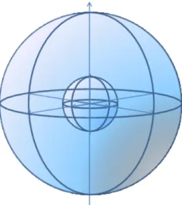
sphere can be chosen independently from the radiusRused for the computation of the local reference frame, but in our solution we considered the spherical support as having the same radiusRused for the computation of the reference frame (i.e., 15 mm in our setting). This spherical volume is then divided along three dimen-sions:radial,azimuthalandaltitude.
Along the radial dimension, the sphere is divided into con-centric shells. To avoid the quadratic growth of the shell volumes with the shell index, a logarithmic parametrization of the shell radii is used ri¼ 1 s loga as i s ; ð6Þ
whereriis the radius of the shell of indexi,s is the number of
shells, and a is a parametrization coefficient that controls the growth of the shell radius (e.g., for a¼1 the growth is linear, whereas with a¼2 the volume of the shell is kept constant at different radius). The shells are then divided in the azimuthal plane using sectors of constant angular width, and along the elevation. In the experiments reported in Section 5, we used a¼2, with three shells, four azimuthal sectors and two divisions along the elevation angle, resulting in a coarse partition of the volume around the keypoint into 24 spatial regions.Fig. 3shows the idea of the volumetric partitioning of the spherical space around a keypoint (for the clarity of the plot just two shells are reported).
Once the local support is partitioned into volumetric regions (based on the unique 3D local reference frame), the histogram of the normals of the mesh vertices within the support is used as local descriptor (called SHOT in [53]). This histogram based representation provides the filtering effect required to achieve robustness to noise, and enhances the discriminative power of the descriptor by introducing geometric information about the loca-tion of the vertices within the support. Asfinal step, all the local histograms are grouped together to form the signature which describes the mesh at the keypoint.
For each of the local histograms, mesh vertices contribute to bins according to a function of the angleθi, formed by the normal
at each vertex within a volume of the support partition,nvi, and
the normal at the keypoint,nu. The cosθifunction is used, in that
it can be computed efficiently using the dot product (i.e., cosθi¼nunvi), and equally spaced binning on cosθiis equivalent
to a spatially varying binning onθi. This latter property results in a
coarser binning for directions close to the reference normal direction and afiner one for orthogonal directions. In this way, small differences in orthogonal directions to the normal that are the most informative ones, cause a vertex to be accumulated in different bins and thus leading to different histograms. Instead, in the presence of quasi-planar regions this choice limits histogram differences due to noise by concentrating the contributions of the vertices in a fewer number of bins. In our experiments, we used 10 bins for each local histogram that combined with the partition into 24 volumetric regions, that results in a 240-dimensional signature for the keypoint.
To avoid boundary effects in the local histograms due to small differences of the spatial subdivision of the support, or to pertur-bations of the local reference frame, each vertex contributes to four histogram bins according to a quadrilinear interpolation between neighbors bins. In particular, the neighbor bins are represented by the neighboring bin in the local histogram and the bins having the same index in the local histograms of the neighboring volumes of the spatial partition. In doing so, each vertex contributes to neighbors bins by the weight 1−d, where for the local histogram,dis the distance of the current entry from the central value of the bin; for elevation and azimuth dimensions,dis the angular distance of the entry from the central value of the closer volume along the dimension; for the radial dimension,dis the Euclidean distance of the entry from the central value of the closer volume along the radial dimension. Along each dimension,d is normalized by the distance between two neighbor bins or volumes. Finally, to achieve robustness to variations of the vertex density, all the local histograms are concatenated into a whole descriptor (signature) which is further normalized to sum up to 1, so as to retain the local differences as a source of discriminative information.
The local signature at a generic keypoint is expressed through a normalized histogram G¼ ðg1;…;gNÞ where the size N of the
signature depends on the size of the local histograms and on the number of volumes of the partition (i.e., the quantization along the radial, azimuthal and elevation dimension) of the local reference frame (N¼240 in our case). Given two signatures G¼ ðg1;…;gNÞ
andH¼ ðh1;…;hNÞextracted at two keypoints, their dissimilarity
is measured through theChi-squaredistanceχ2, given by
χ2ðG;HÞ ¼1 2 ∑ N n¼1 ½gn−hn2 gnþhn : ð7Þ
The Experiment 2 Code Item 2 can be executed on the Experiment 2 Data Item 1, in order to generate the SHOT signature of a 3D face scan.
3.3. Multi-ring geometric histogram
The geometric histogram (GH) is a local geometric descriptor proposed by Ashbrook et al.[55]and employed in surface align-ment and matching. Basically, it is a 2D accumulator, or frequency table that counts the frequencies of two geometrical measure-ments, namely the angle and the distance between pairs of facets in a given neighborhood of a keypoint. In the following, we propose and describe a variation of the GH, which resulted more suited to our framework. This variant, develops on the idea of constructing the GH descriptor at a given keypoint in an incre-mental way, by accounting for an ordered sequence of rings defined around the keypoint. This idea is illustrated through the two steps involved in the computation: Derivation of theordered ring facetsin the neighborhood of the keypoint; Construction of thediscrete distributionsin each ring. In doing so, it is relevant to note that the GH descriptor is robust to translations and rotations also avoiding the computation of a reference frame.
Fig. 3.Spherical local support around a keypoint. The volumetric partition of the sphere along the radial, azimuthal and elevation dimensions is reported.
Ordered ring facets. The Ordered Ring Facets (ORF)[56] is the method used to identify the facets of the mesh which are comprised in the neighborhood of a keypoint. In this approach, the neighbor-hood construction around a central facettcis performed through a
sequence of concentric rings of facets emanating from a root facet (i. e.,tc). The facets are arranged circular-wise within each ring. The size
of the neighborhood is simply controlled by the number of rings. This mechanism allows an easy analysis of the GH variability, and thus of the local geometry evolution, as the size of the neighborhood increases. When the triangular mesh is regular and the facets are nearly equilateral, the ORF rings form an approximation of iso-geodesic rings around the central facettc. The ORF construction has
a linear complexity.Fig. 4depicts examples of ORF's with increasing number of rings and their related GH's. In the experiments reported inSection 5, we obtained good results by using 8 ORF as neighbor-hood of the keypoints.
Discrete distribution. Consider a triangular mesh approximation
^
S¼ ft1;…;tMg of an object surface. The discrete geometric
dis-tribution is constructed for each triangular facettiin a given mesh
which describes its pairwise relationship with each of the other surrounding facets within a predefined neighborhood. The range of the neighborhood controls the degree to which the representa-tion is a local descriprepresenta-tion of shape. Here, we choose a neighbor-hood range that encompasses the facets that share one or two vertices with the central triangular facet (Fig. 5(b)). The distribu-tion is defined such that it encodes the surrounding shape geometry in a manner which is invariant to rigid transformations of the surface data and which is stable in the presence of surface clutter and missing surface data.
Fig. 5(a) shows the measurements used to characterize the relationship between facettiand one of its neighboring facetstj.
These measurements are the relative angle,α, between the facet normals, and the range of perpendicular algebraic distances,d, from the plane in which facettilies to all points on the facettj. The
range of perpendicular algebraic distances is defined by½dmin;dmax,
where dmin and dmax are the minimal and the maximal of the
distance from the plane, respectively, in whichtilies to the facettj.
These extreme entities are simply obtained by calculating the
Fig. 4.ORF neighborhoods with different sizes constructed at a facial keypoints near to the nose, and their corresponding GHs.
Fig. 5.(a) The geometric measurements used to characterize the relationship between two facetstiandtj. (b) A facett1and its neighbor facets. (c) For each pair ðt1;tsÞ;s¼1;…;10, the angleαbetween the two facets'normals, the minimal and the maximal of the perpendicular distance from the plane oft1to the facettsare computed. (d) The pairs (α;d) derived from these measurements are entered in a 2D accumulator, obtaining thus a geometric distribution that characterizes the relationship between the facett1and its neighbors. (e) The geometric distribution can be visualized with a gray level mapping.
distances to three vertices of the facettjand then selecting the
minimal and the maximal distances.
Since the distance measurement is a range rather than a single value, from each measurement ðα;dmin;dmaxÞ can be derived a
number of measurements ðα;dÞ (dmin≤d≤dmax). This number
depends on the amplitude of the range½dmin;dmaxand the resolution
adopted for the distance parameter d. The group of pairs ðα;dÞ, extracted from the measurements related to a given facet and its neighbors (Fig. 5(b) and (c)), are entered to a 2D discrete frequency accumulator that encodes the perpendicular distancedand the angle
α(Fig. 5(d)). This accumulator has sizeNM;whereNandMare the number of bins in the axisαandd, respectively. The values of the accumulated matrix are also normalized so as to sum up to 1. The accumulator can be visualized in a 2D plotting using a gray level colormap (Fig. 5(e)), and stored in a matrix for subsequent processing. This representation only depends upon the surface shape and not on the placement of facets over the surface. This independence on the placement of the facets is important as it guarantees the invariance of the correspondence with respect to geometric transformations. A possible variant of the geometric histogram is obtained by consider-ing all the pairs of facets within Ntc, i.e., the set fðti;tjÞ; ti∈Ntc;
tj∈Ntcg. The construction of this variant is computationally more
demanding as the number of histogram entries evolves quadratically with respect to the number of facets in the neighborhood. Due to this, in our experiment we considered the computation referred to the central facettc, usingN¼8 andM¼20.
With respect to the computation of the central GH, we introduced a variant which is related to the ORF definition. In particular, in our approach, a GH is constructed on each of the rings that constitute the ORF of a keypoint: This means that the GH descriptor is actually given by a set of GH, constructed on the sequence of rings which surround the keypoint. This improves the descriptiveness of GH by capturing information on how the local characteristic of the surface changes when the distance from the keypoint increases. This multi-ring structure is also exploited during the match. In particular, the normalized GH can be viewed as a probability density function, and thus can be adapted to probabilistic matching paradigms. To this end, the Bhattacharyya distance (dB) is used as metric for evaluating the similarity
between GHs at each ring. According to this, given two GHs in the form of 1D arrays ofK¼NMelements,AðlÞ ¼ fa1;…;aKgand
BðlÞ ¼ fb1;…;bKg, their distance at ring-l is computed as
dBðAðlÞ;BðlÞÞ ¼ ffiffiffiffiffiffiffiffiffiffiffiffiffiffiffiffiffiffiffiffiffiffiffiffiffiffiffiffiffiffiffiffiffiffiffiffiffi 1− ∑K k¼1 ffiffiffiffiffiffiffiffiffiffiffiffiffiffiffiffi ðakbkÞ p s : ð8Þ
The overall distance between two multi-ring GH, computed onL rings is then obtained by accumulating the distances between the GHs at different rings, that is
dðA;BÞ ¼ ∑L
l¼1
dBðAðlÞ;BðlÞÞ: ð9Þ
The Experiment 2 Code Item 2 can be executed on the Experiment 2 Data Item 1, in order to generate the GH descriptor of a 3D face scan.
4. Face matching
Given two face scans, their comparison is performed by matching the local shape descriptors at corresponding keypoints under the constraint that a consistent spatial transformation exists between inliers pairs of matching keypoints. To this end, local shape descriptors at the keypoints detected in probe and gallery scans are compared so that for each keypoint in the probe, a candidate corresponding keypoint in the gallery is identified. In particular, a keypointkpin the probe is assigned to a keypointkgin
the gallery, if they match each other among all keypoints, that is, if and only if kp is closer to kg than to any other keypoint in the
gallery and kg is closer to kp than to any other keypoint in the
probe. For this purpose, distance between keypoints descriptors is measured through the distances presented for the three local descriptor HOG, SHOT and GH, discussed, respectively, inSections 3.1–3.3. Finally, the candidate matches for which the second best match is significantly worse are accepted (i.e., a match is accepted if the ratio between the distance of the best match and the second best match is lower than 0.7).
This analysis of proximity of keypoint descriptors results in the identification of a candidate set of keypoint correspondences. Identification of the actual set of keypoint correspondences must pass afinal constraint targeting the consistent spatial transforma-tion between corresponding keypoints in the probe and gallery scans. The RANSAC algorithm [43,57] is used to identify outliers in the candidate set of keypoint correspondences. This involves generating transformation hypotheses using a minimal number of correspondences and then evaluating each hypothesis based on the number of inliers among all features under that hypothesis. In our case, we modeled the problem of establishing correspondences between sets of keypoints detected on two matching scans as that of identifying points inR3that are related
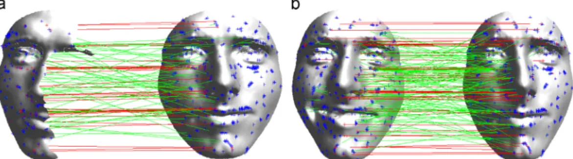
via a rotation, scaling and translation transformation (RST trans-formation). According to this, at each iteration, the RANSAC algorithm validates sampled pairs of matching keypoints under the current RST transformation hypothesis, updating at the same time the RST transformation according to the sampled points. In this way, corresponding keypoints whose RST transfor-mation is different from thefinal RST hypothesis are regarded as outliers and are removed from the match. Examples of the application of RANSAC are reported inFig. 6. In thefigure, detected keypoints are highlighted with a“+”symbol (in blue); correspond-ing keypoints based on descriptors matchcorrespond-ing are connected by green lines;finally, the inliers matching which pass the RANSAC algorithm are shown with a red line connection. It can be observed as by applying the RANSAC algorithm just the matches that show a coherent RST transformation among each other is retained. This avoids matches of keypoints that are located in different parts of the face of two scans. Cases in (a) and (b), respectively, report the match between two scans of the same subject and of different subjects. InFig. 7, we also report the case in which scans of the same subject with large missing parts (a) and with expression (b) are matched against a full neutral gallery scan. It can be observed as the number of inliers is still high compared to that of different subjects, despite the large missing parts and expression.
Once the set of inlier keypoints is established, the distance between their descriptors is accumulated and averaged. Given a probe and a gallery, the correspondences identified by the spatial transformation hypothesis is a function ξ:ℵ↦ℵ that associates with a keypoint descriptor CðpÞ
k in the probe, its corresponding
keypoint descriptorCðgÞ
ξðkÞin the gallery. For each keypoint
descrip-tor in the probeCðpÞ
k the distance to the corresponding keypoint
descriptorCðgÞ
ξðkÞin the gallery is evaluated (using Eq.(7)for SHOT or
Eq. (9) for GH), and these distances arefinally averaged on the total number of inlier matchesNi
D¼ 1 Ni ∑ Ni k¼1D ðCðpÞ k ;C ðgÞ ξðkÞÞ: ð10Þ
In this way, the distance between two face scans is regarded as a pair〈Ni;D〉. The number of matching inliers is used as measure of
distance. In the case two scans have the same number of inliers, the distanceDserves as disambiguation value.
The Experiment 3 Code Item 2 can be executed on the Experiment 3 Data Item 1 and Experiment 3 Data Item 2, in order to compute the match between two 3D face scans using local descriptors and RANSAC. An image showing the keypoints match-ing is also generated.
About the computational complexity of the proposed matching approach, it depends on two main cost factors: the matching of local descriptors and the execution of the RANSAC algorithm. The
first term resulted the main source of cost, growing quadratically with the number of keypoints in the two scans. All the three descriptors presented inSection 3are histogram based and so the complexity in computing their match depends on the distance measure and on the number of histogram bins.
5. Experimental results
The performance of the proposed approach has been evaluated in a comprehensive set of experiments. For the sake of the presentation and discussion, experiments have been divided and organized into two parts:
1. The goal of thefirst session of experiments was to evaluate the robustness of our 3D face recognition solution to probes showing large facial expressions (from moderate to exagger-ated), and extreme pose variations (side rotations of 901). To this end, experiments were carried out on two datasets that are specifically designed for investigating 3D face recognition in the presence of facial expressions, The Binghamton University 3D Facial Expression database (BU-3DFE) [44], and missing parts,The 2D/3D Florence Face dataset(UF-3D)[45]. In addition, we provide an in depth investigation on the keypoints detec-tion and repeatability, using the same datasets. Results of this
first session of experiments are reported inSection 5.1.
2. In the second session of experiments, the proposed approach is evaluated on a variety of benchmark datasets that differ in the number of scans, acquisition modalities and characteristics of the scans in terms of missing parts, occlusions, and expressions. The used databases are theBosphorus[28],Gavab[14]andUND/ FRGC v2.0[6]. These datasets have been used by many of the existing 3D face recognition works, thus permitting a direct comparison of our approach with state of the art solutions.
Section 5.2reports results of this evaluation.
The datasets listed above largely differ in the scanners used during acquisition (i.e., either laser or structured light scanners), so that both 2.5D (only onez-value is possible at a givenxylocation) and 3D acquisitions are involved (multiplez-values at the samexy location are allowed). According to this, in the perspective of not to restrict the proposed approach to any particular scenario, in the experimentation we do not make any assumption about the type of scans available in the probe or gallery sets (i.e., they can be either 2.5D or 3D).
5.1. Performance evaluation
The objective of the results reported in this section is to verify the performance of the proposed approach in the case of probes with very large facial expressions (Section 5.1.1), and extreme side rotations (Section 5.1.2). In so doing, we devised anidentification scenario where the effectiveness of recognition is measured through the rank-k recognition rate (RR): a rank-k recognition experiment is successful if the gallery face representing the same individual of the current probe is ranked within the first k positions of the ranked list. The rank-1 value has been reported in our experiments.
Fig. 7.(a) Partial probe vs. full gallery same subject (34 inliers). (b) Expressive probe vs. neutral gallery same subject (47 inliers). (a) same subject: missing parts and (b) same subject: expression.
Fig. 6.Matching of scans of same and different subjects are reported in (a) and (b), respectively. All the detected keypoints are shown with“+”. Lines indicate matching keypoints (in green), and inliers matching after RANSAC (in red). In the case of scans of the same subject in (a), 61 inlier matches are identified; For scans of different subjects in (b), 18 matches are detected. (For interpretation of the references to color in thisfigure caption, the reader is referred to the web version of this article.)
5.1.1. The BU-3DFE database
The BU-3DFE database was recently constructed at Binghamton University[44]. It has been designed to provide 3D facial scans of a large population of different subjects each showing a set of facial expressions at various levels of intensity. There are a total of 100 subjects in the database, divided between female (56 subjects) and male (44 subjects). The subjects are well distributed across different ethnic groups or racial ancestries, includingWhite,Black,East-Asian, Middle-East Asian,Hispanic-Latino, and others. During the acquisition, each subject was asked to perform the neutral facial expression as well as the six basic facial expressions defined by Ekman [58], namely anger,disgust,fear,happiness,sadness, andsurprise. Each facial expres-sion has four levels of intensity, respectively low, middle,high and highest, except the neutral facial expression that has only one intensity level. Thus, there are 25 3D facial expression scans for each subject, resulting in 2500 3D facial expression scans in the database. As an example,Fig. 8shows the 3D scans of a sample subject showing the six basic facial expressions at thelowandmediumlevels of intensity.
Face recognition results. The BU-3DFE dataset has been used to investigate the robustness of the proposed approach with respect to facial expressions in a wide range of intensity variations, from low to exaggerated. This allowed us to infer some evidence of the facial variations that mostly affect face recognition. So far, the BU-3DFE database has been used mainly to test facial expression recognition methods, rather than the robustness of face recogni-tion methods in the presence of expression variarecogni-tions. Actually, face recognition experiments on the BU-3DFE were conducted in
[59,60], but only cumulated results were reported in these works, without a detailed analysis for each expression/intensity. As a consequence, for the large part of the methods reported in the literature, there is no insight of the effect induced by different expressions.
In our experiments, we randomly partitioned the dataset into a training and a testing set. The scans of 20 subjects have been included in the train set and have been used for tuning the parameters of the
3D keypoints detector (i.e., the number of DOG scales, the percentage and cornerness thresholds, seeSection 2) and the local descriptors (i.e., number of histogram bins for HOG, SHOT and GH descriptors, see
Section 3). A classic grid search approach has been used to this end (this phase is mainly important for keypoints detection, since the percentage and cornerness thresholds largely influence the number of detected keypoints, which can vary of an order of magnitude or so). These parameters have been used in the experiments carried out on this dataset, on the UF-3D database (as reported in the next section) and on the three databases used in Section 5.2. The scans of the remaining 80 subjects have been included in the test set. In particular, we considered the neutral scan of each subject as a reference scan and included it in the gallery set (gallery with 80 neutral scans in total). The probe set is composed of 24 expressive scans for each subject, including for each expression the scans with low,medium highand highestintensity level (seeFig. 8). With this selection, the probe set includes 1920 expressive probe scans. The scans classified as showing a lowand mediumexpression intensity have moderate and natural expressions, similar to those that are likely to occur in a real context. Instead, scans classified in the BU-3DFE as havinghighand highest expression intensity, present quite exaggerated expressions for the large part of the subjects, and are more suited to verify the perfor-mance of the approach in very difficult situations.
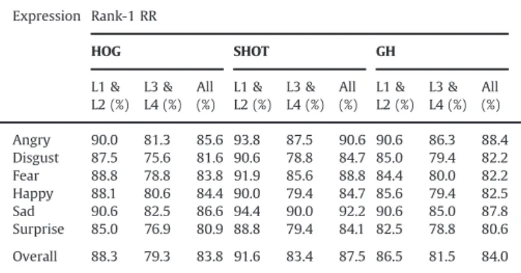
Using these probe and gallery sets, we performed recognition experiments based on keypoints matching with each of the three local descriptors presented in Section 3. Rank-1 recognition accuracies are reported inTable 1, separately for the six expres-sions, and for the low and medium intensity level (L1 & L2), and the high and highest level (L3 & L4). From the table, it can be observed that, as the overall performance is concerned, the SHOT descriptor provides the best results among the three local descrip-tors. Looking in to the performance of the SHOT descriptor, it results that the expression that makes the recognition more difficult is thesurpriseone at L1 & L2. This is confirmed also using the HOG and GH descriptors. This is mainly due to the open mouth
that appears in the large part of subjects with this expression. The effect of this is a modification of both the location of the detected keypoints with respect to the neutral case, as well as a change of the local descriptors. At L3 & L4 also faces withdisgusted expres-sion become difficult to be recognized. Furthermore, from this analysis also results that the performance with the GH descriptor seems to degrade more gracefully than for the other descriptors when passing from L1 & L2 to L3 & L4.
5.1.2. The 2D/3D Florence face dataset
The 2D/3D Florence face dataset (UF-2D/3D)1 has been
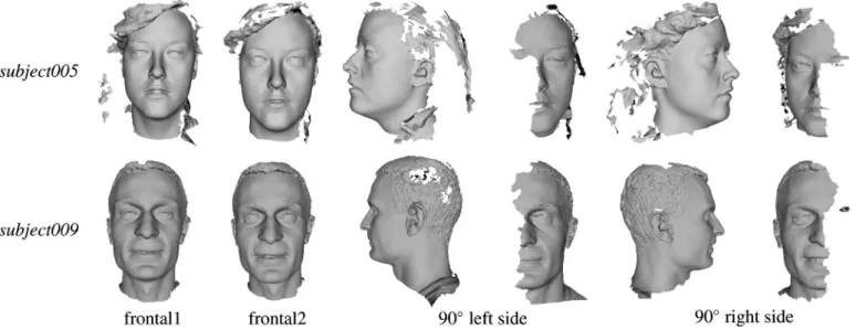
con-structed at the Media Integration and Communication Center of the University of Florence[45]. The dataset consists of high-resolution 3D scans of human faces along with several video sequences of varying resolution and zoom level. This dataset is designed to simulate, in a controlled fashion, realistic surveillance conditions and to test the efficacy of exploiting 3D models in real scenarios. In this work, we used the 3D part of the dataset (UF-3D) that currently includes 53 subjects (14 females and 39 males, numbered from subject001 to subject053) of Caucasian ethnicity. The age of the subjects ranges from 20 to 60, with the majority of the subjects (28) being student at the School of Engineering of the University of Florence, aged between 20 and 30 years. The 3D scans of each subject are acquired in the same session and include two frontal scans with neutral expression (named asfrontal1andfrontal2), and two scans where the subject is rotated of 901on the left and right sides (namedleftandright, respectively). In all the acquisitions, the subjects are required to assume a neutral expression, though some scans exhibit moderate, involuntary, facial expressions. The3dMD face system[10]scanner has been used in the acquisition, which produces one continuous point cloud from two stereo cameras with a capture speed of about 1.5 ms at the highest resolution, and a geometry accuracy lower than 0.2 mm RMS. As an example,Fig. 9reports the 3D face scans of two sample subjects.
Face recognition results. The UF-3D dataset allows us to evaluate the recognition accuracy of the proposed solution in the case of frontal neutral probes as well as for probes with extreme yaw rotations. In particular, the left and right probes in this dataset have been acquired with side rotation of 901, which results in scans with half of the face missing, with consequent very challen-ging recognition conditions. One neutral scan (“frontal1”) has been selected as reference for each subject and included in the gallery.
The other neutral scan of each subject (“frontal2”) has been used as probe in the“neutral vs. neutral”experiment. The left/right scans have been used in two separate experiments aiming to test the robustness of the proposed approach to partial face matching, where large parts of the face are missing. It is relevant to note that being the proposed approach based completely on 3D processing, both keypoints detection and local description extraction can be performed without the need of costly pose normalization solu-tions that are required by other existing methods[23,24,29,35].
Results of this evaluation are reported in Table 2. It can be observed that the proposed solution achieves a very high accuracy in matching neutral frontal scans, with each of the three experi-mented descriptors showing a similar behavior (in this case the SHOT descriptor achieves the best results). For side scans, the accuracy drops significantly with similar results obtained for the left and right scans. The GH descriptor evidences the highest accuracy in this experiment. To the best of our knowledge, the only two other works reporting results on probes with yaw rotations of 901 are those in [36,46], though these two approaches were experimented on the Bosphorus database. Direct comparison of our solution with respect to[36,46] on the Bosphorus database is given inSection 5.2.1.
Fig. 10 shows two examples of wrong recognition for probes with large missing parts. In both the cases, the number of inliers resulted too low to allow rank-1 recognition. For the case on the left, this can be motivated by the presence of a facial expression (see the open mouth) which is combined with a large part of the face missing. In the case on the right, the main problem was originated by the preprocessing operation, which closes holes in the face scans. Due to the large extent of the hole, the holefilling procedure fails in producing a consistent closing, thus altering the face geometry and the keypoints extraction and description.
5.1.3. Localization and repeatability of 3D keypoints
The idea of representing the face by a sparse and adaptive set of automatically detected keypoints relies on the assumption of intra-subject keypoints repeatability: Keypoints extracted from different facial scans of the same individual are expected to be located approximately in the same positions of the face. Since keypoints detection only depends on the geometry of the face surface through its mean curvature (see Section 2), these key-points are not guaranteed to correspond to specific meaningful landmarks of the face. For the same reason, the detection of keypoints on two face scans of the same individual should yield to the identification of the same points of the face, unless the shape of the face is altered by major occlusions or non-neutral facial expressions.
To test the repeatability of keypoints detection, we used the 3D scans of the BU-3DFE database selected for the experiments reported inSection 5.1.1. We followed the approach proposed in
[31], and measured the correspondence of the location of key-points detected in two face scans by performing ICP registration. Accordingly, the 3D faces belonging to the same individual are automatically registered and the errors between the nearest neighbors of their keypoints (one from each face) are recorded.
Fig. 11shows the results of our keypoint repeatability experiment, by reporting the cumulative rate of repeatability as a function of increasing values of the distance. The repeatability reaches a value of 90% for frontal faces with neutral and non-neutral expressions at a distance error of 5 mm (with an average number of 360 keypoints detected per scan). We remark that these results, and those reported in the following about the number of detected keypoints, have been obtained by computing 96 DOG scales, and retaining the unique keypoints that are detected in the last 64 DOG scales (see alsoSection 2).
Table 1
BU-3DFE: rank-1 recognition rate (RR) for different expressive scans. Results are reported separately for the HOG, SHOT and GH descriptors. For each descriptor, the average for thelowandmediumexpression intensity (L1 & L2), and for thehighand
highestintensity level (L3 & L4) are reported, together with the average on all the intensity (Allcolumn).
Expression Rank-1 RR HOG SHOT GH L1 & L2 (%) L3 & L4 (%) All (%) L1 & L2 (%) L3 & L4 (%) All (%) L1 & L2 (%) L3 & L4 (%) All (%) Angry 90.0 81.3 85.6 93.8 87.5 90.6 90.6 86.3 88.4 Disgust 87.5 75.6 81.6 90.6 78.8 84.7 85.0 79.4 82.2 Fear 88.8 78.8 83.8 91.9 85.6 88.8 84.4 80.0 82.2 Happy 88.1 80.6 84.4 90.0 79.4 84.7 85.6 79.4 82.5 Sad 90.6 82.5 86.6 94.4 90.0 92.2 90.6 85.0 87.8 Surprise 85.0 76.9 80.9 88.8 79.4 84.1 82.5 78.8 80.6 Overall 88.3 79.3 83.8 91.6 83.4 87.5 86.5 81.5 84.0
1The database is publicly available and can be accessed upon request from the
following address:http://www.micc.unifi.it/masi/research/ffd/. The dataset is also released within the Elsevier Collage Authoring Environment.