PARTICLE-BASED STOCHASTIC REACTION-DIFFUSION MODELS TO INVESTIGATE SPATIOTEMPORAL DYNAMICS IN CELL BIOLOGY
Vinal Vinodrai Lakhani
A dissertation submitted to the faculty at the University of North Carolina at Chapel Hill in partial fulfillment of the requirements for the degree of Doctor of Philosophy in the Curriculum
of Bioinformatics and Computational Biology
Chapel Hill 2015
Approved by:
ii © 2015
iii ABSTRACT
Vinal Vinodrai Lakhani: Particle-Based Stochastic Reaction-Diffusion Models to investigate Spatiotemporal Dynamics in Cell Biology
(Under the direction of Timothy Elston)
Many facets of mathematics, science and engineering rely on numerical methods to study complex systems, for which analytical methods fail. For example, in particle-based models the positions of individual particles under the influence of various forces are monitored over time. These models are used to study phenomena ranging from the structure and dynamics of galaxies (where particles represent stars) to proteins (where particles represent atoms). In this document, we present two applications of particle-based modeling to study microscopic dynamics in cell biology, which would otherwise be invisible by current experimental methods. In both models, the particles represent protein molecules, and we calculate the stochastic biochemical reactions and diffusion of tens of thousands of proteins over time. We utilize Generally Programmable Graphics Processing Units (GPGPUs) to achieve the high performance computing necessary to simulate these large scale models.
Chapter 1 begins with the observation that the mobility of Rac1 molecules, which are important regulators of the cell cytoskeleton, is spatially regulated in migrating cells.
Specifically, Rac1 molecules near the leading edge have less mobility than those in the trailing edge. We create a particle-based stochastic reaction-diffusion model to test the hypothesis that patches of actin, called ‘actin islands’, are responsible for this observation. We find that these islands are capable of producing the spatially-dependent mobility measured by in vivo
iv
v
vi
ACKNOWLEDGEMENTS
This document is the culmination of the hard work of many people. First and foremost is my fantastic mentor: Tim. On an educational level, Tim opened my eyes to world of Systems Biology, which looks at the world as a network of connections and interactions. And although this field can be incredibly daunting, Tim showed me the power of simplification. He taught me to consider only the minimal set of components capable of answering the question. He taught me that good science starts this way and adds only one variable at a time. But one of the biggest impacts Tim’s tutelage had on me was to motivate and excite me. There were times during my project when I felt discouraged about my results or my lack of progress; but each time I met with Tim, he would find exciting questions and opportunities with the results I DID manage to get. His excitement always spurred me forward, feeling undaunted and eager to answer new
questions. Lastly, I cannot stress enough the patience Tim had with me. He was patient with me as I debugged my code and as I struggled to understand the confusing results. Most importantly he was patient with me when my progress slowed due to difficulties in my family life.
vii
Patrick McCarter, Lior Vered, Maria Minakova, Conner Sandefur, Ellen O’Shaughnessy, and Alex Chen, for their emotional and intellectual encouragement. I can recall conversations with each member wherein they taught me about yeast biology, gave me great ideas about my model, or brainstormed new ideas.
Tim and I also had the pleasure of collaborating with Drs. Enrico Gratton and Elizabeth Hinde from the Laboratory of Fluorescence Dynamics at UC Irvine. Liz performed the
experiments and generated the pCF carpets for her experimental data and my simulations. Our work is presented in Chapter 1.
I must also thank my friends: Michael Zytkow, Lawrence Ngo, Cameron Smith, Devin Hubbard, and Zack Cashion, for dreaming big and encouraging me to do the same. I am indebted to the Hubbard family for their unmatched kindness and support. And finally, I thank the
Lakhani family, who raised me and instilled in me a great respect for education. I am grateful for every conversation with my cousins, who, even today, remain invaluable sources of knowledge and intellectual discourse. Finally, although we’ve only been married for three months, Krupal has patiently supported, encouraged, and pushed me through this ultimate phase of my education. As Tim put it, when I told him that I was getting married, he replied “Now you have motivation to finish.”
viii
TABLE OF CONTENTS
LIST OF TABLES ... xi
LIST OF FIGURES ... xii
CHAPTER 1: SPATIO-TEMPORAL REGULATION OF RAC1 MOBILITY BY ACTIN ISLANDS ... 1
Introduction ... 1
1.1 Overview ... 1
1.2 Intracellular Traffic Observed in in silico simulations by Pair Correlation Analysis ... 5
1.3 Gradient of Molecular Flow Observed in in vivo experiments by Pair Correlation Analysis ... 7
1.4 Gradient of Rac1 Molecular Flow Produced by Actin Island Simulations ... 10
1.5 Discussion ... 14
1.6 Methods ... 17
1.6.1 Simulation Algorithm ... 17
1.6.2 Pair Correlation Carpet ... 22
1.7 Supplemental Methods ... 24
1.7.1 Analyzing pCF Carpets ... 24
1.7.2 Simulation Program Details ... 25
1.7.3 Calculating Diffusion Steps ... 25
1.7.4 Calculating Reaction Probabilities ... 29
ix
1.7.6 Generating an Intensity Carpet ... 35
1.7.7 Hardware Details ... 35
References ... 37
CHAPTER 2: A MODEL OF GRADIENT SENSING IN THE CONTEXT OF YEAST MATING ... 38
Introduction ... 38
2.1 Overview ... 39
2.2 Binding Reactions ... 41
2.3 Unbinding Reactions ... 43
2.4 Diffusion of Pheromone ... 43
2.4.1 Pheromone Gradient – Method 1 ... 44
2.4.2 Pheromone Gradient – Method 2 ... 46
2.5 Diffusion of Receptors ... 47
2.6 Algorithm Overview ... 48
2.7 Receptor Cycling Model ... 49
2.8 Bar1 Model ... 50
2.9 Calculating Binding Probability ... 51
2.10 Calculating Pheromone Reflection off the Cell Surface ... 56
2.11 Injection Boundary Condition: Derivation of Eqs 2.5 – 2.8 ... 58
2.11.1 Gradient Method 1 ... 59
2.11.2 Injection Distance ... 61
2.11.3 Gradient Method 2 ... 64
2.12 Receptor Diffusion on the Cell Surface: Derivation of Eq 2.9 ... 66
x
References ... 68
CHAPTER 3: USING STOCHASTIC SIMULATIONS TO ASSESS NOISE-REDUCTION MECHANISMS DURING GRADIENT SENSING IN YEAST ... 70
Introduction ... 70
3.1 Background ... 71
3.2 Overview ... 75
3.3 Equilibrium Fluctuations in Uniform Pheromone ... 76
3.3.1 Equilibrium Fluctuations in Receptor Occupancy ... 76
3.3.2 Time Averaging ... 78
3.3.3 The “Perfectly Absorbing” Cell and Receptor Cycling ... 82
3.4 Cells at Equilibrium in a Pheromone Gradient ... 85
3.4.1 Gradient Sharpening due to Steric Effects ... 85
3.4.2 Slow Reaction Rates and Receptor Diffusion add Spatial Noise ... 87
3.4.3 Time-averaging and the Angle of Estimation ... 89
3.5 Sensing During Gradient Formation ... 92
3.5.1 Formation of the Gradient ... 92
3.5.2 Transient Differences in Receptor Occupancy ... 93
3.5.3 Bar1 Improves Gradient Sensing for Fast Reaction Rates ... 96
3.6 Discussion ... 97
3.6.1 Mechanisms for Noise-Reduction ... 97
3.6.2 Gradient Sharpening due to Steric Effects ... 98
xi
LIST OF TABLES
xii
LIST OF FIGURES
Figure 1.1 – Pair correlation analysis of a fluorescent protein’s diffusive
route reveals how the cell’s architecture directs intracellular traffic ... 4
Figure 1.2 – Pair correlation analysis of a Rac1 FRET biosensor reveals Rac1 activity to be spatiotemporally regulated by a dynamic gradient of protein mobility ... 9
Figure 1.3 – Simulations with islands of varying binding affinity ... 11
Figure 1.4 – Investigating the cellular substructure during three stages of EGF stimulation by comparing pCF carpets ... 13
Figure 1.5 – Simulation Geometry ... 19
Figure 1.6 – Gaussian Analysis of Pair Correlation Carpets to Extract Average Delay Time(s) Rac1 Takes to Diffuse Along Simulated and in vivo Line Scans ... 24
Figure 1.7 – Important Vectors for Reflecting Inside Actin Islands ... 27
Figure 2.1 – Simulations on our Particle-Based Stochastic Reaction- Diffusion Model ... 40
Figure 2.2 – Rationale for Doubling Pbind ... 56
Figure 2.3 – Reflecting Pheromone off Cell Surface ... 57
Figure 2.4 – Molecular Reservoir ... 60
Figure 2.5 – Injection Distance ... 61
Figure 2.6 – Probability Density of Injection Distance ... 63
Figure 2.7 – Cylindrical Bins ... 67
Figure 3.1 – Gradient Sensing during Yeast Mating ... 72
Figure 3.2 – Receptor Occupancy at Equilibrium ... 77
Figure 3.3 – Comparing Mathematical Models ... 80
Figure 3.4 – Uncertainty as a function of Time-Averaging ... 82
xiii
Figure 3.6 – Gradient Sharpening due to Steric Effects ... 85
Figure 3.7 – Receptor Occupancy in Linear Gradient vs Sharpened Gradient ... 87
Figure 3.8 – Receptor Diffusion adds Spatial Noise ... 88
Figure 3.9 – Estimated Angle away from Gradient ... 90
Figure 3.10 – Estimated Angle Improves with Time-averaging ... 91
Figure 3.11 – Cell’s Physical Boundary Sharpens an Emerging Gradient ... 92
Figure 3.12 – Initial, Transient Difference in Receptor Occupancy ... 93
1
CHAPTER 1: SPATIO-TEMPORAL REGULATION OF RAC1 MOBILITY BY ACTIN ISLANDS1
Introduction
Rho GTPases play important roles in many aspects of cell migration, including polarity establishment and organizing actin cytoskeleton. In particular, the Rho GTPase Rac1 has been associated with the generation of protrusions at leading edge of migrating cells. Previously it was shown that the mobility of Rac1 molecules is not uniform throughout a migrating cell (Hinde E et. al. PNAS 2013). Specifically, the closer a Rac1 molecule is to the leading edge, the slower the molecule diffuses. Because actin-bound Rac1 diffuses slower than unbound Rac1, we
hypothesized that regions of high actin concentration, called “actin islands”, act as diffusive traps and are responsible for the non-uniform diffusion observed in vivo. Here, in silico model
simulations demonstrate that equally spaced actin islands can regulate the time scale for Rac1 diffusion in a manner consistent with data from live-cell imaging experiments. Additionally, we find this mechanism is robust; different patterns of Rac1 mobility can be achieved by changing the actin islands’ positions or their affinity for Rac1.
1.1 Overview
Rho GTPases play a critical role in regulating many aspects of cell migration including polarity establishment and the actin cytoskeleton. Rac1 is a Rho GTPase associated with membrane protrusions at the leading edge of the cell [1]. Recent work demonstrated that Rac1 activity is closely regulated in space and time during the retraction portion of the
1 This chapter has been accepted for publication as an article in the PLoS ONE. It is titled “Spatio-temporal
2
retraction cycle. Specifically, Rac1 activity peaks 40 seconds after and 2 μm away from a protrusion event [2]. Previously, fluctuation analysis in polarized cells was used to establish that the time scale of Rac1 diffusion varied with its localization within the cell [3]. Using pair
correlation function (pCF) analysis, the time taken for a Rac1 molecule to move 1μm at each position along the axis of the cell was calculated [3]. In particular, a negative correlation between Rac1’s mobility and its proximity to the leading cell edge was found; Rac1 molecules took 100 times longer at the front of the cell than at the back to move 1μm [3]. These observations led to the hypothesize that diffusive barriers, such as those found in neurons for compartmentalizing proteins [4], are responsible for the observed spatial variation in diffusion. Here we use a computational model to demonstrate that diffusive barriers, in the form of “actin islands”, can establish gradients of molecular mobility across the cell similar to those observed for Rac1.
3
it was found that Rac1 mobility decreases near the leading edge of the cell where we also observe, by FRET analysis, Rac1 activity to be the highest [3]. We hypothesized that cells achieve this spatiotemporal control of Rac1 mobility by using patches of dense actin, we call “actin islands”, to which Rac1 reversibly binds. By strategically placing and adjusting the density of the actin in these actin islands, the cell can reduce mobility of Rac1 in the desired location. For example, to slow diffusion towards the leading edge, the actin islands can be denser towards the leading edge.
To test this hypothesis, we created a computational model to study Rac1 mobility within a cell containing actin-islands. Using a particle-based stochastic simulation algorithm, we explicitly simulate the diffusion of individual Rac1 molecules and their binding/unbinding reactions with actin-islands. Unbound Rac1 freely diffuses throughout the cell. The actin-islands behave as diffusive traps, capable of slowing the diffusion rate and restricting the accessible space for an actin-bound Rac1 molecule. During the simulation we tally the number of Rac1 molecules located in bins along the center axis of the cell. Analogously, in the in vivo
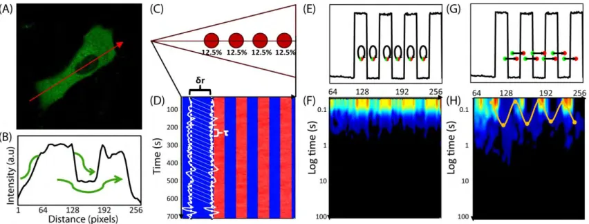
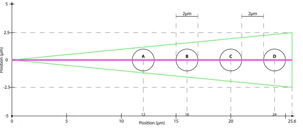
Fig. 1.1: Pair correlation analysis of a fluorescent protein’s diffusive route reveals how the cell’s architecture directs intracellular traffic.
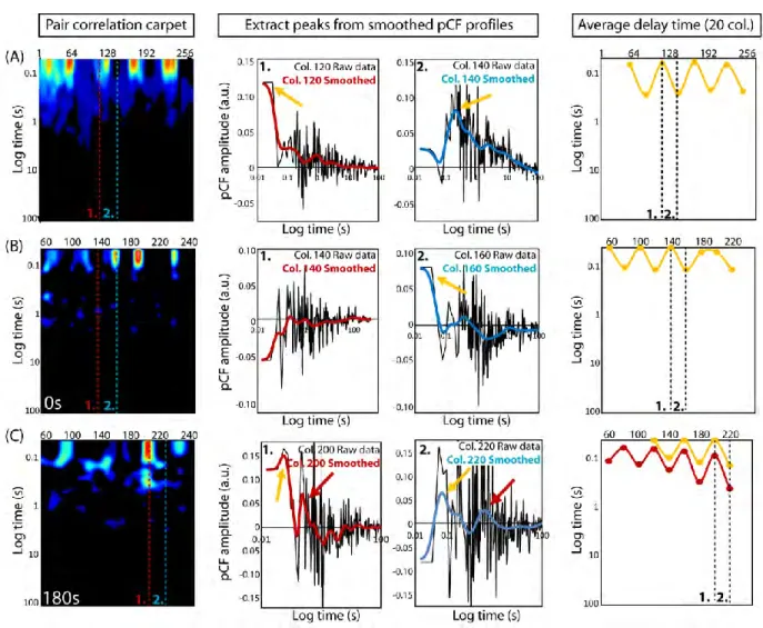
(A) Intensity image of cell expressing EGFP. Fluorescence data along the arrow is summarized in the next panel. (B) Intensity profile of 5-EGFP across axis of cell shows 5-5-EGFP exclusion from the nucleus and therefore an obstacle to 5-5-EGFP free diffusion. Green arrows demonstrate the molecules must diffuse around instead of through the obstacle. (C) Model for the simulation of Rac1 diffusion in a triangular shaped cell (25.6μm by 5μm) with four, circular traps (2μm wide). Each trap captures, on average, 12.5% of the total Rac1 population. Line scans are taken along the center axis of the cell, as shown by the horizontal line. Each pixel is measured in succession, and one line scan is completed when all 256 pixels have been measured. (D) Many (47000) line scans are combined into an intensity carpet. For this simulation, the intensity carpet shows accumulation of Rac1 colocalized with the four traps. A cartoon of two intensity profiles (intensity vs time) in white is overlaid on the intensity carpet. (E) A representative line scan (intensity vs pixel). The arrows indicate which two pixels are being pair-correlated, from green to red, for the pCF analysis in the next panel. In this case, each pixel is pair-correlated with itself, which is equivalent to an autocorrelation calculation. (F) The pCF(0) carpet reveals that pixels within the traps have higher autocorrelation values for short delay times (τ ≈ 0s) than pixels outside the traps. These values indicate the traps have a higher concentration of Rac1 than elsewhere in the cell. (G) The same representative line scan (intensity vs pixel) as in (E). Here the arrows indicate each pixel (green dot) is pair-correlated with a pixel (red dot) 0.5μm to the right (δr = 5 pixels). (H) The pCF(5) carpet reveals diffusion in and around the traps is slower than elsewhere in the cell. We average the data from every 20 pixels (columns) and smooth this average profile using a Gaussian filter; lastly, we extract the peak time for every 20 columns. We plot a point at each of these peak times. Hence, the yellow highlighted data displays the average time Rac1 takes to diffuse 0.5μm to the right. It takes about 0.3s to diffuse 0.5μm inside the islands but less than 0.1s to diffuse the same distance elsewhere in the cell.
5
1.2 Intracellular Traffic Observed in
in silico
simulations by Pair Correlation
Analysis
In live cells the default mechanism of motion for many biological molecules is diffusion. Although unregulated diffusion produces a spatially isotropic distribution of molecules, it is has been shown that structural features of the cell create intracellular compartments that generate spatially heterogeneous molecule distributions. For example, insights into intra-cellular trafficking have been derived from measuring the effect of the cell nucleus on the diffusion of biologically active and inert molecules [7]. The effect of the nucleus on diffusion is readily apparent, if we scan across the axis of an NIH3T3 cell transiently transfected with the
biologically inert fluorescent protein 5-EGFP (Fig. 1.1A). In this case, the fluorescence intensity profile clearly shows the exclusion of 5-EGFP from the nucleus (Fig. 1.1B). From this simple experiment we can deduce that the nuclear envelope behaves as an impenetrable barrier, around which 5-EGFP must diffuse. Given that intracellular trafficking of biologically active molecules is far more complex, the diffusive route traveled by a fluorescently labeled protein is not always evident from simple inspection of the fluorescence intensity distribution, and thus a more dynamic approach is required.
To gain insight into the diffusive motion active proteins, we employ an analysis method that is based on pairwise correlation functions. Using pairwise correlation analysis, it is possible to discern both diffusion rates and particle fluxes along a confocal line scan. These quantities are inferred by measuring temporal cross-correlations in fluorescence intensity between pairs of points a distance δr apart as a function of the time delay τ between measurements. To illustrate this idea consider the following in silico example. We simulate the diffusion of individual Rac1 molecules (D = 10μm2/s) inside a cell containing four diffusive traps (Fig. 1.1C). The cell is
6
molecules that diffuse into a trapping area can reversibly bind to the trap. When bound in a trap, Rac1 molecules are (1) spatially restricted to remain inside the trap, and (2) the diffusion
constant reduces to 1μm2/s. During the simulation we repeatedly take “line scans”, which are
measurements along a line that traverses the cell (Fig. 1.1C). Whereas the line scans for the in vivo experiments measured fluorescence intensity in each pixel (0.1μm)2 along the line, the line
scans for our in silico simulations measure the number of molecules in square bins (0.1μm)2
along the line. In both cases, we summarize the resulting data as an intensity carpet (Fig. 1.1D); wherein, each row is a single line scan (Figs. 1.1E and 1.1G) and each column gives an intensity profile (intensity vs time) for a single pixel (Fig. 1.1D).
The impact on mobility can be measured by pairwise correlation analysis between an intensity profile and a neighboring profile, a distance δr to the right, as a function of the time delay τ. We choose δr such that it is large enough to measure mobility around each trap. For example, we can calculate the correlation between the intensity profile at pixel 64 and the intensity profile at pixel 69 (δr = 5 or 0.5μm) τ seconds later. The characteristic delay time, defined as the τ that generates the highest correlation value, is a measure of the time scale for a Rac1 molecule at pixel 64 to diffuse to pixel 69. We repeat this process for all pixels to map the molecular flow pattern of Rac1 along the simulated cell’s axis. We first set δr = 0 and thus derive an autocorrelation profile (pCF(0)) for each pixel (Figs. 1.1E and 1.1F). For τ = 0, the value of the autocorrelation is equal to the mean squared number of particles in the pixel. Hence, the high value areas in the pCF(0) carpet (Fig. 1.1F) indicate areas of high Rac1 concentration.
Unsurprisingly, these areas are co-localized with the actin island traps.
7
corresponds to a distance of 0.5μm. This distance allows us to cross correlate intensity fluctuations located outside the trap with intensity fluctuations located inside the trap, thus measuring the time taken to enter or exit this environment. To help interpret the pCF carpet, we use the SimFCS software developed at the Laboratory for Fluorescence Dynamics
(www.lfd.uci.edu); more details can be found in Section 1.7.1 (Fig. 1.6) as well as the literature [3,5,7]. Briefly, we combine and average every 20 pixels (columns) of the pair correlation values. Each average is smoothed with a Gaussian filter, and we highlight the peak times. Each peak time is the delay time with the maximum pair correlation value (Fig. 1.1H).The highlighted points, plotted every 20 pixels, are connected by interpolation and indicate the time scale for Rac1 to diffuse 0.5μm to the right. We find Rac1 takes longer to diffuse in and around the actin islands than elsewhere in the cell. It takes about 0.3s to diffuse 0.5μm to the right inside the islands, which is consistent with the diffusional time scale of the islands: ( ) ⁄ .
Outside the islands, the same trajectory takes much less than 0.1s, which is as expected:
. Hence, pCF analysis is capable of revealing that actin islands act as barriers to mobility.
1.3 Gradient of Molecular Flow Observed in
in vivo
experiments by Pair
Correlation Analysis
8
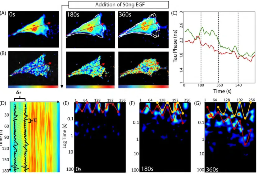
Fig. 1.2: Pair correlation analysis of a Rac1 FRET biosensor reveals Rac1 activity to be spatiotemporally regulated by a dynamic gradient of protein mobility.
10
Fig. 1.2: Pair correlation analysis of a Rac1 FRET biosensor reveals Rac1 activity to be spatiotemporally regulated by a dynamic gradient of protein mobility.
(A) Intensity image of a NIH3T3 cell expressing the Rac1 dual chain FRET biosensor in the donor channel before and after stimulation with epidermal growth factor (EGF). The white traces outline the cell’s position(s) from the previous panel(s). (B) Same cell as in (A) pseudo-colored according to donor lifetime. The blue to red color range corresponds to a change in lifetime from 2 to 3ns and therefore low to high Rac1 activity. The tau phase (in ns) is derived from phasor analysis of the fluorescence decay, as in [3]. Shorter tau-phase times correspond to higher FRET activity. (C) Average lifetime analysis of the first 10 pixels (back of the cell, green time series) and the last 10 pixels (front of the cell, red time series). This comparison reveals that after EGF stimulation Rac1 is activated earlier at the front than the back of the cell. (D) The intensity carpet that is derived from line scans acquired across the axis of the cell in (A). (E) Pair correlation analysis of the intensity carpet acquired before EGF stimulation. The highlighted data shows Rac1 molecular flow is uniform: it takes about 0.03s to traverse 0.8μm (pCF(8)). (F) Pair
correlation analysis of the intensity carpet acquired 180s after EGF stimulation. The highlighted shows Rac1 molecular flow is non-uniform. At the back of the cell, traversing 0.8μm takes about 0.03s; this time becomes gradually longer towards the front of the cell. The second set of highlighted data (yellow curve) is not significantly different from the first (red curve). (G) Pair correlation analysis of data acquired 360s after EGF stimulation. The mobility gradient is steeper (red curve); the delay time ranges from 0.05s at the back to 1.2s at the front. A second gradient emerges (yellow curve); the delay times range from 0.03s to 0.08s.
The simulation in Fig. 1.1 (Fig. 1.1H), wherein each barrier has equivalent affinity for Rac1, qualitatively matches the mobility of Rac1 in an unstimulated cell (Fig. 1.2E); that is, Rac1 mobility is uniform across the cell. However, in a stimulated cell, Rac1 shows variable mobility across the cell (Figs. 1.2F and 1.2G), possibly due to variable density of actin and hence variable Rac1 binding affinity. It may be that Rac1 interacts with different substrates with
varying affinities in the membrane, and therefore, Rac1 mobility depends on cell polarization in response to external cues. We next perform simulations guided by this hypothesis.
1.4
Gradient of Rac1 Molecular Flow Produced by Actin Island Simulations
11
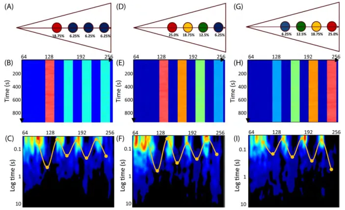
affinity for Rac1. Calculating the pCF carpet (Fig. 1.3C) reveals that Rac1 molecular flow is slowest in the island with highest affinity, slightly faster in the other three islands and fastest outside the islands. Hence the islands’ affinity inversely correlates with local Rac1 mobility.
Fig. 1.3: Simulations with islands of varying binding affinity.
(A) A simulation set-up showing the rear (leftmost) island binds on average 18.75% of all Rac1, and each of the other three bind 6.25% on average. Unbound Rac1 diffuses with D = 10μm2/s. If bound, Rac1
diffuses with D = 1μm2/s. (B) The resulting intensity carpet shows the highest accumulation at the rear
island. (C)The pCF carpet (yellow curve) reveals four arc features, which indicate regions of slow
12
Next, we extend our model by varying the affinity of each actin island. Specifically, islands closer to the leading edge have lower affinity than islands near the trailing edge (Fig. 1.3D). The intensity carpet shows four regions with different intensities (Fig. 1.3E). As before, the average intensity in each of the four regions is directly proportional to the binding affinity. The pCF carpet (Fig. 1.3F) shows a gradient of molecular flow; wherein, Rac1 mobility is faster towards the leading edge. We can reverse this gradient by reversing the island affinities (Fig. 1.3G). This model produces a pCF carpet (Fig. 1.3I) qualitatively similar to the one observed from in vivo data (Fig. 1.2F). That is, there is a diffusive gradient such that Rac1 mobility is slower towards the leading edge. Consistent throughout all our simulations, we find the characteristic time to diffuse around or through an actin island is proportional to the island’s binding affinity. We find that this mechanism to spatially regulate molecular flow is quite robust; the affinity of the actin island dictates the mobility at that location.
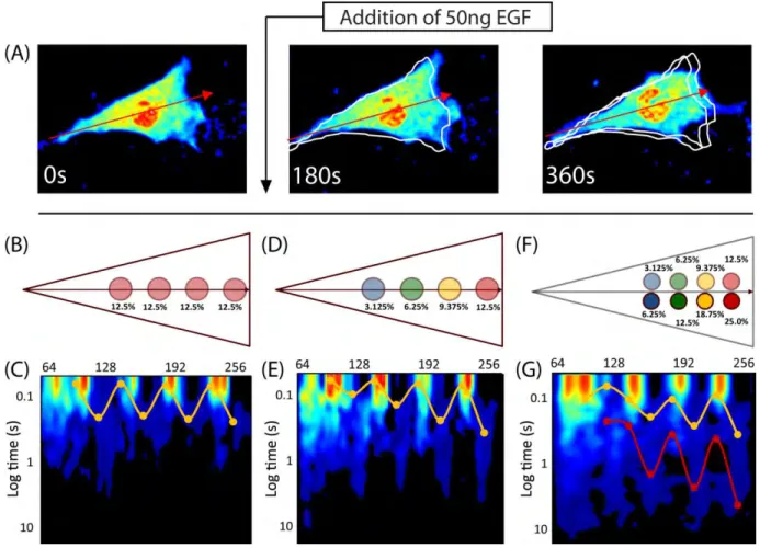
Finally, we aimed to reproduce the molecular flow observed 6 minutes after EGF
13
combining the intensity carpets, we perform pCF analysis. The resulting pCF carpet shows two gradients of molecular flow: one for each Rac1 population (Fig. 1.4G). Based on our previous results, we know the red curve corresponds to the high affinity active Rac1 population, and the yellow curve corresponds to the low affinity active Rac1 population. Our results indicate actin islands, which reversibly bind Rac1 and slow its diffusion, are sufficient to produce the spatially dependent molecular flow observed in vivo. Additionally, we find that if active and inactive Rac1 have different affinities for actin, then these two subpopulations would show different diffusive behaviors, similar to what has been observed experimentally.
Fig. 1.4: Investigating the cellular substructure during three stages of EGF stimulation by comparing pCF carpets.
14
front, which is less than the simulation in Fig 1.3G. This arrangement of islands is similar to what we expect is present in vivo. (E) pCF analysis reveals four arc features of differing lengths, co-localized with the actin islands. Rac1 mobility is slower towards the front of the cell. (F) Modeling two populations of Rac1 by the superposition of two actin island gradients: one with twice the affinity (Fig. 1.3G) as the other (Fig. 1.4D). We combine the intensity carpets of the two simulations and perform pCF analysis. Although the two sets of islands are superimposed, here, we separate them for illustrative purposes. (G) The resulting pCF carpet for a cell with two populations of Rac1. We find two distinct gradients as highlighted by the curves: one for each population. The red curve corresponds to the Rac1 population with the higher actin affinity.
1.5 Discussion
Here, we developed a computational platform for performing stochastic simulations of intracellular diffusion to study how actin islands are organized to spatially regulate the mobility of signaling molecules. Our simulation platform allows the location, shape, protein binding and unbinding rates and diffusion rate for each island to be varied independently. This flexible computational model allows us to probe what cellular architectures underlie key features of pCF carpets calculated from in vivo experiments using a Rac1 biosensor.
15
(Fig. 1.4C) experiments suggests actin islands are present before EGF stimulation (Figs. 1.4A – C). Next, to test our hypothesis that actin island affinity regulates molecular flow, we performed simulations with actin islands of varying affinity (Figs. 1.3G and 1.4D) and compared these with the in vivo observed mobility gradient (Fig. 1.2F). The pCF carpets from these simulations (Figs. 1.3I and 1.4E) show a mobility gradient similar to the one observed in vivo (Fig. 1.2F); wherein, the time it takes for Rac1 molecules to flow 0.5μm is based on their proximity to the leading edge. Hence, the observed mobility gradient from the in vivo experiment is consistent with the presence of actin islands with progressively stronger affinity for Rac1 in moving from the rear to the front of the cell. Finally, we aimed to reproduce the in vivo observed dual regulation of Rac1 indicated by two distinct mobility gradients (Fig. 1.2G). We combine the results of two
simulations, which are identical in every aspect, except for the actin islands’ affinities (Fig. 1.4F). The resulting pCF carpet (Fig. 1.4G) shows two sets of arc features, similar to the ones observed in vivo (Fig. 1.2G). Hence, the two sets of mobility gradients observed from the in vivo experiments (Fig. 1.2G) may indicate the presence of two forms of Rac1 (e.g. inactive and active) with different affinities to the actin islands.
16
partner may account for the discrepancy in conformation sampling. We discuss the implications of each possible technique for controlling the affinity of actin islands below.
Based on the results of our experimental and computational investigations, we propose that cells can spatially regulate the molecular flow of certain proteins through the use of actin islands. In particular, our results suggest that cells can position the islands in regions where slower flow is desired, e.g. to sequester Rac1 at the leading edge. Because an island regulates molecular flow only locally, the cell can utilize actin islands only where needed. Additionally, the extent to which Rac1 mobility is slowed can be regulated by adjusting the binding affinity. Actin is known to reorganize in seconds [9], and this reorganization may play a role in regulating the position, size, shape and concentration of the islands. In turn, the concentration of actin in each island could affect the affinity for Rac1: denser islands have higher affinity than less dense islands. Organizing actin islands allows cells to spatially regulate molecular flow and therefore establish internal concentration gradients.
17
(possibly the inactive and active forms) with different affinities for the actin islands and subsequently separately regulated flow.
1.6 Methods
We developed a simulation platform to test our proposed model of Rac1 behavior. Our program returns intensity carpets that are directly comparable to experimentally measured intensity carpets. As with the in vivo experimental data, we perform pair correlation analysis on the in silico intensity carpets to determine any spatial dependence on the diffusion constant. Our goal was to determine sufficient conditions for recapitulating the spatial dependence on the diffusion constant observed in vivo, by rearranging and varying the binding constant of the actin islands. Our program uses a particle-based stochastic simulation algorithm to simulate reactions and diffusion. Individual Rac1 molecules are modeled as point particles in continuous space and capable of reacting and diffusing discretely in time. This algorithm allows us to closely mimic the stochastic diffusion of Rac1 molecules inside the cell. A computational model that captures these natural fluctuations in concentration is imperative for pair correlation analysis.
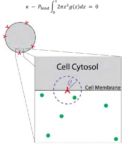
1.6.1 Simulation Algorithm
A cell migrating on a 2D substrate in the xy-plane is modeled as an isosceles triangle whose base represents the direction of migration (Fig. 1.5). In this system, diffusion along the z-axis is largely inconsequential, because the molecular counts used to produce the intensity
18
Fig. 1.5: Simulation Geometry.
The cell boundary is shown in green as an isosceles triangle 25.6µm wide and 5µm tall. The actin islands are shown as black circles with 1µm radii. As discussed in the text, unbound Rac1 molecules are free to diffuse throughout the cell and reflect off the cell boundary. Bound Rac1 molecules diffuse slower and are restricted to the inside of the island in which they are bound. We can individually set the KD of each island
thereby setting, on average, the percent of the total Rac1 population bound to each island. The 256 magenta boxes represent the (0.1μm)2 bins used
to generate the intensity carpet; these bins do not affect the behavior of the molecules.
20
As suggested by [10], we use the Euler-Maruyama method [11] to perform stochastic simulations of diffusing particles. That is, knowing the current position of a Rac1 molecule, (x(t), y(t)), we calculate its position at the next time step, (x(t+Δt),y(t+Δt)), using the following
equations:
( ) ( ) √ (1.1a)
( ) ( ) √ (1.1b)
Here, D is the diffusion constant, Δt is the time step and the Wn’s are random numbers drawn
from a Gaussian distribution with a mean of 0 and a variance of 1. Unbound Rac1 molecules diffuse freely inside the cell with Dunbound = 10μm2/s. The boundaries of the cell are reflective.
Hence, if a molecule attempts to leave the cell (i.e. the diffusion calculation places the particle outside the cell boundaries), then the molecule is elastically reflected back inside the cell. Bound Rac1 molecules diffuse freely inside the actin island to which they are bound with Dbound =
1μm2/s. The boundary of the island is reflective only to bound molecules. Hence, if a bound
molecule attempts to leave the island (i.e. the diffusion calculation places the particle outside the island), then the molecule is elastically reflected back inside the island. Consequently, all bound Rac1 molecules are restricted to an island. The converse, however, is not true; not every Rac1 molecule positioned inside an actin island is bound. Unbound Rac1 molecules, which are
positioned inside an island, are considered to be diffusing over/under/through that island without penalty. It is only in this condition that a binding reaction may occur.
21 ( ) (
) (1.2)
Here, kon is the rate constant for binding to the island; Δt is the time step; v is the volume of the
island, and V is the volume of the entire cell (we assume the cell is 1µm thick).
Separately, we calculate all unbinding events between time steps. If a Rac1 molecule is bound at time t, then its state can switch to unbound with probability Punbind:
(1.3) Here, koff is the dissociation rate constant. When changing the state of a Rac1 molecule, due to
either a binding or unbinding reaction, we do not change the position of the molecule.
We calculate the reaction rates based on an average fraction of total Rac1 molecules that we wish to have bound in each island:
(1.4)
Here, f is the average fraction of Rac1 molecules bound in the island, and 1–F is the average fraction of Rac1 molecules not bound in any island. Note kon should be expressed in units of
μm3/s using a conversion factor such as 0.6022/(nM·μm3). Additionally, the fraction of
molecules bound at each island also relates to the reaction probabilities:
(1.5)
For example, if we desire each of the four islands to bind, on average, 6.25% of all Rac1 molecules, then F = 0.25 and for each island f = 0.0625. We know the volumes (v and V) from Fig. 1.5. Unfortunately, instead of a value for Pbind or Punbind, we are only left with a ratio between
22
We choose the off-rate such that the time-scale for unbinding is equal to the time-scale for a bound molecule to diffuse the length of the island:
√
( )
( ) (1.6)
This rate is substituted into Eq 1.3 to get Punbind, which in turn, is substituted into Eq 1.5 to get
Pbind. In this case, Punbind = 0.5×10⁻⁶ and Pbind = 0.85×10⁻⁶ for a time-step Δt = 1μs. The reaction
probabilities for each simulation are annotated in the Supplemental Methods (Section 1.7.5). 1.6.2 Pair Correlation Carpet
A line-scan technique was used during in vivo experiments [3,5,6], which reports the fluorescence intensity of Rac1-GFP molecules. The intensity is sequentially measured from pixel 1 to, about, pixel 300 to complete one line scan. Many line scans are taken and these scans are compiled into an intensity carpet on which pair correlation analysis can be performed. To produce an in silico analog to the intensity carpet, we tally the particles by their position as they are simulated (see above). To establish the line along which we will scan, we arrange 256 square bins sized (0.1μm)2 along the center of the cell (Fig. 1.5). We cumulatively count the number of
Rac1 molecules positioned inside a bin during a 25µs time window. Each bin is scanned sequentially; that is, we tally the counts from the first bin for the first 25µs; then we tally the counts from the second bin for the second 25µs etc. After 6.4ms (256*25μs) one full line scan is complete, and the next line scan begins immediately. Each intensity carpet has 47000 lines, corresponding to a simulation time of just over 5min. The bin size (0.1μm)2 is roughly equivalent
23
To better understand the flow of particles within the cell, we calculate the pair correlation function (pCF) from the intensity carpet. First, we extract the intensity time trace (intensity versus time) for each pixel (e.g. cartooned white curves in Fig. 1.1D). Second, we calculate the correlation coefficient between two of these traces while sweeping two parameters in space (δr) and time (τ). With regards to space, we consider the traces of two pixels a distance δr apart; note that when δr = 0, we are computing the autocorrelation value (Figs. 1.1E and 1.1F). With regards to time, we shift the trace from the second pixel by τ seconds. Hence the correlation coefficient for a pixel given a pair of parameters (δr, τ) describes the likelihood a particle will diffuse from that pixel to a pixel δr away in τ time. A value of 0 indicates this diffusive trajectory is
impossible; while, a value of 1 implies a complete directed flow. Note that there is directionality in our pCF. A left to right calculation (e.g. correlating pixel 0 with pixel 5) describes the
diffusion landscape from the back of the cell to the front (line scans are taken as such). A right to left calculation (e.g. correlating pixel 5 with pixel 0) describes the diffusion landscape from the front of the cell to the back.
24
1.7 Supplemental Methods
1.7.1 Analyzing pCF Carpets
Fig. 1.6: Gaussian analysis of pair correlation carpets to extract average delay time(s) Rac1 takes to diffuse along simulated and in vivo line scans.
25 1.7.2 Simulation Program Details
We simulate 100,000 molecules, which, given the dimension of the cell (Fig. 1.5) and an assumed height of 1µm, corresponds to a concentration of 0.94µM. We monitor each molecule’s position: (x,y) and state: ‘bound’ or ‘unbound’. All molecules are updated simultaneously during each time step. Depending on the state of the particle, we calculate its new position (Diffusion) then determine if its state changes (Reaction). Consider the following, short pseudo-code.
For each time step:
I. ‘Unbound’ molecules: diffuse with Dunbound = 10 µm2/s
a. If outside the cell, then reflect position back inside cell
b. If inside an island, then generate a random number to determine if ‘bound’ II. ‘Bound’ molecules: diffuse with Dbound = 1 µm2/s
a. If outside the island, then reflection position back inside the island
b. Generate random number to determine if ‘unbound’
1.7.3 Calculating Diffusion Steps
We use Eq 1.1 to calculate the molecules’ new position. That is, for each spatial dimension: ( ) ( ) √ . Here, W is a random number drawn from a Gaussian
Distribution with mean 0 and variance 1. We calculate this random number using the Box-Muller Method, as implemented in the “curand” library of the CUDA 4.0 Toolkit.
Molecules are restricted to certain regions: ‘unbound’ molecules must remain inside the cell, and ‘bound’ molecules must remain inside the island to which they are bound. These rules are enforced by imposing reflective boundaries at the cell wall and the edges of the actin islands respectively. In the next two sections, we discuss how the reflections for each boundary are calculated.
Reflections off Cell Boundaries
26
boundary traversing from (25.6, –2.5) to (25.6, 2.5) (Fig. 1.5). We describe each line in the form: ax + by + c = 0 (restricting a > 0). Specifically, the ‘top’ boundary is:
(1.7)
The ‘bottom’ boundary is:
(1.8)
The ‘right’ boundary is:
(1.9)
Let (x', y') be the position that lies outside the cell. Accordingly, the distance from the point (x', y') to a line can be calculated using the expression:
| |
√ (1.10)
Hence, the point (x', y') can be reflected off the ‘top’ and ‘bottom’ boundaries using the equation:
[ ] [ ]
√ [ ] (1.11)
To reflect the point (x', y') off the ‘right’ boundary, we calculate:
| | (1.12)
During the diffusion of an ‘unbound’ particle, we check if the new position is outside the cell. That is, the position is above the ‘upper’ boundary: ( ) , below the ‘lower’
27
cases that lead to an infinite check/reflect loop. These rare cases occur when the position is close (within numerical error) to a corner of the cell boundary. These cases are resolved during
diffusion in the next time step.
Reflections off Actin Island Boundaries
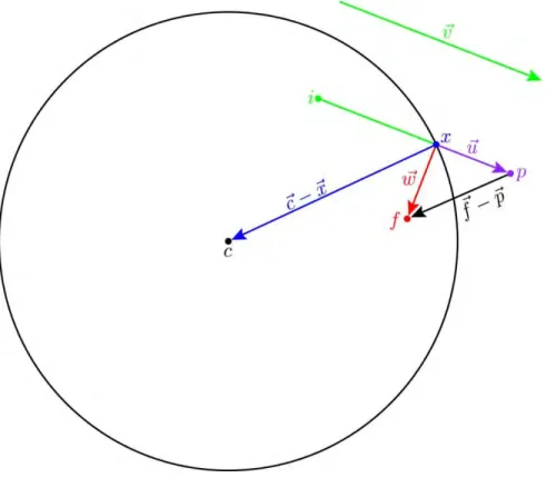
To reflect a particle inside an actin island (which is a circle in our 2D model), we must know the particle’s initial position inside the island, ⃑, the proposed position outside the island, ⃑, and the center position of the island, ⃑ (Fig. 1.7).
Fig. 1.7: Important Vectors for Reflecting Inside Actin Island.
Here, we diagram an example of a ‘bound’ particle being reflected back inside an actin island while diffusing during a single time step. Initially the particle is at point i; after freely diffusing for one time step, the proposed final position is at point p. The particle crosses the circular actin island’s boundary at point x. For a reflective boundary, the true final position is at point f. Important vectors between these points are indicated. See the text below for details on how to determine the final, reflected position given the points i, p, c and the radius r of the island.
28
⃑ ⃑ ⃑ (1.13)
Because ⃑ lies on the boundary, we know the following constraint: ( ⃑ ⃑) ( ⃑ ⃑) , where is the radius of the island. After substituting Eq 1.13 into the constraint, we solve for tx:
⃑ ( ⃑ ⃑) √ ‖ ⃑‖
( ⃑ ( ⃑ ⃑)) (‖ ⃑‖ )( ‖ ⃑ ⃑‖ )
(1.14)
Hence, numerically, ⃑ is found by substituting known values into Eq 1.14 then Eq 1.13.
The vector ⃑⃑ ( ⃑⃑ ⃑ ⃑) is the erroneous portion of the particle’s trajectory; that is, the portion in which the particle traveled outside the actin island. To correct the trajectory and reflect the particle back inside the island, we reverse the radial component of ⃑⃑. The vector ⃑⃑⃑ is the corrected continuation of the trajectory. The magnitudes of ⃑⃑ and ⃑⃑⃑ are equivalent. They differ by twice the radial component of ⃑⃑ (Eq 1.15). We denote the direction pointing towards the center of the island as ( ⃑ ⃑)̂ ‖ ⃑ ⃑‖ ⃑ ⃑ ⃑ ⃑.
⃑⃑⃑ ⃑⃑ ( ( ⃑⃑ ( ⃑ ⃑)̂ ) )( ⃑ ⃑)̂
⃑⃑⃑ ⃑⃑ ( ) ( ⃑⃑ ( ⃑ ⃑))( ⃑ ⃑)
(1.15)
And, because ⃑⃑⃑ ⃑⃑ ⃑ ⃑, we can calculate ⃑ from Eq 1.15 using the expression:
29
this re-check will fail; that is, even after reflecting the particle, the new position will still be on the edge of or outside the island. For those scenarios, we repeat the entire process and calculate a different diffusion step. We find these pathological cases occur when the starting position is close (within the numerical error) to the island boundary.
1.7.4 Calculating Reaction Probabilities
After calculating the diffusion step, an ‘unbound’ molecule positioned in an island has a probability to bind, and a ‘bound’ molecule has a probability to unbind. We calculate these probabilities such that the reactions are simulated in a biophysically relevant regime. Our
proposed model for the diffusion of Rac1 in the cell does not (nor is it necessary to) speculate on exact values of the reaction rates for the different actin islands. Instead, our model proposes different binding affinities in each island. Below, we derive the relationship between the reaction rates of each island and the probabilities of reaction.
We write out the Master Equation for the binding reaction on the ith island: let A denote
the number of ‘unbound’ Rac1 throughout the cell and denote the number of ‘bound’ Rac1 in the ith island.
̇ ( ) ( ) (1.17)
Here, and are the reaction rates for the ith island, and V is the volume of the cell (we set the cell thickness to 1µm). The unbinding term, ( ) , describes the number of molecules which will unbind from the ith island during the infinitesimal time dt. The unbinding term is
30
during the infinitesimal time dt. The binding term is derived from multiplying the on-rate by the “concentration” of the island and by the number of molecules eligible to bind to the island.
( ) ( ) ( ) ( ) (1.18)
Here, vi is the volume of the ith island; hence, is the “concentration” (since the unit for
concentration is inverse volume) of actin. The number of molecules eligible to bind is the
number of unbound molecules located inside the island; this value is equal to the total number of unbound molecules, A, scaled by the probability of being located in the ith island: .
At equilibrium, the number of binding and unbinding events is balanced; we set Eq 1.17 equal to 0 and solve for the KD.
(1.19)
We multiply the right-hand-side by
, in order to rewrite the equation in terms of the fraction
(with respect to the entire population) of bound and unbound molecules. We denote the fraction of molecules bound to the ith island as
. We write the fraction of unbound molecules as
∑ , where is the total fraction of molecules bound in all islands.
(1.20)
We determine the probability a molecule reacts (both binding and unbinding processes) in a time Δt. We choose a sufficiently small time step (1µs) such that we may assume a single molecule can perform only one reaction (bind or unbind) during that time step. Hence, we may separately solve the differential equations describing each reaction (i.e. each term in Eq 1.17).
31
( ) ( ) ( )
(1.21)
Where ( ) is the number of molecules bound to the ith island as a function of time. We choose
a small time step such that only the ith island unbinds.
̇
( )
(1.22)
Substituting Eq 1.22 into Eq 1.21, we find:
(1.23) The probability any unbound molecule binds to the ith island during a time step is equal
to:
( ) ( ) ( )
(1.24)
Where A(t) is the number of unbound molecules as a function of time. We choose a small time step such that only the ith island binds.
̇
( )
(1.25)
Substituting Eq 1.25 into Eq 1.24, we find:
32
Eq 1.26 describes the probability that any unbound molecule will bind to the ith island. We
rewrite this overall probability as joint probability of, one, the probability an unbound molecule is located inside the ith island and, two, the probability that the same molecule binds:
( ) (1.27) Hence, the probability that an unbound molecule located inside an actin island binds during a time step Δt is given by:
( ) ( ) (1.28) The exponentials in Eqs 1.23 and 1.28 can be simplified by using the first two terms of their Taylor Expansion. These two expressions for the probability of unbinding and binding can then be written as:
(1.29)
(1.30)
We combine Eqs 1.20, 1.29 and 1.30 to get three equal expressions for the KD relating the
reaction rates, fraction bound in each island and the probabilities of reacting.
(1.31)
In every simulation, we customize the affinities for each island; that is, we choose the set of fi.
33
across an actin island in the ‘bound’ state (Eq 1.6). Table 1.1 summarizes the reaction rates, fraction bound and reaction probabilities for each simulation.
1.7.5 Full Set of Simulation Parameters
In all simulations, the volume of the cell (V = 64µm3), the volumes of all islands (v =
Simulation
Set-up ⃑ ⃑⃑⃑⃑⃑⃑⃑ ( ) ⃑⃑⃑⃑⃑⃑ ( ) ⃑⃑⃑⃑⃑⃑⃑⃑⃑⃑⃑⃑⃑⃑⃑ ⃑⃑⃑⃑⃑⃑⃑⃑⃑⃑
Fig 1.1C & 1.4B {0.125, 0.125, 0.125, 0.125} {0.5, 0.5 0.5, 0.5} {4.8, 4.8, 4.8, 4.8} {0.5×100.5×10-6-6, 0.5×10, 0.5×10⁻⁶-6} , {2.55×10
-6, 2.55×10⁻⁶,
2.55×10⁻⁶, 2.55×10⁻⁶} Fig 1.3A {0.1875, 0.0625, 0.0625, 0.0625} {0.5, 0.5 0.5, 0.5} 1.927, 1.927} {5.78, 1.927, {0.5×100.5×10-6-6, 0.5×10, 0.5×10⁻⁶-6} , {3.056×10
-6, 1.019×10⁻⁶,
1.019×10⁻⁶, 1.019×10⁻⁶}
Fig 1.3D 0.125, 0.0625} {0.25, 0.1875, {0.5, 0.5 0.5, 0.5} 6.5, 3.36} {13, 9.7, {0.5×100.5×10-6-6, 0.5×10, 0.5×10⁻⁶-6} , {6.79×10
-6, 5.09×10⁻⁶,
3.4×10⁻⁶, 1.7×10⁻⁶}
Fig 1.3G {0.0625, 0.125, 0.1875, 0.25} {0.5, 0.5 0.5, 0.5} {3.36, 6.5, 9.7, 13} {0.5×100.5×10-6-6, 0.5×10, 0.5×10⁻⁶-6} , {1.7×10
-6, 3.4×10⁻⁶,
5.09×10⁻⁶, 6.79×10⁻⁶}
Fig 1.4D {0.03125, 0.0625, 0.09375, 0.125} {0.5, 0.5 0.5, 0.5} {0.912, 1.75, 2.6, 3.5} {0.5×100.5×10-6-6, 0.5×10, 0.5×10⁻⁶-6} , {4.63×10
-7, 9.26×10⁻⁷,
1.39×10⁻⁶, 1.85×10⁻⁶}
Table 1.1 Reaction Rates and Probabilities
The reaction rates and corresponding probabilities are shown for each simulation presented in this chapter. Column 1 indicates a figure, which shows a cartoon sketch of a simulation. Column 2 shows the average fraction of molecules bound to each island. Columns 3 and 4 indicate the reaction rates for each island, and columns 5 and 6 show the corresponding reaction probabilities.
35 1.7.6 Generating an Intensity Carpet
To generate an intensity carpet as done in vivo [3,5,6] for our in silico data, we tally the number of molecules in each bin sequentially, measuring for 25µs at a time. If we label the 256 bins from 0 to 255 and let t be the current simulation time (in µs), then the current bin being tallied is
( ( )) (1.32)
Where ‘floor(x)’ is a function which returns the largest integer that is less than or equal to x. And where ‘mod’ indicates the modulo arithmetic operator. The tally is incremented for every particle positioned inside the current bin after diffusing and reacting. For example: for t ϵ [0, 24], we tally the particles in bin 0; for t ϵ [25, 49], we tally the particles in bin 1; for t ϵ [6375, 6399], we tally the particles in bin 255, and for t ϵ [6400, 6424], we tally the particles in bin 0. We store these tallies as a matrix with 256 columns (one for each bin), and 47000 rows (one for each line scan).
1.7.7 Hardware Details
This program was written in CUDA C using the CUDA 4.0 Toolkit. CUDA is a publicly available parallel programming architecture built for Generally Programmable Graphics
Processing Units (GPGPUs), specifically, those manufactured by the NVIDIA ® Corporation. Utilizing GPGPUs, we are able to simultaneously access hundreds of computational processors in parallel. Because each particle is independent of all others, we parallelize our algorithm at the particle level. That is, we launch one computational thread in the GPU for each particle in our simulation. Each thread performs all necessary calculations for reacting and diffusing a single particle. All threads and particles are periodically synchronized in time. Every 12.8ms of
36
37
REFERENCES
1. Burridge K, Wennerberg K (2004) Rho and Rac Take Center Stage. Cell 116: 167–179. 2. Machacek M, Hodgson L, Welch C, Elliott H, Pertz O, et al. (2009) Coordination of Rho
GTPase activities during cell protrusion. Nature 461: 99–103.
3. Hinde E, Digman M a, Hahn KM, Gratton E (2013) Millisecond spatiotemporal dynamics of FRET biosensors by the pair correlation function and the phasor approach to FLIM. Proc Natl Acad Sci U S A 110: 135–140.
4. Katsuki T, Joshi R, Ailani D, Hiromi Y (2011) Compartmentalization within neurites: its mechanisms and implications. Dev Neurobiol 71: 458–473.
5. Digman M a, Gratton E (2009) Imaging barriers to diffusion by pair correlation functions. Biophys J 97: 665–673.
6. Hinde E, Cardarelli F (2011) Measuring the flow of molecules in cells. Biophys Rev 3: 119–129.
7. Hinde E, Cardarelli F, Digman MA, Gratton E (2010) In vivo pair correlation analysis of EGFP intranuclear diffusion reveals DNA-dependent molecular flow. Proc Natl Acad Sci U S A 107: 16560–16565.
8. Moissoglu K, Slepchenko BM, Meller N, Horwitz AF, Schwartz MA (2006) In vivo dynamics of Rac-membrane interactions. Mol Biol Cell 17: 2770–2779.
9. Andrews NL, Lidke KA, Pfeiffer JR, Burns AR, Wilson BS, et al. (2008) Actin restricts FcepsilonRI diffusion and facilitates antigen-induced receptor immobilization. Nat Cell Biol 10: 955–963.
10. Erban R, Chapman SJ (2009) Stochastic modelling of reaction-diffusion processes: algorithms for bimolecular reactions. Phys Biol 6: 046001.
38
CHAPTER 2: A MODEL OF GRADIENT SENSING IN THE CONTEXT OF YEAST MATING2
Introduction
Sensing an external chemical gradient is a fundamental process in cell biology present in areas such as cancer metastasis, wound healing and embryogenesis. This ability, of decoding spatial information, allows cells to move or grow towards a favorable environment or away from an unfavorable environment. Most eukaryotic cells use a spatial detection mechanism, wherein one portion of the cell membrane has more active receptors than the other regions. This skewed distribution of active receptors reflects the external chemical gradient. Some cells, like yeast (S. Cerevisiae), are capable of detecting extremely shallow gradients, wherein the noise from
molecular diffusion and stochastic reactions is thought to obscure the desired spatial information. Accordingly, various mechanisms have been proposed to explain how yeast cells overcome this poor signal to noise ratio. To quantitatively assess these mechanisms, we develop a particle-based stochastic reaction-diffusion model. This approach monitors the position of individual molecules and models the two sources of noise present during gradient sensing: diffusion and stochastic binding and unbinding reactions. Here, we first outline the model used to investigate the distribution of active receptors by simulating the reversible binding reaction between pheromone and receptor. Second, to evaluate two potential noise-reduction mechanisms, we discuss adding receptor endocytosis and the pheromone protease Bar1 to our model.
2 This chapter is being drafted as part of a publication to be submitted to the journal PLoS Computational Biology. It
39
2.1 Overview
We first describe the important biophysical features of gradient sensing that the model should capture. The model must be able to resolve individual signaling molecules in a
continuous 3-dimensional space. It also should faithfully capture the stochastic properties of diffusion of both the extracellular signaling molecules and receptors in the cell membrane, and of the biochemical reactions involved in ligand binding and release and receptor internalization. For these reasons, we choose a Particle-Based Stochastic Reaction-Diffusion model. When
simulating this model, molecules are modeled as non-colliding point particles which can stochastically diffuse and react, discretely in time and continuously in space.
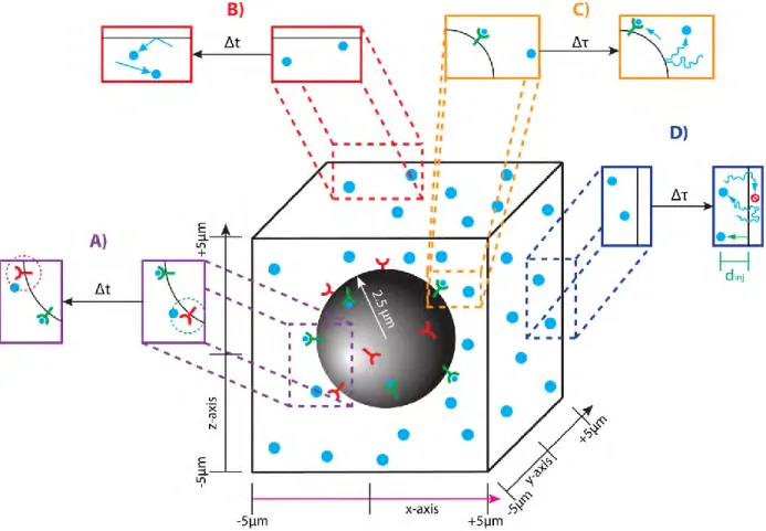
We simulate molecules in a cubic volume (10μm by 10μm by 10μm). We model the cell as a sphere with a radius of 2.5μm at the center of the volume (Fig. 2.1). The state of the system is defined by the position of every pheromone and receptor molecule as well as the state of each receptor (occupied or empty). Pheromone molecules cannot be located inside the cell, and receptor molecules are restricted to the surface of the cell. Given the current state at time t0, we
determine the subsequent state at time t0 + Δt, where Δt is a time step of fixed length, by
calculating all binding reactions, unbinding reactions and diffusion of each molecule. A binding event occurs during the time step, Δt, with probability Pbind (Table 2.1), if a pheromone molecule
is within rbind = 4nm (binding radius) of an unbound receptor (Fig. 2.1A). An unbinding event
occurs during the time step, Δt, with probability Punbind = 1.1×10⁻⁹ (Table 2.1). A bound receptor
40
binding radius (4nm). Our model captures the stochasticity due to reactions and diffusion, and our model monitors the exact position of all molecules in a 3D space. Below, we explain the microscopic rules that each molecule follows.
Fig. 2.1: Simulations on our Particle-Based Stochastic Reaction-Diffusion Model
41 Table 2.1: A Typical Parameter Set
The first portion contains all the parameters necessary to uniquely define a simulation of our model. The second portion contains additional, informative values that are calculable from the first portion.
Parameter Value Description
Customizable Parameters
XDom 10 µm Length of x-domain
YDom 10 µm Length of y-domain
ZDom 10 µm Length of z-domain
Δt 1 µs Time Step
Δτ 50 µs Coarse Time Step
R 2.5 µm Radius of Cell
Dα 125 µm2/s Pheromone Diffusion Constant [1]
Grad 0.1 nM/µm Pheromone Concentration Gradient along x-axis
Conc 6.9 nM Background Pheromone Concentration (equal to K
D)
DSte2 0.0025 µm2/s Receptor Diffusion Constant [2]
N 10000 Number of Receptors on Cell Surface [3–6]
kon 1.6×10⁵ (M·s)-1 Binding Rate [7]
koff 0.0011 s-1 Unbinding Rate [7]
rbind 4 nm Binding Radius
runbind 4 nm Unbinding Radius
Additional Values
Pbind 0.002 Binding Probability
Punbind 1.1×10⁻⁹ Unbinding Probability
KD 6.9 nM Pheromone/Receptor Dissociation Constant [7]
chigh 7.4 nM Concentration at High Boundary (x = 5µm)
clow 6.4 nM Concentration at Low Boundary (x = –5µm)
ninj High 19.88 Average Number of Pheromone to create at High Boundary
ninj Low 17.19 Average Number of Pheromone to create at Low Boundary
dinj Random from Eq 2.6 List of injection distances: random numbers from Eq 2.6
2.2 Binding Reactions
42
binding radius is calculated from the binding rate and the diffusion constants of the two molecular species:
(
) (2.1)
This expression can be derived from Fick’s Law of diffusion and works well when the reaction is diffusion limited; however, α-factor binding to Ste2 is not diffusion limited. Using the rates reported in the literature, this approach requires a binding radius on the order of Angstroms, which is much smaller than the size of Ste2 (GPCRs protrude about 4nm outside the cell
membrane [8]).As discussed by Erban and Chapman the unrealistic binding radius results from the assumption that the binding probability is 100% [9]. That is, a ligand molecule within the binding radius of an unbound receptor binds with certainty. The model put forward by Erban and Chapman, removes this assumption and establishes a mathematical framework, in which the binding probability is a function of the binding radius [9,10]. That is, a ligand molecule within a specified binding radius binds with a probability that produces an average binding rate consistent with the macroscopic rate constant kon. We choose the binding radius to be 4nm and calculate the
binding probability by numerically solving the system:
∫ ( ) (2.2)
where,
( ̂) ( ) ∫ ( ̂ ̂ ) ( ̂) ̂
∫ ( ̂ ̂ ) ( ̂ ) ̂
43 ( )
√ ( [
( )
] [
( )
])
√ ( )
derived by Erban and Chapman [10]. For example, using the values for Δt, kon, Dα, DSte2, rbind and
runbind shown in Table 2.1, a pheromone molecule has a 0.2% chance of binding. We provide a
detailed description of how we calculate the probability in Section 2.9. Our customized binding radius and binding probability make our method more accurate and physically realistic than other methods.
2.3 Unbinding Reactions
A ‘bound’ receptor molecule unbinds its ligand molecule in the following way. A new ligand molecule is created a fixed distance away from and in a random direction from the
receptor (Fig. 2.1A). The fixed distance is called the unbinding radius (runbind). We avoid creating
the newly released pheromone molecule inside the cell. Lastly, the receptor molecule is switched to the ‘unbound’ state. Given an experimentally measured unbinding rate, we can calculate the unbinding probability, that is, the probability each ‘bound’ receptor has to unbind, using:
[ ] (2.3) As with the binding radius, we also set the unbinding radius to be 4nm.
2.4 Diffusion of Pheromone
44
( ) ( ) √ (2.4a)
( ) ( ) √ (2.4b)
( ) ( ) √ (2.4c)
The factors W1, W2 and W3 are each random numbers drawn from a Gaussian Distribution with a
mean of 0 and a variance of 1. The new position is modified if it is located outside the simulation volume or inside the cell. Reflecting boundary conditions are imposed at four of the boundaries: y = ±5μm and z = ±5μm. Any pheromone molecule that diffuses outside of these boundaries (y < –5μm, or y > 5μm, or z < –5μm, or z > 5μm) is reflected back into the volume (Fig. 2.1B). Additionally, pheromone molecules reflect off the surface of the cell, because the cell membrane is impermeable to pheromone (Fig. 2.1C). This boundary condition prevents pheromone
molecules from being located inside the cell. Details for calculating the reflection off the cell surface are provided in Section 2.10.
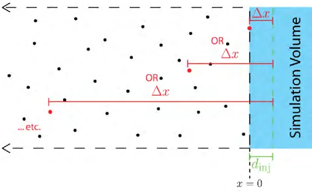
The last two boundaries, x = ±5μm, are each uniquely defined, because we wish to establish a linear pheromone gradient along the x-axis. We describe two different methods for treating the x = ±5μm boundaries, each of which can establish a gradient. In method 1, each boundary has a fixed concentration. In method 2, one boundary has a fixed concentration while the other is partially absorbing. The next two sections describe the physical interpretation and algorithmic implementation for each method.
2.4.1 Pheromone Gradient – Method 1
45
are added to and removed from the simulation volume in processes called ‘injection’ and ‘ejection’, respectfully (Fig. 2.1D).
For ejection, we remove all pheromone molecules located outside the boundaries (x < – 5μm, or x > 5μm) (Fig. 2.1D). For injection, we create a number of new pheromone molecules and position them near either the x = 5μm or x = –5μm boundary. On average, the number to inject at each time step is calculated using the equation:
√
(2.5)
where c is the desired pheromone concentration at the boundary; a is the area of the boundary (100μm2 for most of our simulations); D
α is the diffusion constant for pheromone molecules, and
Δτ is the elapsed time between two injection processes. The derivation of Eq 2.5 is found in Section 2.11. Although Eq 2.5 provides the average number of molecules to be injected, due to the stochastic nature of diffusion, the actual number injected can vary for a given time step. During an injection step, the number to inject is a random number drawn from a Poisson distribution with a mean of ninj. The position of a newly injected molecule is also determined
randomly. The ‘y’ and ‘z’ positions are determined from a uniform probability distribution across their respective domains (e.g between –5μm and 5μm, inclusively). The ‘x’ position is calculated as a random distance, called the ‘injection distance’, into the simulation volume from the boundary (Fig. 2.1D). The probability distribution function for the injection distance, dinj, is
given by:
( ) [ erf(
√ )] (2.6)
46
given by Eq 2.6, we select a random value from a pre-calculated long list. This list has more than 12 million random values whose distribution matches Eq 2.6.
For computational efficiency, injection and ejection of particles are implemented on a slightly coarser time scale, Δτ, than the time scale for diffusion Δt. It is important to note that ejection and injection must be calculated on the same time scale. Details and justification for the two time scales are discussed below in Section 2.6: “Algorithm Overview”.
2.4.2 Pheromone Gradient – Method 2
In this method, we model a fixed concentration at one boundary (x = 5μm), while the other boundary (x = –5μm) is partially absorbing. We use this method for simulations in which pheromone molecules flow toward the cell from one direction ( ̂) (Section 3.5).
At the x = 5μm boundary, ejection is the same as method 1. The average number of molecules to inject, ninj, at each time step is given by:
( √
) (2.7)
The derivation of Eq 2.7 is found in Section 2.11. Note that in addition to defining the desired concentration at the boundary, c, we also define the desired gradient at the boundary: g. Eq 2.5 is a special case of Eq 2.7, in which there is no gradient (g = 0 nM/μm) outside our volume (x > 5μm).