International Journal of Communication Networks and Information Security (IJCNIS) Vol. 11, No. 1, April 2019
SEPCS: Prolonging Stability Period of Wireless
Sensor Networks using Compressive Sensing
Dina Omar
1and Ahmed M. Khedr
22Computer Science Department, University of Sharjah, Sharjah 27272, UAE 1,2Mathematics Department, Zagazig University, Zagazig, Egypt
Abstract: Compressive sensing (CS) is a developed theory that is based on the fact that a small number of linear projections of a sparse data contain enough information for reconstruction. In this paper, we propose a routing protocol called SEPCS for clustered Wireless Sensor Networks (WSNs) using CS. SEPCS combines a new clustering strategy with CS theory for prolonging stability period and network lifetime in WSNs. The simulation results demonstrate that SEPCS effectively prolong the stability period and the lifetime of the network compared to existing protocols.
Keywords: Cluster-based, Compressive sensing, Stability period, Network lifetime, Wireless sensor networks.
1.
Introduction
The wide development in wireless communications have specifically given us the capability to produce small, low-cost sensor nodes that can wirelessly reach each other and compose a WSN. WSNs are made of a huge number of sensors deployed in a certain area. The sensors would transform physical data into a form that would make it easier for the user to understand. WSN technology is increasing quickly and becoming easier and cheaper to afford, granting different types of applications such as monitoring (seismic, health environments, etc.), control (tracking, object detection etc.), and surveillance (battlefield surveillance), topology and perimeter detection [1-6, 23-24]. WSNs are distinguished by higher unreliability, low power, computation and memory constraints and denser deployment of sensors. Therefore, the unique constraints and properties produce many challenges for the development and application of WSNs. Sensors are battery-powered and are expected to operate without attendance for a relatively long period of time. It is very difficult to recharge or replace batteries for the sensors. Due to the difference of WSNs from other wireless networks such as ad hoc networks, routing in WSNs is not easy task. All applications of WSNs have the requirement of transmitting the sensed data from multiple sensors to a specific destination called sink or Base Station. For this reason, resource management is required in sensors regarding storage, transmission power, processing capacity and on-board energy. In Routing, a careful management of resources is needed to increase the lifetime of the WSN. A number of routing protocols have been proposed for gathering data in WSNs due to such problems. The proposed routing technique considers the architecture and application requirements along with the properties of sensors. There are three main types of routing protocols: flat, hierarchical, and location based. In hierarchical protocols, where our new proposed protocol can be classified have special advantages related to scalability and efficient communication; they also provide energy-efficient routing in WSNs. In hierarchical the sensor nodes of WSN are grouped
into individual disjoint sets called clusters, each cluster has a selected node called cluster head (CH) and the remaining sensor are called cluster members (CMs). In WSNs, Clustering offers resource sharing, scalability, efficient use of constrained resources, communication overheads reduction and efficient resource allocation, i.e., clustering reduces the overall energy consumption and also decreases the interferences among sensor nodes. The basic idea of routing based clustering [7]–[9] is to use the information of the aggregated data at the CH to decrease the amount of transmitted data; i.e., decrease the dissipation energy in communication and consecutively gain the purpose of saving energy of the sensors. LEACH protocol in [10, 11], is the most popular routing protocol that uses cluster based routing in order to minimize the energy consumption. In LEACH, the job of the CH is to collect data from CMs and then transmits the summary to Base Station (BS). If CH is far away from BS, it requires more energy to transmit the summary to BS and therefore, it will die soon and for this reason LEACH has the lowest network lifetime. In [12], SEP is proposed as an improvement of LEACH. SEP is based on weighted election probabilities of each node to become CH according to the remaining energy in each node. SEP is heterogeneous-aware protocol, based on the effect of heterogeneity of sensors in terms of energy to prolong the stability period of WSNs. In SEP, some sensors have high energy with respect to others; therefore, the probability of these sensors to be CHs will be increased. SEP successfully increases the stable region than LEACH. In order to enhance the stability period of WSNs, the authors of [18] proposed WEP. WEP introduces a scheme to combine clustering strategy with chain routing algorithm to satisfy both energy and stable period constrains under heterogeneous environment in WSNs. However, in the proposed protocol, we discuss effectively the aggregation using CS and use the residual energy and the nodes concentration for CH selection. In addition, all the above protocols did not consider efficient data compression. In the proposed protocol, we develop an energy-efficient routing protocol in order to enhance the stability period of WSNs by combining CS and introducing new clustering technique. The proposed protocol provides accurate data recovery from a small number of compressed data. The simulation results show that the proposed protocol achieves a longer network lifetime and stability period compared with LEACH, SEP and WEP. CS is a recently revolutionary proposed mechanism [13] to gain a highly lower sampling rate for sparse data and accurate reconstruction using a few number of linear measurements.
communication cost without performing heavy computation or complicated transmission control. Using CS in WSNs optimizes energy consumption. This will result in prolonging network lifetime. Compressive sensing exploits the inherent correlation in some input data set X to compress such data by means of quasi-random matrices (uniformly distributed random numbers). If the compression matrix and the original data X have certain properties, X can be reconstructed from its compressed version Y, with high probability, by minimizing a distance metric over a solution space. In this paper, a new extended version of SEP is proposed, where we combine new clustering strategy with CS theory to satisfy both stability period and energy constraints in WSNs. Sensor nodes arrange themselves into a set of clusters with selected one sensor as a CH according to the weighted election probabilities. Every CH compresses the received data from its CMs using CS and transmits it to the BS. Simulation results reveal that the proposed protocol greatly decrease the consumed energy and extend the stability period and network lifetime. Under CS framework, any data vector X ∈ RN can be represented in the form,
𝑋 = 𝛹𝑆, (2) Here, 𝛹 ∈ ℝ𝑁×𝑁the transform matrix and S is the sparse representation of 𝑋. The data 𝑋 can be shown as a linear combination of 𝐾 vectors with 𝐾 ≪ 𝑁 (then, 𝐾 nonzero coefficients and (𝑁 − 𝐾) zero coefficients in Equation 2). In many applications data has only a few large coefficients. These coefficients can be approximated by the 𝐾 vectors. One would then select the K largest coefficients and discard (𝑁 − 𝐾) smallest coefficients. Traditional compression techniques suffer from an important inherent inefficiency since they compute all N coefficients and records all zero coefficients, although K ≪ N. Then, CS can replace traditional sampling and reduce the number of measurements. As a result, a small number of coefficients can be transmitted or stored rather than the full set of data coefficients. Consequently, CS provides a scheme that reduces power consumption, size and cost of the system. The measurements of 𝑋 are 𝑌 = 𝛷𝑋, where Φ ∈ ℝ𝑀×𝑁 is a sampling matrix with far fewer rows than columns (𝑀 ≪ 𝑁). The measurements 𝑌 ∈ ℝ𝑀×1 are much easier than the original networked data 𝑋 ∈ ℝ𝑁 to be stored, transmitted, and retrieved. Using Equation (2) the measurements can be expressed as,
𝑌 = 𝛷𝛹𝑆, (3) If 𝐴 = 𝛷𝛹 satisfies the restricted isometry property (RIP) [13] condition 𝑀 ≤ 𝑐𝐾 𝑙𝑜𝑔(𝑁/𝐾) such that 𝑐 is a small constant with 𝑐 > 0, the vector 𝑆 can be accurately recovered from 𝑌 as the unique solution of
Ŝ = 𝑎𝑟g 𝑚𝑖𝑛𝑆‖S‖1 𝑠. 𝑡. 𝑌 = ΦΨS (4) The original networked data X may be sparse itself or can be sparsified with a suitable transform such as Discrete Cosine Transform (DCT) or Discrete Wavelet transform (DWT). One example of a self-sparse X is the linear combination of just K basis vectors, with K ≪ N. that is; only K are nonzero and (N − K) are zero [16]. Usually, the networked data 𝑋 is sparse with a proper transform Ψ in Equation (2). In WSNs, sampling matrix Φ is usually pre-designed, i.e., each sensor locally draws 𝑀 elements of the random projection vectors by using its network address as the seed of a pseudorandom number generator.
2.
System Model
Most of the current hierarchical routing protocols provide enlarged network lifetime [19-23]. Spite, the main challenge in WSN is to extend the stability period. The longer the stability period is, the more information can be collected from the sensor field. To prolong the network stability, a new protocol (SEPCS) that merges routing, clustering with CS mechanism to fulfill energy and stability constrains is proposed. The new proposed protocol maximizes the lifetime of WSN by aggregating data using CS and a new technique to select the CHs using residual energy and node concentration is proposed.
2.1 Network and energy model assumptions
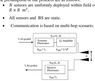
The energy model in [11] and represented in Fig. 1 is used in SEPCS. According to this model, the energy consumed to transmit L−bit message over a distance d, is calculated as follows:
𝐸𝑇𝑥(𝐿, 𝑑) = {
𝐿. 𝐸𝑒𝑙𝑒𝑐+ 𝐿. 𝜖𝑓𝑠. 𝑑2 𝑖𝑓 𝑑 ≤ 𝑑0
𝐿. 𝐸𝑒𝑙𝑒𝑐+ 𝐿. 𝜖𝑚𝑝. 𝑑4 𝑖𝑓 𝑑 > 𝑑0
, (5) Here, 𝐸𝑒𝑙𝑒𝑐 is the energy consumed per bit to execute the transmitter or the receiver circuit, 𝜖𝑓𝑠 and 𝜖𝑚𝑝 depends on the transmitter amplifier model. By equating the two expressions at d = d0, we have d0= √
ϵfs
ϵmp. To receive an L−bit message the radio expends ERx= L. Eelec.
The presumption of our protocol are as follows:
• 𝑁 sensors are uniformly deployed within field of area
𝑅 × 𝑅 𝑚2,
• All sensors and BS are static.
• Communication is based on multi-hop scenario.
Figure 1. The energy consumption model.
2.2 Optimal number of clusters
For simplicity, we assume that BS is located at field center and the distance between any node to the BS or its CH is less than or equal to 𝑑0. Then, the energy consumed by CHs during one round is computed as:
𝐸𝐶𝐻= ( 𝑁
𝐶− 1) 𝑌𝐸𝑒𝑙𝑒𝑐+ 𝑁
𝐶𝑌 + 𝑌𝐸𝑒𝑙𝑒𝑐+ 𝑌𝜖𝑓𝑠𝑑𝐵𝑆 2 , (6) Here, clusters number is 𝐶, compressed data is 𝑌 and 𝑑𝐵𝑆 is the average distance between CH and BS. The energy consumed by CMs is computed as:
𝐸𝑛𝑜𝑛𝐶𝐻= 𝐿. 𝐸𝑒𝑙𝑒𝑐+ 𝐿. 𝜖𝑓𝑠𝑑𝐶𝐻2 , (7) Here, 𝑑𝐶𝐻 is the average distance between CMs and their CH. the occupied area by each cluster can be computed using Euclidian distance as 𝐴 = 𝑅2
International Journal of Communication Networks and Information Security (IJCNIS) Vol. 11, No. 1, April 2019
𝑑𝐶𝐻2 = ∫ ∫(𝑥2+ 𝑦2)𝜌(𝑥, 𝑦) 𝑑𝑥𝑑𝑦
= ∫ ∫ 𝑟2𝜌(𝑟, θ)𝑟𝑑𝑟𝑑θ, (8) We assume that the area is a circle with radius 𝜂 = 𝑅 √𝜋𝐶⁄ ,
𝜌(𝑟, θ) is constant and the density 𝜌 is uniform where 𝜌 = (1 (𝑅⁄ 2⁄𝐶), 𝑑
𝐶𝐻2 can be simplified as follows:
𝑑𝐶𝐻2 = ∬ ∫(𝑥2+ 𝑦2)𝜌(𝑥, 𝑦) 𝑑𝑥𝑑𝑦
= 𝜌 ∫ ∫𝑅 √𝜋𝐶⁄ 𝑟3𝑑𝑟𝑑θ 𝑟=0
2𝜋
θ=0 =
𝑅2
2𝜋𝐶, (9) In each round, the energy consumed by every cluster is computed as:
𝐸𝑐𝑙𝑢𝑠𝑡𝑒𝑟≈ 𝐸𝐶𝐻+ 𝑁
𝐶𝐸𝑛𝑜𝑛𝐶𝐻, (10) In each round, the total energy consumed by all sensor nodes is:
𝐸𝑡𝑜𝑡 = 𝐶𝐸𝑐𝑙𝑢𝑠𝑡𝑒𝑟= 𝑌(𝑁(1 + 𝐸𝑒𝑙𝑒𝑐) + 𝐶𝜖𝑓𝑠𝑑𝐵𝑆2 ) +
𝑁𝐿(𝐸𝑒𝑙𝑒𝑐+ 𝜖𝑓𝑠𝑑𝐶𝐻2 )), (11)
Differentiating 𝐸𝑡𝑜𝑡 with respect to 𝐶 and equating to zero, the optimal number of clusters is computed as follows:
𝐶𝑜𝑝𝑡= √ 𝑁𝐿 2𝜋𝑌
𝑅 𝑑𝐵𝑆= √
𝑁𝐿 2𝜋𝑌
2
0.765, (12)
𝑑𝐵𝑆 is the average distance between CH to BS is:
𝑑𝐵𝑆= ∫ √𝑥2+ 𝑦2 1𝐴𝑑𝐴 = 0.765 𝑅
2, (13) If the distance of a large number of nodes to the BS is bigger than 𝑑0then, follow same analysis as in [5]:
𝐶𝑜𝑝𝑡 = √ 𝑁𝐿 2𝜋𝑌√
𝜖𝑓𝑠
𝜖𝑚𝑝 𝑅
𝑑𝐵𝑆2 , (14) The optimal probability of a node to become a CH, 𝑝𝑜𝑝𝑡, can be computed as follows:
𝑝𝑜𝑝𝑡= 𝐶𝑜𝑝𝑡
𝑁 , (15) The optimal number of clusters is very important issue. The work in [10] cleared that the energy consumed in the network per round will be exponentially increased if the optimal number of clusters are not found, either when the number of clusters is more than the optimal number of clusters; where the total routing traffics within each cluster will be reduced because of fewer members; however, more clusters will result in multi-hop transmissions from CHs to BS and every CH will receive data from fewer members this will decrease the local data aggregation and increase the communications among the CHs, or when the number of clusters is less than the optimal number of clusters; where some nodes in the network have to send their sensed data far to reach CH, causing the global energy in the system to be large.
2.3 Cluster head election phase
Finding the optimal number of clusters implies the optimal selection of a node to be a CH. The cluster is optimal if the energy consumption is well distributed among all sensors and the total energy consumption is minimized. Since energy consumption of the CHs is approximately high, so the residual energy of sensor is the main criteria for CH selection. In addition, data aggregation can save considerable energy when
the source nodes constructing a cluster when these nodes in a nearly small region while the BS is far away from the source nodes, because sensors require much less energy for transmitting data to the CH than transmitting it directly to the BS when the BS is located at a remote distance. Therefore, it is reasonable to derive that the closer source nodes within a cluster, the lower energy they need to consume to transmit data.
According to the discussion above, the selection of CHs in SPCS will be based on concentration degree and residual energy of sensor nodes.
Definition 1: Given WSN of 𝑁 the concentration degree of a node 𝑖, 𝐷𝑟(𝑖) (𝑖 = 1, 2, … , 𝑁)is the number of sensor nodes that can sense during the 𝑟𝑡ℎ round.
Definition 2: Election weight of node 𝑖 in round r 𝑊(𝑖, 𝑟) is defined as:
𝑊(𝑖, 𝑟) = 𝛼𝐸𝑖𝑟
𝐸̅𝑟+ (1 − 𝛼) 𝐷𝑟(𝑖)
𝑝𝑜𝑝𝑡, (16) Here, 𝛼 = 1
1+𝛽 is an adaptive factor to regulate the effect of residual energy and concentration degree on the election weight, 𝛽 =𝐸𝑖𝑟
𝐸̅𝑟 denotes the average residual energy of node 𝑖 in round 𝑟, 𝐸𝑖 is the initial energy of node 𝑖 and 𝐸̅𝑟 is the average residual energy of network in rth round. With the reduction of residual energy, α will gradually increase to adapt to decrease the number of effective sensors in WSN.
2.4 Setup phase
• Step 1: During the initialization, every sensor computes its concentration degree and ticks its level as level 1.
• Step 2: Initialization phase: In “CH selection” messages, 𝐸̅𝑟 will be broadcasted by BS. Every node
𝑖compares its 𝐸𝑖𝑟with 𝐸̅𝑟. If 𝐸𝑖𝑟≥ 𝐸̅𝑟, 𝑖computes its
𝐷𝑟(𝑖) and 𝐸
𝑖𝑟, and sends the weight with its ID to the BS for CH selection in “CH selection” message. Otherwise, a node 𝑖 abandons CH selection, and selects to join a CH later.
• Step 3 BS ticks its level as level 1, selects 𝐶𝑜𝑝𝑡 sensors that have maximum selection weight as CHs. Every selected CHs broadcasts to report its neighbors that it has been selected as a CH.
• Step 4 If a sensor is selected as a CH, it will broadcast “re-join” messages to each non-CH sensor. After receiving the broadcast message, every non-CH selects its nearest CH according to the received signal strength and then notifies the CH by transmitting a join message.
• Step 5 CH sets up TDMA schedule and sends it to its CMs.
2.5 Data transmission phase
After forming the clusters and receiving the TDMA schedule, the transmission phase of the data can start. The sensors periodically gather the data samples 𝑋 =
[𝑥1, … , 𝑥𝑁], and send it during their allocated transmission time to the CH.
Here, 𝑆 ∈ ℝ𝑁 is the transform coefficient vector which contains 𝐾(𝐾 ≪ 𝑁) nonzeros, and 𝐷 is the DWT basis. After receiving all data, CHs compress the gathered data using CS. The received data vector at CH can be rewritten as:
𝑌 = 𝛷𝑋 = 𝛷𝛹𝑆, (18) Here, Φ is the sampling matrix whose entries are
i. i. d Gaussian with zero mean and unit variance. Subsequently CHs transmit measurements Y to the BS independently. Finally, the BS decodes the networked data X
from Y.
3.
Simulation Results
In this section, using Matlab and Sparselab toolbox [17], we prove the efficiency of the proposed protocol and compare the results with the baseline algorithms in terms of energy consumption and network lifetime and the stability period. The parameters of the simulation are listed in table. I.
Table 1. Simulation parameters.
Description Parameter Value
No. of nodes N 1000
Initial energy 𝐸0 0.5
Location of the BS BS (50,50)
Data packet size L 4000 bits
Network area 𝑅 × 𝑅 200 × 200 𝑚2
Transmit amplifier if 𝐝𝐁𝐒≤
𝐝𝟎
𝜖𝑓𝑠 10 𝑝𝐽/(𝑏𝑖𝑡 ∗ 𝑚2)
Transmit amplifier if 𝐝𝐁𝐒≥
𝐝𝟎
𝜖𝑚𝑝 0.0013 𝑝𝐽/(𝑏𝑖𝑡
∗ 𝑚4)
Threshold distance 𝑑0 87.7058 𝑚
No. of nonzero Coefficients 𝐾 10
No. of measurements 𝑀 50
Propagation loss factor 𝛾 2
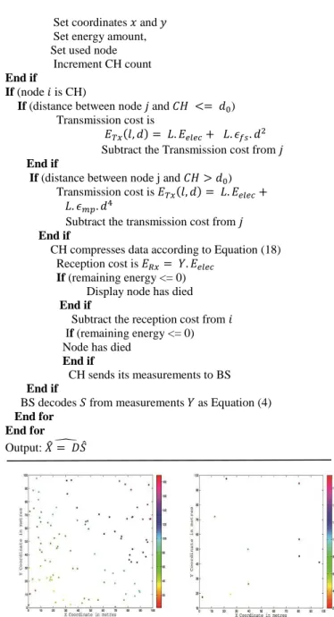
We choose the number of nonzero coefficients K = 10 such that K<M≪N. Fig. 2(a) shows Network topology comprised of 100 sensor nodes corresponds to DWT basis. The networked data shown in Fig. 2(b) can be presented with K = 10 nonzero coefficients after DWT transform.
3.1 Performance metrics
In our simulation, we used the following metrics to validate the performance of the proposed protocol SEPCS:
• Network lifetime: is the time interval from the start of operation of WSN until the death of all sensor nodes.
• Throughput: is the rate of data sent from CHs to BS over the lifetime of the network.
• Stability period: is the time interval from the start of network operation until the death of the first alive node.
Algorithm 1 Stable Election Protocol using CS
Input Parameters: Table 1 listing the input parameters of this algorithm
For each round
BS broadcasts the average residual energy of network
For each node
Node calculates its concentration degree as in Def. 1
If (residual energy of node ≥ average residual energy of WSN)
Node computes its election weight as Equation (16) BS chooses CHs with maximum election weight
Set coordinates 𝑥 and 𝑦
Set energy amount, Set used node
Increment CH count
End if
If (node 𝑖 is CH)
If (distance between node 𝑗 and 𝐶𝐻 <= 𝑑0) Transmission cost is
𝐸𝑇𝑥(𝑙, 𝑑) = 𝐿. 𝐸𝑒𝑙𝑒𝑐+ 𝐿. 𝜖𝑓𝑠. 𝑑2 Subtract the Transmission cost from 𝑗
End if
If (distance between node j and 𝐶𝐻 > 𝑑0) Transmission cost is 𝐸𝑇𝑥(𝑙, 𝑑) = 𝐿. 𝐸𝑒𝑙𝑒𝑐+ 𝐿. 𝜖𝑚𝑝. 𝑑4
Subtract the transmission cost from 𝑗
End if
CH compresses data according to Equation (18) Reception cost is 𝐸𝑅𝑥= 𝑌. 𝐸𝑒𝑙𝑒𝑐
If (remaining energy <= 0) Display node has died
End if
Subtract the reception cost from 𝑖
If (remaining energy <= 0) Node has died
End if
CH sends its measurements to BS
End if
BS decodes 𝑆 from measurements 𝑌 as Equation (4) End for
End for
Output: 𝑋̂ = 𝐷𝑆̂̂
Figure 2. Sparsity of networked data in a DWT basis.
3.2 Energy consumption
International Journal of Communication Networks and Information Security (IJCNIS) Vol. 11, No. 1, April 2019
Figure 3. Average energy consumption.
3.3 Network lifetime
In WSNs, total survival network lifetime is considered as one of the most important metric. In the second test, the network lifetime of SEPCS is computed and compared with existing protocols. Fig. 4 shows the network lifetime of LEACH, SEP, WEP and SEPCS. It shows the number of alive nodes with respect to number of rounds. From the figure, both the death time of first node and the death time of last node of SPECS takes place later than those of LEACH, SEP and WEP. Also, WEP performs better than SEP because WEP uses chain among CHs instead of all nodes in order to alleviate the excessive delay to transmit data to BS. As well, SEP performs better than LEACH, the reason is every sensor node independently elects itself as a CH based on its initial energy relative to that of other nodes. However, the network will be alive for a longer period of time with our proposed protocol compared with LEACH and SEP because SEPCS efficiently compresses data using CS, consequent to this compression; the total network energy consumption is minimized. In addition, SEPCS uses residual energy and degree concentration of sensors to select CHs. where sensors with high election weight has greater chances to be a CH..
Figure 4. Number of alive nodes over rounds.
3.4 Throughput
In the third test, the overall throughput is evaluated in terms of number of received messages exchanged at BS using LEACH, SEP, WEP and SEPCS. Fig. 5 shows that the overall throughput of SEPCS is significantly greater than those of LEACH, SEP and WEP protocols because SEPCS efficiently compresses data using CS and optimizes energy usage to reduce storage space and energy consumed, and also the CHs selection mechanism is based on the residual energy and the concentration degree of sensors.
Also, it shows that the throughput of WEP is better than SEP because WEP uses greedy algorithm to make a chain among the selected CHs for achieving more throughput gain. As well
as the throughput of SEP is significantly larger than that of LEACH because SEP guarantees CHs in more rounds.
Figure 5. Throughput of the network. 3.5 Stability
In WSNs, the stability period is crucial for many applications where the feedback from the sensors must be reliable. In the fourth test, we study the sensitivity of SEPCS protocol and compare the results with other protocols in terms of the stability period length. Fig. 6 shows the stability period length of LEACH, SEP, WEP and SEPCS. It shows that SEPCS outperforms WEP by up to 19.6%, SEP by up to 23.4% and LEACH by up to 39.1%, i.e., the proposed SEPCS is significantly prolongs the stability period compared to LEACH, SEP and WEP. This is because SEPCS efficiently compresses data to a great ratio and the selection of CHs is carried in an optimal way, therefore, stability period of SEPCS is enhanced which is the main requirement for the lifetime of the WSN.
Figure 6. Network stable period.
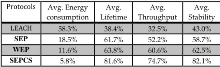
Table1.Average percentage of energy consumption, lifetime, throughput and stability in leach, SEP, WEP and SEPCS.
Protocols Avg. Energy
consumption
Avg. Lifetime
Avg. Throughput
Avg. Stability
LEACH 58.3% 38.4% 32.5% 43.0%
SEP 18.5% 61.7% 52.2% 58.7%
WEP 11.6% 63.8% 60.6% 62.5%
SEPCS 5.8% 81.6% 74.7% 82.1%
4.
Conclusion
extends the stability period and the lifetime of the network compared to LEACH, SEP and WEP.
References
[1] M. Khedr and W. Osamy, “Effective Target Tracking Mechanism in a Self- Organizing Wireless Sensor Network,” Journal of Parallel and Distributed Computing, Vol. 71, pp. 1318-1326, 2011.
[2] M. Khedr and W. Osamy, “Minimum perimeter coverage of query regions in heterogeneous wireless sensor networks,” Information Sciences, Vol. 181, pp. 3130- 3142, 2011. [3] M. Khedr and W. Osamy, “A Topology Discovery Algorithm
For Sensor Network Using Smart Antennas,” Computer Communications Journal, Vol. 29, pp. 2261-2268, 2006. [4] M. Khedr, W. Osamy, and Dhrama P. Agrawal, “Perimeter
Discovery in Wireless Sensor Networks,” J. Parallel Distrib. Comput. Vol. 69, pp. 922-929, 2009.
[5] M. Khedr and W. Osamy, “Target tracking Mechanism for Cluster Based Sensor Networks,” Applied Mathematics and Information Science Journal, Vol. 1, No. 3, pp. 287- 303, 2007. [6] M. Khedr, “Tracking Mobile Targets using Grid sensor networks,” GESJ: Computer science and Telecommunications, Vol. 3, No. 10, pp. 66-84, 2006.
[7] H. Yang and B. Sikdar, “Optimal CH Selection in the LEACH Architecture, IEEE International Conference on Performance, Computing, and Communications, pp. 93-100, 2007.
[8] N. M. A. Latiff, C. C. Tsimenidis and B. S. Sharif, “Performance Comparison of Optimization Algorithm for Clustering in Wireless Sensor Networks, IEEE International Conference on Mobile Adhoc and Sensor Systems, pp. 1-4, 2007.
[9] Z. Zhang and X. Zhang., “Research of Improved Clustering Routing Algorithm Based on Load Balance in Wireless Sensor Networks, IET International Communication Conference on Wireless Mobile and Computing, pp. 661-664, 2009.
[10]W. R. Heinzelman, A. Chandrakasan, and H. Balakrishnan, “Energy-efficient communication protocol for wireless microsensor networks, Proceedings of the 3rd Hawaii International Conference on System Sciences, pp. 1-10, 2000. [11]W. R. Heinzelman, A. Chandrakasan, and H. Balakrishnan, “An
Applocation-Specific Protocol Architecture for Wireless Microsensor Networks, IEEE Transactions on Wireless Communications, Vol. 1, No. 4, pp. 662-666, 2002.
[12]G. Smaragdakis, I. Matta and A. Bestavros, “SEP: A Stable Election Protocol for Clustered heterogeneous wireless Sensor Networks”, Second International Workshop on Sensor and Actuator Network Protocols and Applications (SANPA-04), 2004.
[13]E. J. Cand´es, and M. B. Wakin, “An introduction to compressive sampling”, IEEE Signal Process. Mag., Vol. 25, No. 2, pp. 21-30, 2008.
[14]O. Younis and S. Fahmy, “HEED: A Hybrid Energy Efficient Distributed Clustering Approach for Ad Hoc Sensor Networks”, EEE Transactions on Mobile Computing, Vol. 3, pp. 660-669, 2004.
[15]S. Bandyopadhyay, E. J. Coyle, “Minimizing communication costs in hierarchically clustered networks of wireless sensors,” Computer Networks, Vol. 44, No. 1, pp. 1-16, 2004.
[16]D. Donoho, V. Stodden and Y. Tsaig, Sparselab [Online]. Available:
[17]http://sparselab.stanford.edu/
[18]Md. G. Rashed, M. H. Kabir and S. E. Ullah, “WEP: An Energy Efficient Protocol for Cluster Based Heterogeneous Wireless Sensor Network”, International Journal of Distributed and Parallel Systems (IJDPS), Vol. 2, No. 2, 2011.
[19]W. Osamy, A. M. Khedr, A. Aziza, and A. El-Sawya, “Cluster-Tree Routing Scheme for Data Gathering in Periodic Monitoring Applications, IEEE Access, Vol. 6, Page(s): 77372-77387.
[20]W. Osamy, A. Salim, and A. M. Khedr, “An Information Entropy Based-Clustering Algorithm in Heterogeneous Wireless Sensor Networks, accepted in wireless networks, Springier, doi.org/10.1007/s11276- 018-1877-y-0123456789, 2018.
[21]A. Aziz, K. Singh,W. Osamy, and A. M. Khedr, Effective Algorithm for Optimizing Compressive Sensing in IoT and Periodic Monitoring Applications, Journal of Network and Computer Applications, vol. 126, pp. 12-28, 2019
[22]D. M. Omar, “ERPLBC: Energy Efficient Routing Protocol for Load Balanced Clustering in Wireless Sensor Networks,”0 Ad Hoc & Sensor Wireless Networks, Vol. 42, pp. 145-169, 2018.
[23]D. M. Omar, and A. M. Khedr, D. P. Agrawal Optimized Clustering Protocol for Balancing Energy in Wireless Sensor Networks, International Journal of Communication Networks and Information Security (IJCNIS) Vol. 9, No. 3, pp. 367-375, December 2017.
[24]W. Osamy, A. M. Khedr, An algorithm for enhancing coverage and network lifetime in cluster-based Wireless Sensor Networks, International Journal of Communication Networks and Infor- mation Security (IJCNIS) Vol. 10, No. 1, pp. 1- 9, April 2018.