Congestion Controlled WSN using Genetic Algorithm
with different Source and Sink Mobility Scenarios
Anu Verma
ECE Department Chandigarh University Gharaun, Mohali, India
Nitin Mittal
ECE Department Chandigarh University Gharaun, Mohali, India
ABSTRACT
Wireless Sensor Networks are extremely densely populated and have to handle large bursts of data during high activity periods giving rise to congestion which may disrupt normal operation. It usually occurs when most of the data packets follow one route to reach from source to destination. Thus, there is a need of some new approach which could control congestion to meet increasing traffic demand and improved utilization of existing resources. Chance of congestion increases when both source and sink node are mobile. Due to mobility of source or sink, there is a need of determining optimal path every time when source or sink changes its position. So selection of optimal path is necessary in order to mitigate chance of congestion in the network. This paper employs new genetic algorithm based approach to determine an optimal path from source to destination for different scenarios of source or/and sink node mobility. Concept of connection value and localization region has been employed to determine an optimal path each time the data packet is being sent. An optimal path is the path that has minimum number of connections. In order to send the data packet from source to destination, there is requirement of genetic algorithm that automatically controls congestion. Simulations are performed for different scenarios of source or/and sink mobility. Significant improvements have been observed in terms of congestion value for genetic algorithm. Simulations results determine best route with minimum connection value by incorporating genetic algorithm.
Keywords
Genetic Algorithm, Connection value, Optimization, Wireless sensor network
1.
INTRODUCTION
A wireless sensor network comprises of a large number of sensor nodes that are connected to each other wirelessly in an adhoc manner [1]. It has increased the capability of humans for exploration, monitoring and controlling the physical world. Wireless sensor network differs from traditional wired networks in terms of resources like unlimited memory, power supply, adequate computational capabilities and communication range [3]. On other hand, wireless sensor networks are resource constraint distributed systems having low energy, low bandwidth and small communication range. This resource constrained nature of wireless sensor network imparts various challengeslike maximizing lifetimeof nodes, heterogeneity and scalability of the sensor nodes, responsiveness, energy efficiency, robustness, self adaptation and configuration of sensor nodes etc. [4].
For improving the performance of wireless sensor network, these challenges are subjected to scrutinize. The performance of wireless sensor network can be improved by pertinent
resource utilization. It can be enhanced by centering on various factors which are involved in wireless sensor network operations. The factor which highly influences the resources of WSN is communication. This communication includes optimal selection of route, maintenance of route and various other computations to compete with prospect of user and also to ensure network performance [5]. Selection of route of each message in communication framework results in network delay if long route is selected. It also degrades the lifetime of the network if short route is selected which results in depletion of batteries [6]. Besides this, superfluous load on the network causes congestion which is the prime reason for degradation of application quality.
In this paper, the factor based on congestion i.e. connection value of nodes is selected for the determination of optimal path. Genetic Algorithm is used to find an optimal path every time before sending data packet which reduces chance of congestion in the network. Moreover, information received at destination is of use only if the origin of the source, i.e., location of the sensor node is known. Moreover, location of all randomly deployed sensor nodes is also required to determine the route for information passing. In the present work, some localization regions have been assumed. Nodes present in these localization regions are assumed to be localized. The rest of the paper is structured as follows: Section 2 describes the literature review, section 3 presents the proposed method, simulation results have been shown in section 4 while section 5 concludes the paper and section 6 presents future research directions.
2.
LITERATURE SURVEY
have been found by utilizing position of anchor nodes. Angelo F. Assis et al. proposed a genetic algorithm approach for localizing the nodes by choosing the criteria of minimum cost as a parameter [15]. In wireless sensor networks, main paramount issue is localization of nodes. Beacon nodes are used for finding the location of unknown nodes. Genetic algorithm identifies minimum set of anchor nodes for locating every sensor belonging to network. Simulation results prove better results than greedy sweep method. In [29] author narrates a tree forming scheme for controlling congestion in wireless sensor network. Topology control algorithms are employed in order to reduce the number of active nodes and ease the transportation of data from source to sink. Author presented source-based trees, shared-, core-based trees (sink-based trees) and a naive source-(sink-based tree structure and evaluates them under resource and traffic congestion control methods. Simulation results show that not only sink-based trees, but also source-based trees can provide efficient and effective topology control solutions, which are, of course, application specific.
From the previous literature, it was observed that no work has been done for a scenario where both source and sink node are moving.
3.
PROPOSED WORK
In the proposed work genetic algorithm has been implemented for the determination of optimal path where chances of congestion are negligible. To find an optimal path, the concept of localization and connection value of nodes has been used. Genetic Algorithm has been applied to different scenarios of source or/and sink mobility. Whenever source or sink changes its position with respect to its initial value, optimal path is found.
3.1
Assumption of Localization Regions
In wireless sensor network, accurate location of sensor nodes is highly desirable for sending data message from source to destination. In proposed algorithm, concept of localization has been used for designing the network. Localization of the nodes refers to nodes which know their location in the network [13]. It is obvious that if the information passes through nodes which know their location in the network, then information can be reliably transferred from source to destination. Data transmission through reliable nodes reduces the chance of congestion in the network. However achieving localization is not a prime concern.
In the present work, if any node comes in range of at least three beacon nodes, then that node is said to be localized [13] which means localization region is the common area of three beacon nodes. In the present work, some localization regions have been assumed. In pre-defined area, sensor nodes are randomly deployed. Nodes that come inside localization regions are assumed to be localized and know their location. Only nodes present in localization regions are used for determining an optimal path from source to destination.
3.2
Calculation of Connection Value of
nodes
When any node is having connection with maximum number of nodes, then, there is greater chance of having congestion through this node [28]. For calculating connection value, particular threshold range value is given to all nodes for determining number of neighborhood nodes. For example, consider a node in localized region, having range of 10m, then, it calculates its distance with all nodes of localized
region. The count of nodes which came under predefined range is considered as its connection value. Connection value is defined as number of localized nodes that come inside the
range of any localized node.
In present work, only connection value of those nodes are calculated which come inside localization regions. Suppose, for example, any localized node is connected with five localized nodes then connection value of that node is considered as five. Similarly, connection value of all nodes present in different localization regions is calculated.
3.3
Genetic Algorithm Approach
Main objective of proposed work is to select the reliable paths in the network for reducing the congestion in the network. And to achieve this, an optimization technique called genetic algorithm is used. The aim of the genetic algorithm in present work is to minimize the objective function that is to be optimized. The following is the process of GA
3.3.1
Population Initialization
Population initialization is done by randomly selecting the paths (intermediate nodes) from localization regions. If no node comes inside any of the localization regions, then population is again generated until node comes inside the localization region.
3.3.2
Determining Fitness Function
Fitness function=
with the constraint that cv ≠ 0 where cv is connection value and N denotes total number of nodes existing in any route from particular source to particular destination. Connection value is the number of localized nodes that comes inside the range of any localized node.
3.3.3
Calculating Fitness value of each individual
Fitness function is calculated by arithmetic sum of the connection value of the nodes existing in the paths between source and destination. It will obviously lead to congestion controlled paths if different paths are chosen having minimum fitness value and thus reducing the overall congestion of the network.
3.3.4
Crossover and Mutation
Crossover is the process which combines genes of two individuals to form one parent.The principle is to choose two parents whose genetic code will be recombined with the probability of variable crossover probability pm to create two new off springs. For this, crossover rate is selected as 0.6. For selection process, all individuals are sorted in accordance with fitness value. Fittest individuals are selected for crossover and mutation. We pick the parents from the beginning and from the end of list, coming towards the middle. In this way, we guarantee that worst parent will be recombined with best parent generating most diverse results. Regarding recombination, we generate a random number and based on it, crossover between two parents is performed. After crossover operation, fitness value of each route is calculated. Firstly fitness value of initial population is calculated, then fitness value after crossover is calculated. If the fitness value obtained after crossover is less than the fitness value of initial population then population after crossover is retained otherwise initial population path before crossover is selected.
that localization region. Suppose other two nodes present in that localization regions are 11th and 15th. Then 7th node can randomly be replaced by 11th or 15th node. Mutation rate is selected as 0.04. Then fitness value obtained after crossover, initial population and after mutation is compared. If the fitness value obtained after mutation is less than from both initial population and crossover process than population after mutation is retained. After maximum number of iterations has been reached, route is selected with minimum fitness value.
3.3.5
Terminating Condition
Genetic Algorithm terminates after reaching a fixed no. of generations.
4.
SIMULATION RESULTS
To control congestion in wireless sensor network, genetic algorithm based approach is employed using MATLAB simulation software. To evaluate the performance of proposed algorithm, simulations are performed on different scenarios of source or/and sink mobility. Simulation results are presented in this paper in terms of fitness value. Fitness value decides the best suitable path for data routing. We termed fitness value as congestion value as number of connections is related to congestion. Optimal path is determined by using GA having minimum number of connections.
For the following configuration of the network, infrastructure details are given in the table below:
Table 1. Architectural details of Wireless sensor Network
Wireless Sensor network Number of nodes 50 , 250 Total area of network 110x100 m2 Area of source and sink node
assignment
10x100 m2
Number of localization
regions
4
Number of mobility rounds of position variance of source or/and sink
10
Transmission Range of each node
30m
Various parameters taken for Genetic Algorithm are: (1) Number of Iterations-50 (2) Population Size-20 (3) Crossover rate-0.6 (4) Mutation Rate-0.04
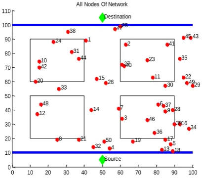
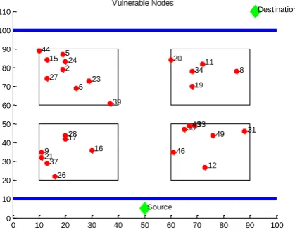
[image:3.595.334.539.76.260.2]Fig 1 shows the randomly deployed nodes in the predefined area. All deployed nodes are red in color except source and destination node. Green nodes are designated as source and destination node. Fig 2 shows vulnerable nodes i.e. nodes which come under localization regions.
[image:3.595.330.537.77.507.2]Fig 1: Randomly deployed nodes
Fig 2: Vulnerable nodes
4.1
Fixed Source and Sink Scenario
By varying number of nodes, simulations have been conducted for the scenario where both source and sink node are fixed.
Fig 3 shows comparison between value before applying genetic algorithm and value obtained after applying genetic algorithm. Actual represents minimum value before applying genetic algorithm and Proposed represents minimum value obtained after applying genetic algorithm. Simulation represents best possible path having minimum number of connections.
S-12-9-31-2-D
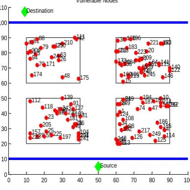
The main purpose of proposed Genetic Algorithm is to determine least congestion path rather than determining shortest path. Then, simulation has been conducted by increasing the complexity of a system by deploying 250 nodes. Fig 4 determines vulnerable nodes and Fig 5 shows comparison between actual and proposed value for 250 nodes.
In Fig 4, each node is connected to a several number of other nodes as more number of nodes comes within the range of the particular nodes. In plotting such a network, the complexity of the network increases as more powerful transmission systems will be required.
0 10 20 30 40 50 60 70 80 90 100
0 10 20 30 40 50 60 70 80 90 100 110
1
2
3
4 5
6 7
8
9 10
11
12
13 14
15
16
17
18 19
20
21
22 23
24
25
26 27
28 29 30 31
32 33
34 35
36 37 38
39 40
41
42
43
44
45
46 47
48
49
50 All Nodes Of Network
Source Destination
0 10 20 30 40 50 60 70 80 90 100
0 10 20 30 40 50 60 70 80 90 100 110
12 48
3
6 9 28
36 37
39 46 10
20 24
31
42
44
2
11 23
2740
41
[image:3.595.333.534.294.503.2]Fig 3: Comparison of Actual and Proposed with GA congestion value for fixed source and sink
Fig 4: Vulnerable nodes for fixed source and sink
Fig 5: Comparison of Actual and Proposed with GA congestion value for fixed source and sink
In Fig 4, each node is connected to many other nodes so it becomes very difficult to propose a path which may have the best fitness value. So the genetic algorithm comes as a big rescue in such scenarios with increased number of nodes which helps us to determine the best fit solution. The beauty
of the system that we have designed is that it can be extended to as many numbers of nodes as required and it helps us to find the best possible path for routing of data from source to destination.
56 186 63 98
4.2
Fixed Source and Sink Moving
[image:4.595.76.271.284.450.2]By varying number of nodes, simulations have been conducted for the scenario where source is fixed and sink is moving. For this scenario, number of mobility rounds for position variance of sink has been taken as 10. The location of sink is changing from one position to another after completing all iterations of Genetic Algorithm at that position. Fig 6 represents vulnerable nodes at initial position of sink for 50 nodes and Fig 7 represents graph between actual and proposed fitness or congestion value.
Fig 6: Vulnerable nodes at 1st position of sink
Fig 7: Comparison of Actual and Proposed with GA congestion value
Simulation represents 10 optimal paths for each position variance of sink with respect to its initial value. Below is table representing 10 optimal paths.
1 2 3 4
0 1 2 3 4 5 6 7 8
Comparison Of Actual ANd Proposed Achieved Congestion
C
o
n
g
e
s
ti
o
n
V
a
lu
e
Actual Proposed
Before GA After GA
0 10 20 30 40 50 60 70 80 90 100
0 10 20 30 40 50 60 70 80 90 100 110
2
6 9
15 27
37
40 41
46 56
74 79 84 96
100
105 110
118 119 133
135 140
142 146 174181
188 193 195
210
214 237
1 4
5 10
11 18 20
26
29 38
42
44 48
60 66
68 91 99
101 102 124
125 128
149 165
166 173
175 180
186 200
207217 211 227 249
7 12
25
28 35
43
58
63 70 76
80 82
103 108 115 116
144
148 154
156 167
171
176 190
203
206
209 234
238 239 242
16 19
53 64
65
69 75
77
88 98
121 129 131
136
137 155
157 158
161 178 192
194 196
221 246
Source Destination Vulnerable Nodes
1 2 3 4
0 5 10 15 20 25 30 35 40
Comparison Of Actual ANd Proposed Achieved Congestion
C
o
n
g
e
s
ti
o
n
V
a
lu
e
Actual Proposed
Before GA
After GA
0 10 20 30 40 50 60 70 80 90 100
0 10 20 30 40 50 60 70 80 90 100 110
9 16
17 21
26 28
37 12
304333 31
46 49 2
5
6 15
23 24 27
39 44
8 11
19 20
34
Source
Destination Vulnerable Nodes
1 2 3 4
0 2 4 6 8 10 12
Comparison Of Actual ANd Proposed Achieved Congestion
C
o
n
g
e
s
ti
o
n
V
a
lu
e
Actual Proposed
Before GA
[image:4.595.328.545.462.651.2] [image:4.595.68.279.486.674.2]Table 2. Optimal route table for each position variance of sink
Variation in position of
Sink Optimal Path
1st S-28-49-27-19-D
2nd S-28-49-39-8-D
3rd S-26-31-2-24-D
4th S-16-31-39-8-D
5th S-28-31-39-20-D
6th S-16-46-2-34-D
7th S-17-43-5-34-D
8th S-16-31-39-8-D
9th S-17-31-39-11-D
10th S-37-30-2-34-D
At each position of sink, optimal path determined is the path having minimum fitness or congestion value. Optimal path specified after applying genetic algorithm at each position variance of sink can be similar or distinct depending upon number of connections.
By increasing the complexity of the system with increasing number of nodes from 50 to 250, system is still able to compute path with best fitness value. For 250 nodes scenario, only vulnerable nodes and comparison between actual and proposed value have been shown to determine effectiveness of proposed algorithm.
[image:5.595.48.289.82.296.2]Fig 8 shows that when the number of nodes is increased the system still works well and is able to find out an optimized solution which is the best optimal path for transferring of data from source to destination. Fig 9 shows comparison between actual value before applying genetic algorithm and proposed value after applying genetic algorithm. It depict that number of connections are reduced from 34 to 15. Also, 10 optimal paths have been determined for each position variance of source with respect to its initial value.
[image:5.595.48.290.88.294.2]Fig 8: Vulnerable nodes
Fig 9: Comparison of Actual and Proposed value
4.3
Moving Source and Fixed Destination
[image:5.595.332.532.350.519.2]Fig 10 determines vulnerable nodes at initial position of source for the scenario of 50 nodes and Fig 11 shows comparison of congestion value before and after applying genetic algorithm.
Fig 10: Vulnerable nodes at initial position of source
Fig 11: Comparison of Actual and Proposed with GA congestion value
0 10 20 30 40 50 60 70 80 90 100
0 10 20 30 40 50 60 70 80 90 100 110
23
25 28
31 36 49 55
75 91
104 112
118 127
134 139
142
157
160 167 180
181
197 201
205
222 225
230
241
243 1
2 4
10
34 47
54
59
65 68
74 84
98 108
113
114 124
125 126 148
149 161
185 186 187 194
199
202
212 214
217 219
249 5
26 42 43
48
61 63
70 79
8188
94
111
171
174 175
177 206
210
244 250
15 20 30
45 60
64 73 7677 103
106 115 120
122 140 141
146 151 159 166
169 173
183
184
193 196
209 213
215 221 223
236 245 248
Source Destination
Vulnerable Nodes
1 2 3 4
0 1 2 3 4 5 6 7 8 9 10 11
Comparison Of Actual ANd Proposed Achieved Congestion
C
o
n
g
e
s
ti
o
n
V
a
lu
e
Actual Proposed
[image:5.595.76.270.542.735.2] [image:5.595.329.533.561.735.2]Table 3. Optimal route table for each position variance of source
Variation in position of
Source Optimal Path
1st S-28-48-2-30-D
2nd S-35-48-32-5-D
3rd S-39-46-19-16-D
4th S-35-31-39-1-D
5th S-28-18-32-9-D
6th S-24-18-32-30-D
7th S-24-26-32-16-D
8th S-24-33-2-5-D
9th S-39-26-19-30-D
[image:6.595.53.285.95.700.2]10th S-35-7-4-16-D
Fig 12: Vulnerable nodes
Fig 13: Comparison of Actual and Proposed with GA congestion value
For this scenario, number of mobility rounds for position variance of source has been taken as 10. The location of source is changing from one position to another after completing all iterations of Genetic Algorithm at that position. The Fig 12 determines vulnerable nodes for scenario of 250
nodes and Fig 13 determines comparison between actual and proposed value.
4.4
Source and Sink both Moving
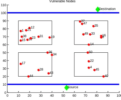
[image:6.595.335.538.213.380.2]For this scenario, number of mobility rounds for position variance of source and sink has been taken as 10. The location of source and sink is changing from one position to another after completing all iterations of Genetic Algorithm at that position. Fig 14 determines vulnerable nodes at initial position of source and sink for the scenario of 50 nodes and Fig 15 shows comparison of congestion value before and after applying genetic algorithm.
[image:6.595.330.535.436.611.2]Fig 14: Vulnerable nodes at initial position of source and sink
Fig 15: Comparison of Actual and Proposed with GA congestion value
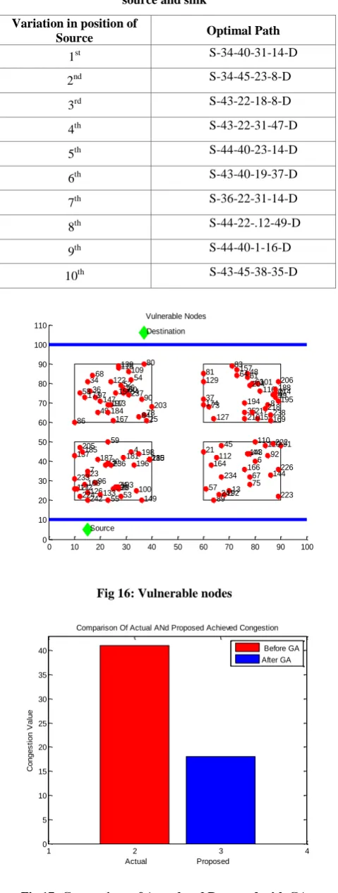
The results demonstrate the effectiveness of our algorithm in terms of congestion value. For each position variance of source and sink with respect to its initial value, optimal path is determined. Below is table representing 10 optimal paths obtained after applying genetic algorithm for each position variance of source node and sink node with respect to its initial value.
0 10 20 30 40 50 60 70 80 90 100
0 10 20 30 40 50 60 70 80 90 100 110
9 24 26 32
35 61 70 71
85 106
109
112
117 124132 140 146 153 159 182
184 196 201
222 236
246
13 21 29
37 40 51
54 56
62 73 76
87 88
110 113127
148 160
162
175 178
179 189 203214
221 231
232 238
239
245 8
23 27 30
47 48
58 64
68 97
103
114 126 137 171
188 202
207 208
216 226
228 241
25
34 39 42
44 57
65
79 89 93 96 98
108 131
135 136
141 143
152 173 190
191 194
195 197 200
206
218 229
230
234 242
247
248
Source Destination Vulnerable Nodes
1 2 3 4
0 5 10 15 20 25 30 35 40 45
Comparison Of Actual ANd Proposed Achieved Congestion
C
o
n
g
e
s
ti
o
n
V
a
lu
e
Actual Proposed
Before GA After GA
0 10 20 30 40 50 60 70 80 90 100
0 10 20 30 40 50 60 70 80 90 100 110
17 28
34 36
43 44
4 22
40 45 50 1 12
15 18 19
21 23 31
38 8
14 16 33
35 37
47
49
Source
Destination Vulnerable Nodes
1 2 3 4
0 1 2 3 4 5 6 7 8 9
Comparison Of Actual ANd Proposed Achieved Congestion
C
o
n
g
e
s
ti
o
n
V
a
lu
e
Actual Proposed
Table 4. Optimal route table for each position variance of source and sink
Variation in position of
Source Optimal Path
1st S-34-40-31-14-D
2nd S-34-45-23-8-D
3rd S-43-22-18-8-D
4th S-43-22-31-47-D
5th S-44-40-23-14-D
6th S-43-40-19-37-D
7th S-36-22-31-14-D
8th S-44-22-.12-49-D
9th S-44-40-1-16-D
10th S-43-45-38-35-D
Fig 16: Vulnerable nodes
Fig 17: Comparison of Actual and Proposed with GA congestion value
After performing simulation with 250 nodes, effectiveness of proposed algorithm is checked in terms of congestion or fitness value. Fig 16 shows vulnerable nodes and Fig 17 demonstrate comparison between actual and proposed value.
5. CONCLUSION
This paper has attempted to solve the complex and challenging issue of congestion using genetic algorithm based approach for optimal control of traffic network for different scenarios of source/and sink mobility. With every variation in position of source or sink with respect to its initial value, optimal path is found. For determining an optimal path, concept of localization regions and connection value is employed. If there are few connections between nodes, then, there is less chance of interference and less probability of congestion occurrence. Furthermore, nodes present in localized regions are assumed to be localized. A brief description of each stage of GA is presented with implementation information. Simulations are performed for different scenarios of source or/and sink mobility. Simulation results show significant improvements in terms of congestion value. The Genetic Algorithm provides excellent results even if the complexity of the network is increased by increasing the number of nodes. It has been observed that optimization results in a path with congestion or fitness value are less than actual path.
6.
FUTURE SCOPE
During the course of this work, some potential directions of future research were identified. One of the future perspectives may be achieved by incorporating packet transmission in simulation process. Significant results may be achieved by applying other optimization techniques like ant colony optimization, particle swarm optimization etc.
7.
REFERENCES
[1] J. Yick, B. Mukkherjee, D. Ghosal, “Wireless sensor network survey,”Computer Networks, Vol. 52, No. 12, pp. 2292-2330, Aug. 2008.
[2] O. Roeva, Real-World Applications of Genetic Algorithms, Publisher:InTech, ISBN 978-953-51-0146-8, 2012.
[3] M. Lyas and I. Magoub. Compact wireless and wired sensor system. CRC Press, 2004.
[4] M. Perkins, N. Correal, and B. O’Dea, “Emergent wireless sensor network limitations: a plea for advancement in core technologies,” in Proceedings of IEEE Sensors, 2002, vol. 2, pp. 1505–1509.
[5] M. N. Elshakankiri, M. N. Moustafa and Y. H. Dakroury. “Energy Efficient Routing Protocol for Wireless Sensor Networks,” in International Conference on Intelligent Sensors, Sensor Networks and Information Processing, Dec. 2008, pp. 393 – 398.
[6] G. Acs and L. Buttyabv. “A taxonomy of routing protocols for wireless sensor networks,” BUTE Telecommunication department, Jan. 2007.
[7] Arnab raha,Mrinal Kanti Naskar. “ A Genetic Algorithm Inspired Load Balancing Protocol for Congestion Controlled in Wireless Sensor Networks using Trust Based Routing Framework(GACCTR)”, Advanced Digital and Embedded Systems Laboratory, ETCE Department, Jadavpur University, Kolkata, India.
0 10 20 30 40 50 60 70 80 90 100
0 10 20 30 40 50 60 70 80 90 100 110
4 7 12 23
2428 30
53 55 59
96 100
115
121126 130 133 137
149 168
172
180 181 185
187
193 196
198 205
224 233
235 236
242
6
13 21 45 44
57 67 75 89
91 92 110 112
120 143
144 164 166
192
222
223 226 234
241 25
34 36
49 525654
58 60
68
78 80
84 86
90 97
109
113 118 122
139
147 154 156
167 173
184
197 203
237
8 35 37
48 61 63 64
73
81 83
8799 101
116
127 129
157
159169 174
188 194 195
204 206
210 214 217218238
Source
Destination Vulnerable Nodes
1 2 3 4
0 5 10 15 20 25 30 35 40
Comparison Of Actual ANd Proposed Achieved Congestion
C
o
n
g
e
s
ti
o
n
V
a
lu
e
Actual Proposed
[8] l Stojmenovic. The state of the art of sensor network. John wali and sensor.2005
[9] J. Fraden. A hand book of modern sensor: Physic, design, and application. Birkauser, 2004.
[10] Birk, W.; Osipov, E.; Eliasson, J. iRoad—Cooperative Road Infrastructure Systems for Driver Support. In
Proceedings of the 16th ITS World Congress, Stockholm, Sweden, 21–25 September 2009.
[11] Qin, H.; Li, Z.; Wang, Y.; Lu, X.; Wang, G.; Zhang, W. An Integrated Network of Roadside Sensors and Vehicles for Driving Safety: Concept, Design and Experiments. In Proceedings of the 2010 IEEE International Conference on Pervasive Computing and Communications (PerCom), Manheim, Germany, 29 March–2 April 2010.
[12] Chang, Y.; Juang, T.; Su, C.H. Wireless Sensor Network Assisted Dynamic Path Planning for Transportation Systems. In Proceedings of the 5th International Conference on Autonomic and Trusted Computing Lecture Notes Computer Science, Wuhan, China, 3–6 September 2006.
[13] Satvir Singh, Shivangna, Shelja tayal. “Analysis of Different Ranges for Wireless Sensor Node Localization using PSO and BBO and its variants”, in International Journal of Computer Applications (0975 - 8887) Volume 63 - No. 22, February 2013.
[14] Cirstea, C., Davidescu, R., & Jianu, A. (2013). Optimum communication paths for mobile WSNs using genetic algorithms. Telecommunications and Signal Processing (TSP), 2013 36th International Conference on. doi:10.1109/TSP.2013.6613940
[15] Assis, A. F., Vieira, L. F. M., Rodrigues, M. T. R., & Pappa, G. L. (2013). A genetic algorithm for the minimum cost localization problem in wireless sensor networks. Evolutionary Computation (CEC), 2013 IEEE Congress on. doi:10.1109/CEC.2013.6557650
[16] Wu, Y., & Liu, W. (2013). Routing protocol based on genetic algorithm for energy harvesting-wireless sensor
networks. Wireless Sensor Systems, IET.
doi:10.1049/iet-wss.2012.0117
[17] Basaran, C., Kang, K.-D., & Suzer, M. H. (2010). Hop-by-hop congestion control and load balancing in wireless sensor networks. Local Computer Networks (LCN), 2010
IEEE 35th Conference on.
doi:10.1109/LCN.2010.5735758
[18] Soundararajan, S., & Bhuvaneswaran, R. S. (2012). Multipath load balancing & rate based congestion control for mobile ad hoc networks (MANET). Digital Information and Communication Technology and It’s Applications (DICTAP), 2012 Second International Conference on. doi:10.1109/DICTAP.2012.6215393
[19] J. Inagaki, M. Haseyama, H. Litajima, “A genetic algorithm for determining multiple routes and its applications,” in Proceedings of the 1999 IEEE International Symposium on Circuits and Systems (ISCAS’99), pp. 137-140, Vol. 6, 1999.
[20] Y. Gao, Y. Zhuang, T. Ni, K. Yin, and T. Xue, “An improved genetic algorithm for wireless sensor networks localization.” in BIC-TA. IEEE, 2010, pp. 439–443.
[21] Damuut, L. P., & Gu, D. (2013). A Mixed Genetic Algorithm Strategy to Sensor Selection Problem in WSNs. Computational Intelligence, Communication
Systems and Networks (CICSyN), 2013 Fifth
International Conference on.
doi:10.1109/CICSYN.2013.37
[22] A. Chakraborty, S. K. Mitra and M. K. Naskar, “A Genetic Algorithm inspired Routing Protocol for Wireless Sensor Networks”, accepted in the International Journal of Computer Intelligence- Theory and Practice, number 6 Vol. 1, 2011.
[23] Y. Sankarasubramaniam, O.Akan, and I.Akyildiz, “ Event-to-sink reliable transport in wireless sensor networks”, In Proc. Of the 4th ACM Symposium on Mobile Ad Hoc Networking & Computing ( MobiHoc 2002), pages 177- 188. Annapolis, Maryland, June 2003
[24] Bavitha R and Hemalatha R, “Optimization of Path using Genetic Algorithm for Wireless Sensor Networks”,
published in the International Journal of
Communications and Engineering, Volume 05 – No.: 05, Issue 03, March 2012.
[25] Liu, B., Jiang, N., Zheng, Y., & Jing, Y. (2011). Simulation of cost optimal control of the transmission congestion management in electricity systems. Control and Decision Conference (CCDC), 2011 Chinese. doi:10.1109/CCDC.2011.5968849.
[26] M. Haenggi, D.Puccinelli, “Routing in ad hoc networks: A case for long hops,” IEEE Communications Magazine, October 2005.
[27] S. Lin, “Computer solutions of the Travelling Salesman Problem “, Bell Systems Technical Journals, Vol. 44 (1965), pp. 2245-2269.
[28] Charalambos Sergiou and Vasos Vassiliou, “Tree Forming Schemes for Overload Control in Wireless Sensor Networks”, Networks of Research Laboratory, Department of Computer Science, University of Cyprus. [29] J. Y. Potvin and J. M. Rousseau, “An exchange heuristic for routing problems with time windows”, Journal of the Operational Research Society, Vol. 46 (1995), pp. 1433-1446.
[30] Bin, L., Nan, J., Ting, L., & Yuanwei, J. (2012). Transmission congestion control research in power system based on immune genetic algorithm. Control Conference (CCC), 2012 31st Chinese