PARIS RESEARCH LABORATORY
d i g i t a l
January 1994
J ´er ˆome Barraquand
Thierry Pudet
Pricing of American
Path-Dependent
Contingent Claims
J ´er ˆome Barraquand
Thierry Pudet
The authors can be contacted at the following addresses:
J´erˆome Barraquand
Digital Equipment Corporation Paris Research Laboratory 85 Avenue Victor Hugo
92500 Rueil-Malmaison, France [email protected]
Thierry Pudet
Digital Equipment Corporation Paris Research Laboratory 85 Avenue Victor Hugo
92500 Rueil-Malmaison, France [email protected]
c
Digital Equipment Corporation 1994
We consider the problem of pricing path-dependent contingent claims. Classically, this problem can be cast into the Black-Scholes valuation framework through inclusion of the path-dependent variables into the state space. This leads to solving a degenerate advection-diffusion Partial Differential Equation (PDE). Standard Finite Difference (FD) methods are known to be inade-quate for solving such degenerate PDE. Hence, path-dependent European claims are typically priced through Monte-Carlo simulation. To date, there is no numerical method for pricing path-dependent American claims.
We first establish necessary and sufficient conditions amenable to a Lie algebraic characteriza-tion, under which degenerate diffusions can be reduced to lower-dimensional non-degenerate diffusions on a sub-manifold of the underlying asset space. We apply these results to path-dependent options. Then, we describe a new numerical technique, called Forward Shooting
Grid (FSG) method, that efficiently copes with degenerate diffusion PDE. Finally, we show
that the FSG method is unconditionally stable and convergent.
The FSG method has been implemented for a number of popular path-dependent options, and proved to be much faster than traditional Monte Carlo simulation, for a comparable accuracy. Depending on the type of option, the computation time lies between 1 and 15 seconds on a PC, for a 0:1 % precision.
The FSG method is also the first capable of dealing with the early exercise condition of American options. Furthermore, when the stock price S follows a binomial process, the method computes the exact price of any American lookback option on S. The same is true for barrier options, such as up-and-in or down-and-out options.
2 Contingent claim valuation
2 2.1 The PDE approach : : : : : : : : : : : : : : : : : : : : : : : : : : : : 32.2 The Feynman-Kac formula : : : : : : : : : : : : : : : : : : : : : : : : 3
2.3 The Black-Scholes equation : : : : : : : : : : : : : : : : : : : : : : : 3
2.4 Numerical solutions : : : : : : : : : : : : : : : : : : : : : : : : : : : : 4
3 Path dependency
53.1 A menagerie of path-dependent options : : : : : : : : : : : : : : : : : 5
3.2 An introductory example : : : : : : : : : : : : : : : : : : : : : : : : : 7
3.3 Augmenting the state space : : : : : : : : : : : : : : : : : : : : : : : 8
3.4 Degeneracy of augmented PDE : : : : : : : : : : : : : : : : : : : : : 9
4 Characterization of path-dependent price processes in two dimensions
10 4.1 The generic two-dimensional path-dependent pricing problem : : : : 114.2 Fisk-Stratonovitch stochastic differentials : : : : : : : : : : : : : : : : 12
4.3 The stochastic Frobenius integrability condition in two dimensions : : 13
4.4 Characterization of path dependent prices processes : : : : : : : : : 14
5 Characterization of path-dependent price processes: general case
15 5.1 The general diffusion problem : : : : : : : : : : : : : : : : : : : : : : 155.2 The certainty equivalence theorem of Stroock and Varadhan : : : : : 16
5.3 Frobenius integrability condition and Chow’s theory : : : : : : : : : : 17
5.4 A characterization of holonomy for degenerate diffusions : : : : : : : 19
6 The Forward Shooting Grid (FSG) method
206.1 Principle : : : : : : : : : : : : : : : : : : : : : : : : : : : : : : : : : : 21
6.2 Application : : : : : : : : : : : : : : : : : : : : : : : : : : : : : : : : : 22
6.2.1 Lookback option : : : : : : : : : : : : : : : : : : : : : : : : : : 22
6.2.2 Average-rate (Asian) option : : : : : : : : : : : : : : : : : : : : : 24
7 Convergence of the FSG method
257.1 Lipschitz conditions : : : : : : : : : : : : : : : : : : : : : : : : : : : : 25
7.2 Quantization of time : : : : : : : : : : : : : : : : : : : : : : : : : : : : 26
7.3 Quantization of space : : : : : : : : : : : : : : : : : : : : : : : : : : : 27
7.4 Convergence : : : : : : : : : : : : : : : : : : : : : : : : : : : : : : : : 27
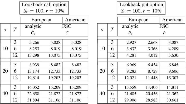
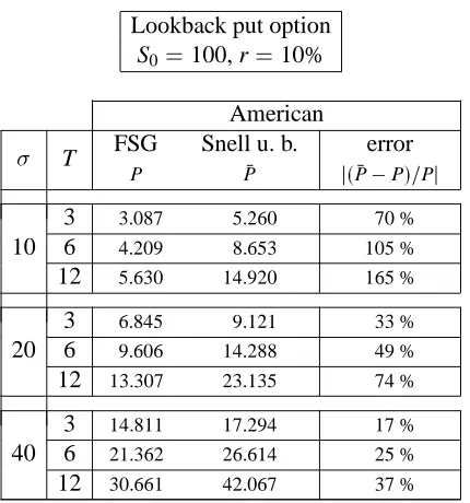
8 Results
288.1 Lookback option : : : : : : : : : : : : : : : : : : : : : : : : : : : : : : 28
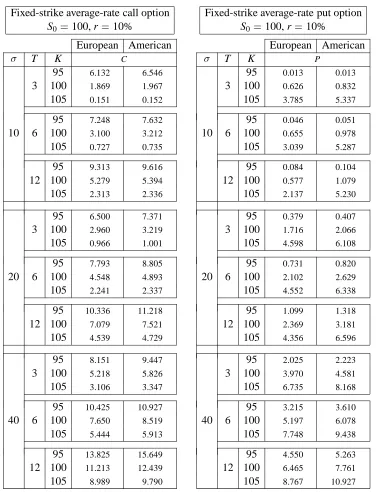
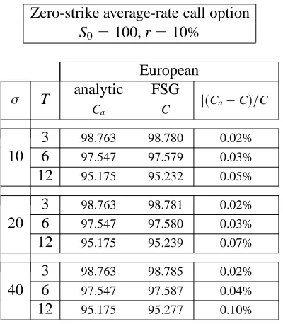
8.2 Average-rate option : : : : : : : : : : : : : : : : : : : : : : : : : : : : 30
1
Introduction
Path-dependent options are options whose payoffs depend on historical values of the underlying asset over a given time period as well as its current value. Well-known examples are lookback call (put) options, which give their owners the right to buy (sell) the asset at an exercise price equal to the minimum (maximum) price of the asset over the life of the option. Many other variants exist, e.g. capped options, barrier options etc.
Average-rate or Asian options constitute another class of path-dependent instruments, whose payoffs depend on the arithmetic average value of the asset price for some time period. Popular examples include fixed-strike, and floating-strike average-rate options.
Since their introduction in 1982, path-dependent options found their way in several places such as common stocks and foreign exchange markets, by meeting specific risk management and investment needs. As evidence of their increasing popularity, some instruments such as capped options have recently begun to be traded on the Chicago Board of Options Exchange and American Stock Exchange, see e.g. Hunter and Stowe (1992).
The modern approach to path-dependent option pricing relies on the dynamic hedging principle of the Black-Scholes model (Black and Scholes (1973)). In their seminal work, Goldman et al. (1979) have shown that a hedge portfolio could be constructed for an option to buy at the historical maximum, and that closed-form valuation formulas exist in the European case. Garman (1989) developed another valuation model, which separates the lookback option into two underlying options, and gives furthermore the ability to price a European option on an asset that pays dividends. The Asian option is analyzed by Yor (1989). Conze and Viswanathan (1991) derive explicit valuation formulas of most European barrier options, as well as some upper bounds in the American case. Kemna and Vorst (1990) use Monte Carlo simulation with a specific variance reduction method to compute the price of fixed-strike average-rate options.
The path-dependent pricing problem can be cast into the classical Black-Scholes valuation framework through inclusion of the path dependent variables into the state space (see e.g. Stanton (1989)). In a few simple cases, the resulting augmented PDE admits a closed form solution. However, the use of numerical techniques is mandatory in most practical situations. The augmented PDE associated with a path-dependent problem is generally degenerate, i.e. the instantaneous covariance matrix is singular. Finite Difference (FD) methods are numer-ically stable, but they introduce a spurious additional numerical diffusion, and therefore do not converge towards the theoretical solution. The only practical technique to date consists in computing the price through Monte Carlo simulation by means of the Feynman-Kac represen-tation. This approach is satisfactory for pricing European path-dependent contingent claims. However, it cannot deal with the early exercise conditions of American claims.
be used, and the memory required to conduct the integration.
For this purpose, we use the concept of symmetric multiplication for stochastic integrals, which leads to the notion of Fisk-Stratonovitch differential. Then, we use standard results regarding discrete approximations of multidimensional diffusion processes that establish a link between stochastic differential equations and deterministic optimal control theory. Finally, we use standard results on the accessibility of deterministic control systems. This leads to a Lie algebraic characterization of holonomic PDE.
Then, we apply these results to popular types of path-dependent pricing problems. We show in particular that the average-rate option pricing PDE is non-holonomic. Finally, we present a new numerical technique, called Forward Shooting Grid method, that efficiently copes with the degeneracy of these non-holonomic PDE. In particular, we show that, unlike FD methods, the FSG method is unconditionally stable and convergent in the presence of arbitrary degeneracies.
The FSG method has been implemented, and demonstrated the following capabilities:
1) It is much faster than traditional Monte Carlo simulation, for a comparable accuracy.
Depending on the type of option, the computation time on a PC lies between 1 and 15 seconds, for a 0:1% precision.
2) It can deal with the early exercise condition of American options. To the best of our
knowledge, this is the first method capable of pricing American path-dependent options.
3) When the stock price S follows a Cox-Ross-Rubinstein binomial process, the method
computes exactly the price of any (e.g. minimum or maximum) American lookback option on S. This is also true for barrier options, such as up-and-in or down-and-out options.
The next section briefly reviews the basic ingredients of the modern contingent claim valuation model, and discusses the alternative implementations of the numerical solutions. Section 3 examines how path dependency can be alleviated through state augmentation, allowing for path-dependent claims to be priced in the standard valuation framework. It also emphasizes the difficulty of solving the resulting degenerate equations with standard finite difference methods. Sections 4 and 5 establish necessary and sufficient conditions of holonomy for degenerate dif-fusions. Section 6 introduces the Forward Shooting Grid method which efficiently copes with this degeneracy, as well as with the early exercise condition of American path-dependent secu-rities. Section 7 establishes the convergence of the FSG method for general multidimensional diffusion processes. Finally, Section 8 gives several examples of European and American prices for various path-dependent options, and discusses the results.
2
Contingent claim valuation
implementations of the numerical solutions.
2.1 The PDE approach
There exists an asset-price stochastic process St governing the evolution of the state variable S, which follows the It ˆo’s stochastic differential equation (SDE):
dSt = m(t;St)dt+b(t;St)dw; S0>0; (2.1)
where w is a standard Brownian motion.
There also exists a bond-price process Bt, governed by the SDE:
dBt = r(t;St)Bt;B0 >0:
This process models the continuously compounding risk-free interest rate.
Consider a derivative security with terminal payoff g(ST), where g is some continuous real
function that depends on state variable S. It is shown that in the absence of arbitrage, the price
C(t;St)of the derivative security at time t solves the partial differential equation (PDE):
r(t;S)C(t;S)+ @C
@t
(t;S)+r(t;S)S @C @S
(t;S)+
1 2b
(t;S)
2 @
2C
@S
2(t;S)=0 (2.2)
with the boundary condition C(T;S)=g(S).
2.2 The Feynman-Kac formula
Under suitable technical conditions for functions r,, and g, the Feynman-Kac (FK) formula
gives the solution to eq. (2.2):
C(t;S) = Et
exp
Z
T
t
r(u;ˆSu)du
g(ˆST)
; (2.3)
where ˆSuis the It ˆo process defined by:
ˆSu = St; ut
d ˆSu = r(u;ˆSu)ˆSudu+b(u;ˆSu)dw; ut:
Therefore, the value (price) C(t;S)of a derivative security can be interpreted as the expectation
of its discounted payoff under the modified (aka risk-neutral) process ˆSu, whose expected rate of return is the riskless interest rate of the market.
2.3 The Black-Scholes equation
In the Black-Scholes model, the stock price S follows a log-normal process, with r and
constant:
dSt = Stdt+Stdw; S0>0 dBt = rBt; B0>0:
In this case, eq. (2.2) reduces to the Black-Scholes equation:
r C(t;S)+ @C
@t
(t;S)+r S @C @S
(t;S)+
1 2
2S2 @
2C
@S
2(t;S)=0; (2.4)
with boundary condition C(T;S)=g(S)=max(0;S K).
The change of variable
Z = log(S=S0) t; =r
2
=2; (2.5)
simplifies eq. (2.4) into:
rC+ @C
@t +
1 2
2@
2C
@Z
2 =0; (2.6)
with the boundary condition C(T;Z)=max(0;S0e
Z+(T t) K).
Looking for a solution of the form C(t;Z)=e
r(T t)
E(t;Z), eq. (2.6) reduces to the (backward)
heat equation:
@E @t
1 2
2@
2E
@Z
2 = 0; (2.7)
with the boundary condition E(T;Z)=e
r(T t)
max(0;S0e
Z+(T t) K).
Eq. (2.7) admits for solution the Black-Scholes option pricing formula:
C(t;S) = SΦ(X) e
r(T t)
KΦ(X p
T t)
X =
1
p
T t log
(S=K)+(+
2
)(T t)
;
whereΦis the cumulative standard normal distribution function.
2.4 Numerical solutions
Monte Carlo simulation.
The space complexity (memory requirement) is linear in the number of state
vari-ables. In general, the time complexity (computation time) is quadratic in the number of state variables.
Due to the high number of samples usually required to get sufficient precision,
execution times are significantly greater than those of finite difference methods.
The early exercise condition of American options cannot be dealt with.
PDE integration. In the context of asset pricing problems, PDEs usually reduce to simple
advection-diffusion equations, whose solutions are most simply computed through finite difference methods.
Both the time and space complexities of FD methods grow exponentially in the
number of state variables. This makes the PDE approach attractive only when the number of underlying assets is small.
Numerical instabilities of FD methods can be a delicate issue. In particular, it is
well-known that FD methods are ill suited to solving degenerate PDEs, that is PDEs for which the covariance matrix is singular.
In general, FD implementations run significantly faster than corresponding Monte
Carlo simulations.
PDE solving methods are the only ones that easily handle the early exercise
condi-tion of American opcondi-tions1.
3
Path dependency
This section first examines popular examples of path dependent problems, then describes how path dependency can be alleviated through state augmentation. It also emphasizes the difficulty of solving the resulting PDEs with standard FD methods.
3.1 A menagerie of path-dependent options
Historically, many similar path-dependent options have been given different names. This section presents the most popular path-dependent options, giving explicit formulas for their associated payoffs.
Without loss of generality, we will assume all options to be issued at initial time t=0, expiring
at time T > 0. We will write ST the value of asset S at expiration time T, and K the strike
or exercise price of the option. CT (resp. PT) will denote the payoff of a call (resp. put) at expiration time, and C (resp. P) the sought value of the call (resp. put) at initial time.
1The existence of solutions to advection diffusion PDE with early exercise boundary conditions has been studied
Let Mt(resp. mt) be the maximum (resp. minimum) value of asset S over the time period [0;t]:
Mt = max0 tS mt = min0
tS :
(3.1)
Let also Atbe the value of the arithmetic average of S over [0;t]:
At =
1
t Z
t
0
Sd (3.2)
Ordinary option. An ordinary call (resp. put) option gives its owner the right to buy (resp.
sell) S at strike K:
CT = max(0;ST K) PT = max(0;K ST):
Lookback. A lookback call (resp. put) gives its owner the right to buy (resp. sell) S at its
lowest (resp. greatest) price over time period [0;T]:
CT = ST mT PT = MT ST:
Option on extrema. A call (resp. put) on maximum (resp. minimum) is like an ordinary
option, but the spot is to be replaced with the historical maximum (resp. minimum) value of S:
CT = max(0;MT K) PT = min(0;K mT):
Capped options. A capped call (resp. put) option is like an ordinary option, as long as the
historical maximum (resp. minimum) of S stays below (resp. above) a predefined upper (resp. lower) barrier price b. Should the maximum (resp. minimum) reach (resp. fall below) that barrier, the option is automatically exercised.
CT =
b K if MT b
max(0;ST K) otherwise
PT =
K b if mT b
max(0;K ST) otherwise:
Barrier options. Barrier options are also known as knock-out, knock-in, or trigger options.
Down-and-out call. Up-and-out put.
A down-and-out call (resp. up-and-out put) behaves like an ordinary call (resp. put) as long as the historical minimum (resp. maximum) of S stays above (resp. below) a predefined lower (resp. upper) barrier price b. Should the minimum (resp. maximum) reach or fall below (resp. reach or rise above) that barrier, the payoff becomes zero:
CT =
max(0;ST K) if mT >b
0 otherwise
PT =
max(0;K ST) if MT <b
0 otherwise:
Down-and-in call. Up-and-in put.
A down-and-in call (resp. up-and-in put) behaves like an ordinary call (resp. put) as long as the historical maximum (resp. minimum) of S stays below (resp. above) a predefined barrier upper price b. Should the maximum (resp. minimum) reach or rise above (resp. reach or fall below) that barrier, the payoff becomes zero:
CT =
max(0;ST K) if MT <b
0 otherwise
PT =
max(0;K ST) if mT >b
0 otherwise
Average-rate options. Average-rate options are also known as Asian options. Their payoffs
depend on the value of the arithmetic average of S over a given time period. There are two types of such options: fixed-strike, and floating-strike.
A fixed-strike average-rate option is like an ordinary option, with the time average ATsubstituted for ST:
CT = max(0;AT K) PT = max(0;K AT):
Symmetrically, in the payoff of a floating-strike average-rate option, the time
average AT is substituted for the strike K:
CT = max(0;ST AT) PT = max(0;AT ST):
3.2 An introductory example
only of the current value of asset S, i.e. C = C(St;t). If this is not the case, the security is
termed path-dependent. To understand the implications of such path-dependency with respect to the PDE solving approach, the following sections draw on an example developed in Stanton (1989) for the valuation of a simplified zero-strike Asian option in the Black-Scholes model.
Consider a stock S with no dividends, which follows a log-normal price process. Also, assume a constant risk-free interest rate. An option on S is issued at time t=0, expiring at time T >0,
whose terminal payoff gTis the arithmetic average ATof S over period [0;T], cf. eq. (3.2).
Applying the Feynman-Kac formula, the arbitrage-free price of this option can be computed as the discounted expectation of its payoff under the risk-neutral process ˆSu:
ˆSu = St; ut
d ˆSu = r ˆSudu+ˆSudw; ut;
and
C(t) =
1
Te
r(T t) Et
Z
T
0
ˆSudu
=
1
Te
r(T t) Z T 0 Et ˆSu du:
By definition of ˆSu, Et
ˆ
Su
= St for u t. For u t, ˆSu is a log-normal process, whose
expectation at time t is given by:
Et
ˆSu
= Ste
r(u t) : Therefore, Z T 0 Et ˆSu du = Z t 0 Et ˆSu du+ Z T t Et ˆSu du = Z t 0
Sudu+ St
r
er(T t)
1
:
Finally,
C(t) = C(t;St;At)
=
e r(T t) T
Z
t
0
Sudu+ St
rT
1 e r(T t)
;
(3.3)
which clearly shows that the value of the security, as well as its payoff are path-dependent.
3.3 Augmenting the state space
Let us therefore incorporate A as the second state variable. Atbeing the average value of S over period [0;t], t T, with A0=S0, the law of evolution of Atis obtained by differentiating eq.
(3.2):
dAt=
1
t(St At)dt: (3.4)
The value of the option at time t becomes C=C(S;A;t). Using the same arbitrage arguments
as in the regular case, it is shown that in absence of arbitrage, Atsolves the PDE:
rC+ @C
@t +rS
@C @S
+
1 2
2S2@
2C
@S
2 +
1
t
(S A) @C @A
=0; (3.5)
with the boundary condition C(T;S;A)=g=A.
Eq. (3.5) is in fact the Black-Scholes equation (2.4), into which the term 1=t(St At) @C @A
has been incorporated. By augmenting the state space, the value of the option only depends on the current values of the state variables S and A, hence path dependency has been alleviated. Furthermore, for this particular boundary condition, a closed-form formula for C(t;St;At)is
easily found:
C(t;St;At) =
e r(T t) T tAt+
St
rT
1 e r(T t)
; (3.6)
which is exactly eq. (3.3) above.
In the case of a fixed-strike Asian option with a more realistic terminal payoff g=max(0;A K), eq. (3.5) is still valid but the new boundary condition makes it impossible to find a
closed-form closed-formula for the price. In general, only numerical methods can handle path-dependent asset pricing problems, with the usual alternative of Monte Carlo simulation vs. PDE solving.
3.4 Degeneracy of augmented PDE
Augmented PDE are degenerate in nature. Intuitively, the degeneracy comes from the fact that the augmented state variables, such as At and St, are correlated. In other words, the increments dSt and dAt of asset price and time average are not independent, which implies that the deterministic relationship between them, as expressed in eq. (3.5) cannot be readily integrated. In practice, any numerical scheme that approximates an augmented PDE, although it can be made stable, will not necessarily converge to a solution. This makes the standard FD approach impractical. Again, we shall illustrate this with the example of the zero-strike Asian option, eq. (3.6) providing analytic solutions for reference.
In eq. (3.5), a discontinuity occurs at t =0, which can be eliminated by the change of variable Y =tA. Together with the change indicated in eq. (2.5), they simplify eq. (3.5) into:
@E @t
+
1 2
2@
2E
@Z
2 +S
@E @Y
with the boundary condition E(T;Z;Y)=e
rTY
=T.
Because there is no second-order term in Y, eq. (3.7) is a strongly degenerate two-dimensional advection-diffusion PDE. invert a singular matrix. Writing E(t;Z;Y)as E
n j;k
= E(tn;Z
n j;Y
n k),
eq. (3.7) is approximated with the following explicit scheme:
Dt(t) =
1 2
2D
11(t+∆t)+S(t+∆t)D2(t+∆t);
where
Dt(t) = En
j;k
En+1
j;k
∆t
= @ @t
E+O(∆t)
D2(t) =
Enj;k+1 E
n j;k 1
2∆Y
= @ @Y
E+O(∆Y
2
)
D11(t) = Enj
+1;k
2Enj
;k +E
n j 1;k
∆Z2 =
@
2
@Z
2E+O(∆Z
2
):
Eq. (3.7) is then backward integrated as follows:
uZ =
2∆t
∆Z2
uY = S
n+1
j ∆t
∆Y; Ejn
;k
= (1 uZ)E
n+1
j;k +
1
2uZ(E
n+1
j+1;k +E
n+1
j 1;k )+
1
2uY(E
n+1
j;k+1
En+1
j;k 1 ) n = N 1;:::;0
j = n;:::;n k = 0;:::;km
(3.8)
with the boundary condition
ENj ;k
= e
rTYN k =T j = N;:::;N k = 0;:::;km:
We implemented the scheme (3.8), and compared results with those obtained with formula (3.6). Not surprisingly, the numerical procedure failed to give accurate results on a broad range of input parametersand r.
4
Characterization of path-dependent price processes in two dimensions
We establish necessary and sufficient conditions under which degenerate diffusion PDE can be reduced to lower-dimensional non-degenerate PDE on a sub-manifold of the state space. A degenerate PDE that can be reduced in such a way is called holonomic. It is called
non-holonomic otherwise. It is important to determine whether a given PDE is non-holonomic or not,
since this property influences both the type of numerical integration technique that can be used, and the memory required to conduct the integration. We introduce in this section the main intuition behind this characterization in the two dimensional case. In the next section, we treat the general case.
4.1 The generic two-dimensional path-dependent pricing problem
We consider a price process St following the It ˆo SDE (2.1), and an arbitrary path-dependent variable At:
At =Ψ [S ]
t
We assume that At follows an It ˆo SDE of the type:
dAt =mA(t;St;At)dt+bA(t;St;At)dw
For example, if At is the mean value of Stup to time t, we see from the previous section that:
mA(t;S;A)=
1
t(S A); bA(t;S;A)=0
In order to compute the price of a path-dependent contingent claim C(t;St;At), we must solve
for the following two-dimensional degenerate PDE:
rC+ @C
@t +mS
@C @S
+
1 2b
2
S
@
2C
@S
2 +mA
@C @A
+
1 2b
2
A
@
2C
@A
2 +bSbA
@
2C
@S@A
=0 (4.1)
where: mS =rS; bS =b.
The numerical integration of the above equation requires a priori to quantize both variables S and A. Hence, if each variable is quantized using N samples, the memory requirement of the numerical pricing procedure is proportional to N2.
However, since the time evolutions of S and A depend on the same Brownian motion W, there is a simple relationship between the three (stochastic) differentials dt, dS, and dA:
d!=(mSbA bSmA)dt bAdS+bSdA=0 (4.2)
The numerical integration of the PDE will require a memory proportional to N2 only if this differential relationship cannot be integrated, i.e. if there is no potential function F(t;S;A)and
no integrating factor(t;S;A)such that:
Indeed, if such F and exist, then the differential relationship (4.2) is equivalent to the
following:
F(t;St;At)=F(0;S0;A0)
Hence, we can perform (under suitable technical conditions) the following change of variables in PDE (4.1):
= Φt(t;S;A) = t
Σ = ΦS(t;S;A) = S
F = ΦF(t;S;A) = F(t;S;A)
and get:
rC+ @C @
+mS @C @Σ + 1 2b 2 S @ 2C @Σ
2 +mF
@C @F + 1 2b 2 F @ 2C @F
2 +bSbF
@
2C
@Σ@F
=0 (4.3)
where we have defined for notational convenience:
mF = @F
@t +mS
@F @S + 1 2b 2 S @ 2F @S
2 +mA
@F @A + 1 2b 2 A @ 2F @A
2+bSbA
@
2F
@S@A
and
bF =bS @F @S
+bA @F @A
But by It ˆo’s formula:
dF=mFdt+bFdw
Since by assumption dF=d! =0, we get mF =bF =0. Hence, the transformed PDE (4.3)
simplifies to the usual one-dimensional Black-Scholes equation:
rC+ @C @
+mS @C @Σ + 1 2b 2 S @ 2C @Σ
2 =0 (4.4)
In order to price a contingent claim with terminal payoff g(ST;AT), one must first solve for A = (t;S) as a function of t and S in equation F(t;St;At) = F(0;S0;A0), and then solve
backwards in time the above one-dimensional PDE with the boundary condition C(T;S;A)= g(S;(T;S)). The memory required to conduct the numerical integration is now proportional
to N instead of N2. Also, the above one dimensional PDE is not degenerate, and can be
integrated using standard FD methods.
4.2 Fisk-Stratonovitch stochastic differentials
It is an important matter to characterize the conditions under which the differential relationship (4.2) can be integrated. For that purpose, we will first introduce the notion of stochastic differential in the Fisk-Stratonovich sense.
Let 0=t0 < t1 < :::<tm =t be an arbitrary partition of the interval[0;t]with a modulus =maxi(ti
Formally, the Fisk-Stratonovitch SDE dx =bdw for two continuous semi-martingales b;w
can be interpreted as a notation for the identity
8t; x(t)=x(0)+ lim !0
m 1
X
j=0
b(tj)+b(tj +1
)
2 (w(tj +1
) w(tj))
where the limit is taken in probability.
Intuitively, whereas the It ˆo differential dx=bdw is a forward differential which can be loosely
interpreted as:
x(t+dt)=x(t)+b(t)(w(t+dt) w(t))
the Fisk-Stratonovitch differential dx=bdw is a symmetric differential, which can be loosely
interpreted as:
x(t+dt)=x(t)+
b(t)+b(t+dt)
2
(w(t+dt) w(t))
It can be shown (see e.g. Karatzas and Shreve (1988)) that, unlike It ˆo differentials which follow It ˆo’s chain rule, Fisk-Stratonovitch differentials follows the chain rule of the classical differential calculus. In particular, for any smooth real-valued function f(t;x1;:::;xd) and
continuous vectors of semi-martingales X=(x1;:::;xd), we have: df(t;X)=
@f @t
(t;X)dt+
d
X
i=1 @f @xi
(t;X)dxi
Finally, it can be shown that there is the following relationship between It ˆo and Fisk-Stratonovitch SDE. If X =(x1;:::;xd)follows the It ˆo SDE:
8i2[1;d]; dxi =mi(t;X)dt+
k
X
j=1
bij(t;X)dwj
Then
8i2[1;d]; dxi = 0 @m
i 1 2
d
X
l=1
k
X
j=1 blj
@bij @xl
1 Adt
+
k
X
j=1
bijdwj
4.3 The stochastic Frobenius integrability condition in two dimensions
In this subsection, we introduce the integrability conditions for equation (4.2). We consider for simplicity the case d =2, k=1. The system of It ˆo SDE:
dx1=m1(t;x1;x2)dt+b1(t;x1;x2)dw dx2=m2(t;x1;x2)dt+b2(t;x1;x2)dw
admits the following Fisk-Stratonovitch equivalent:
with
˜
m1 =m1
1 2
b1
@b1 @x1
+b2 @b1 @x2
˜
m2 =m2
1 2
b1
@b2 @x1
+b2 @b2 @x2
By eliminating dw, we get the following differential relationship:
d!=!0dt+!1dx1+!2dx2=(m˜1b2 m˜2b1)dt b2dx1+b1dx2 =0
By the Fisk-Stratonovitch (i.e. classical) chain rule, a sufficient condition for the existence of a potential function F(t;x1;x2)and an integrating factor(t;x1;x2)such that dF =d!is:
@F @t
=!0; @F @x1
=!1; @F @x2
=!2 (4.5)
From the above relations and the symmetry of the second order mixed partial derivatives of F, we get after elimination of:
!0
@!2 @x1
@!1 @x2
+!1
@!2
@t
@!0 @x2
+!2
@!1
@t
@!0 @x1
=0 (4.6)
It can be shown (see section 5) that the above relation is a necessary and sufficient condition for the existence of F. We can express the above condition in terms of miand bjinstead of!i. Let
us denote B0 =(1;m˜1;m˜2)
Tand B
1=(0;b1;b2)
T. After elementary algebraic manipulations,
the integrability condition (4.6) is shown to be equivalent to:
det B0;B1;[B0;B1]
=0
where[B0;B1]is the Lie Bracket (see also section 5) of the vector fields B0 and B1, i.e. the
vector field:
[B0;B1]=dB0:B1 dB1:B0
and where dBidenote the Jacobian matrix of the vector field Bi.
4.4 Characterization of path dependent prices processes
We consider the path-dependent price process of subsection (4.1). We take x1=S and x2=A.
Define
˜
mS=mS
1 2bS
@bS @S
˜
mA=mA
1 2
bS
@bA @S
+bA @bA
@A
and let B0 =(1;m˜S;m˜A)
T, and B
1=(0;bS;bA)
T. Then:
The degenerate two-dimensional Black-Scholes PDE (4.1) in the variables (S,A) can be reduced to the one-dimensional non-degenerate PDE (4.4) if and only if the following condition is satisfied:
det B0;B1;[B0;B1]
We can apply the above result to the case of a path-dependent variable A which is instantaneously riskless. i.e. bA =0.
We have: B0=(1;m˜S;m˜A)
T, B
1 =(0;bS;0)
T, hence
det B0;B1;[B0;B1]
= b
2
s
@mA @S
Therefore, the problem can be reduced to a one-dimensional problem iff mAdoes not depend on S. This is obviously not the case for the average-rate option pricing problem:
@mA @S
=
1
t 6=0
We can state:
The average-rate option pricing PDE (3.5) cannot be reduced to a one-dimensional non-degenerate PDE.
5
Characterization of path-dependent price processes: general case
In this section, we turn to a generalization of the above result.
5.1 The general diffusion problem
We consider an advection-diffusion equation of the type:
@f @t
= rf +
d
X
i=1 mi
@f @xi
+
1 2
X
i;j ij
@
2f
@xi@xj
(5.1)
where X =(x1;:::;xd)
T
2R
d, M
=(m1;:::;md)
T, with the following boundary condition:
f(T;x1;:::;xd)=g(x1;:::;xd)
We assume that the real valued functions r(t;x1;:::;xd) >0, mi(t;x1;:::;xd);i2[1;d], and ij(t;x1;:::;xd);(i;j)2[1;d]
2on
[0;1[R
dare bounded and sufficiently smooth. We assume
furthermore that for any t;x1;:::;xdthe matrix:
Γ(t;x1;:::;xd)=(ij(t;x1;:::;xd))
(i;j)2[1;d]
2
is symmetric and non-negative. We denote by B its Cholesky decomposition:
Γ=BB
T
By the Feynman-Kac formula, the solution of the above PDE can be expressed:
f(t;x1;:::;xd)=Et
exp
Z
T
0
r(;X())d
g(X(T))
where X is the solution of the SDE:
dX =Mdt+BdW; X(t)=(x1;:::;xd)
T (5.2)
W=(w1;:::;wk)is a k-dimensional standard Brownian motion.
We can define the vector ˜M:
8i2[1;d]; m˜i =mi
1 2
d
X
l=1
k
X
j=1 blj
@bij @xl
Then, from subsection (4.2):
dX=Mdt˜ +BdW (5.3)
We denote by SW(X0)the support of the above SDE for X(0)=X0, i.e. the smallest closed set
of paths X(t)(elements of the Wiener space Karatzas and Shreve (1988); Ikeda and Watanabe
(1981)) such that Prob(S
W
(X0)) = 1. The set of accessible states at time t of SDE (5.3) for X(0)=X0, i.e. the set of values X(t)for elements of S
W
(X0), is denoted by A
W
(t;X0). In other
words, AW(t;X0)is the time t projection of S
W
(X0). Clearly,
Prob(X(t)2A
W
(t;X0))=1
The set of accessible states from X0for system (5.3) is defined as:
AW(X0)=[t 0A
W
(t;X0)
Clearly,
Prob(8t;X(t)2A
W
(X0))=1
5.2 The certainty equivalence theorem of Stroock and Varadhan
The following theorem was first established by Stroock and Varadhan (1972). We use here the formulation of Ikeda and Watanabe, where the theorem is established as a consequence of general convergence results for approximations of diffusion processes (see Ikeda and Watanabe (1981)).
We consider the deterministic control system:
dX
dt =M˜ +B dU
dt (5.4)
We define the support SU(X0) of system (5.4) as the set of all possible paths X(t)starting at X0for all possible control paths U. Similarly, we define the set AU(t;X0)R
dof accessible
states at time t from X0 as the set of states X
2 R
d such that there exist a control U
(t)
verifying X
= X(t). The set A
U
(X0) R
d of accessible states from X
0 is similarly defined
as AU
(X0) = [t 0A
U
(t;X0). Finally, we say that a state X
is weakly accessible from X0
if there exist a sequence X0;X1;:::;Xn =X
such that either Xi+1 is accessible from Xi, or Xi is accessible from Xi+1. The set of states weakly accessible from X0 is denoted WA
(X0).
By definition, any accessible state is weakly accessible, i.e. A(X0) WA(X0). For a
non-symmetric system, i.e. a system such that the controls U cannot always be inverted, then there may be weakly accessible states that are not accessible.
We have the following fundamental result (Stroock and Varadhan (1972)):
(Stroock and Varadhan, 1972)
For any X0, the support of the Fisk-Stratonovitch system (5.3) is the closure of
support of the deterministic system (5.4):
SW(X0)=S
U
(X0)
We will only use the following immediate corollary:
For any X0, and any time t, the set of accessible states at time t from X0 of the
Fisk-Stratonovitch system (5.3) is the closure of the set of accessible states at time t from X0of the deterministic system (5.4):
8t0; 8X0; A
W
(t;X0)=A
U
(t;X0)
5.3 Frobenius integrability condition and Chow’s theory
In the previous section, we used the certainty equivalence theorem in order to establish a link between stochastic and deterministic accessibility for differential equations. In this section, we apply standard result on the accessibility of deterministic control systems to characterize the integrability of degenerate SDE.
We consider again the deterministic system (5.4). For the purpose of the following discussion, we will include the time variable t in the state, i.e. we consider the state of the system at time t to be Y =(y0(t);y1(t);:::;yd(t))=(t;x1(t);:::;xd(t))2R
d+1
. If bijdenote the elements of the matrix B, we define the extended(d+1)(d+1)matrix ˜B:
˜ B= 0 B B B B B B @
1 0 ::: 0
˜
m1 b11 ::: b1d
: : :
: : :
: : :
˜
Then, system (5.4) is equivalent to the following system in Rd+1
:
dY dt =B˜
d ˜U
dt (5.5)
where ˜U(t) = (t;U(t)) = (t;u1(t);:::;uk(t)) = (˜u0(t);˜u1(t);:::;˜uk(t)) is the extended
control.
Let AU˜(Y0)denote the set of extended states accessible from Y0 =(0;X0). Clearly: AU˜(Y0)=[t
0
ftgA
U
(t;X0)
and
WAU˜(Y0)=[t 0
ftgWA
U
(t;X0)
By definition, any accessible state is weakly accessible. Reciprocally, if the drift is zero, i.e. ˜
M = (m˜1;:::;m˜d) = 0, then weak accessibility is equivalent to accessibility. Indeed, since
the system (5.5) is symmetric in the control variable U (i.e. U is an admissible control iff U
is an admissible control), the extended control ˜U becomes symmetric for a zero drift.
If ˜M=0, we get:
8t; WA
U
(t;Y0)=A
U
(t;X0)
We now recall the definition of the Lie bracket of two vector fields. Let(V
1
;V
2
) be any pair
of vector fields in Rd+1
.
Given any point Y0 = (t;X0) 2 R
d+1
, let us consider a path starting at Y0 and obtained by
concatenating the four following paths:
- the first path follows the flow2of V1duringt;
- the second path follows the flow of V2duringt;
- the third path follows the flow of V1duringt;
- the fourth path follows the flow of V2duringt.
Let Y1=(t+t;X1)be the configuration reached at the end of these four paths. A
straightfor-ward Taylor expansion shows that:
lim
t!0
Y1 Y0
t
2 =dV
2
V
1 dV1
V
2
;
where dV2V
1and dV1
V
2denote the products of the
(d+1)(d+1)Jacobian matrices:
2
The integral curve of a vector field V is a curve whose tangent at every point Y is V(Y). We say that the curve
dV2 = 0 B B B B B @ @v 2 0
@y0 :::
@v
2 0
@yd
: : : : : : @v 2 d
@y0 :::
@v
2
d
@yd 1 C C C C C A
; dV1
= 0 B B B B B @ @v 1 0
@y0 :::
@v
1 0
@yd
: : : : : : @v 1 d
@y0 :::
@v
1
d
@yd 1 C C C C C A ;
and the(d+1)-vectors:
V1=(v
1
0;v
1
1 ::: v
1
d)
T; V2
=(v
2
0 v21 ::: v
2
d)
T
:
The expression dV2V
1 dV1
V
2determines a new vector field which is commonly denoted
by[V
1
;V
2
]and called the Lie bracket of V
1and V2.
Let B0;:::;Bdbe the columns of the extended matrix ˜B. By definition, the Control Lie Algebra
associated with system (5.5), denoted by CLA(B˜), is the smallest Lie algebra which contains B0;:::;Bd. Stated otherwise, CLA(B˜) is the subspace of vector fields generated by all the
linear combinations of vector fields B0;:::;Bdand all their Lie brackets recursively computed.
For every Y0 2R
d+1
, let CLA(B˜)(Y0) denote the subspace of vectors spanned by the vector
fields of CLA(B˜) at Y0. A connected sub-manifold Mof R
d+1
is an integral sub-manifold of CLA(B˜)if at each Y 2R
d+1
the tangent space toMis contained in CLA(B˜)(Y). Mis a maximal integral sub-manifold of CLA(B˜)if it is not properly included in any other integral
manifold.
The Frobenius integrability theorem can be stated as follows:
Frobenius Integrability Theorem If the dimension of CLA(B˜)(Y)has a constant value r for every Y 2R
d+1
, there exists a partition of Rd+1
into maximal integral sub-manifolds of CLA(B˜)all of dimension r.
The maximal integral sub-manifold of dimension r passing through Y is denotedMr(Y).
The following results derive from the work of Chow (1939). They were elucidated in Hermann (1963); Haynes and Hermes (1970); Lobry (1970); Sussmann and Jurdjevic (1972); Hermann and Krener (1977). We follow the presentation of Hermann and Krener (1977).
Chow’s Theorem If the dimension of CLA(B˜)(Y)has a constant value r for every Y 2R
d+1 , then
8Y 2R
d+1
; Mr(Y)=WA
U
(Y) Furthermore, the interior of AU(Y)as a subset ofMr(Y)=WA
U
5.4 A characterization of holonomy for degenerate diffusions
By inspection of the extended matrix ˜B, and since the original matrix B is by definition regular,
the minimal dimension of the Control Lie Algebra is rmin=k+1.
Let us assume that the Control Lie Algebra has a constant dimension k+1 r d+1.
We will show that there exist exactly m=d+1 r constraints satisfied almost surely by the
solution of the Fisk-Stratonovitch system (5.3).
We will first show m d+1 r. Indeed, Chow’s Theorem states that the set of weakly
accessible states for (5.5) is a sub-manifold of dimension r. This means that there exist a set of
d+1 r independent constraints F= F1(t;x1;:::;xd);:::;Fd +1 r
(t;x1;:::;xd)
such that
8t2R; 8X02R
d
; WA
U
(t;X0)=fX2R
d
; F(t;X)=F(0;X0)g
This result, together with the Certainty Equivalence Theorem, implies that the set of accessible states from X0of the Fisk-Stratonovitch system (5.3) satisfies the constraints F(t;X)=F(0;X0)
almost surely. Indeed, the set of accessible states is a subset of the set of weakly accessible states. Hence md+1 r.
Reciprocally, let us assume that the solution X(t)of the Fisk-Stratonovitch system (5.3) satisfies
almost surely m independent constraints F = (F1;:::;Fm). By the certainty equivalence
theorem, we have F(A
˜
U
(Y0)) = F(Y0). But, by Chow’s theorem, the interior of A
˜
U
(Y0)in Mr is not empty. Hence, it cannot satisfy more than d+1 r constraints, since Mr is of
dimension r. This implies md+1 r.
We can state:
Condition for the existence of d+1 r constraints
If the Control Lie Algebra CLA(B˜) has constant dimension r, then there exist
exactly d+1 r independent constraints F = (F1;:::;Fd +1 r
) such that the solution of the Fisk Stratonovitch system (5.3) satisfies the constraints almost surely.
Prob 8t;F(t;X(t))=F(0;X0)
=1
A degenerate It ˆo SDE of the form (5.2) and a degenerate advection-diffusion PDE on the form (5.1) are called holonomic if they can be reduced to lower dimensional non-degenerate counterparts on an appropriate sub-manifold of Rd. They are called non-holonomic otherwise. We have the following characterization of holonomy:
Characterization of holonomy for degenerate diffusions
Consider a degenerate d-dimensional Itˆo SDE of rank k<d of the form (5.2) and its corresponding degenerate advection-diffusion PDE on the form (5.1). Assume that the control Lie algebra CLA(B˜)has a constant dimension r.
When dealing with a degenerate PDE of the form (5.1), we must first compute the dimension of the control Lie algebra. If the dimension is minimal (k+1), then we must change variables,
replacing the last d k variables by the d k integrable constraints F1;:::;Fd k. Then, the PDE
is transformed into a non-degenerate PDE on the k dimensional integral sub-manifold satisfying the constraints. Hence, standard FD methods can be used for the numerical integration.
On the other hand, if the dimension of the control Lie algebra is not minimal (r >k+1), then the
PDE is non-holonomic, i.e. intrinsically degenerate. Then, FD methods are not appropriate. In the next section, we describe an alternative numerical integration technique for solving non-holonomic diffusion PDE. We first describe the method for typical two-dimensional path-dependent pricing problems such as the average-rate option pricing problem. Then, we present the method in full generality.
6
The Forward Shooting Grid (FSG) method
This section introduces a new numerical method for the path-dependent asset pricing problem, which we call the Forward Shooting Grid method (FSG). FSG efficiently copes with the degeneracy of augmented PDEs. More generally, the FSG method is adequate for solving any non-holonomic advection-diffusion equation.
The FSG method was first introduced (under a different name) by Barraquand and Latombe (1993) for solving non-holonomic Hamilton-Jacobi-Bellman equations in a deterministic set-ting. However, to the best of our knowledge, the FSG method has never been used before for solving non-holonomic stochastic optimal control problems such as the advection-diffusion problem described here.
6.1 Principle
The FSG method consists in taking advantage of the forward SDE equations that govern the correlated evolutions of the augmented state variables with respect to the underlying asset variables. Combined with an a priori quantization of the augmented state, those equations allow to construct the discrete state graph of the correlated variables, which is used in turn to integrate backwards in time the degenerated equation in the state variables.
Consider a path-dependent contingent claim on an asset S, with terminal payoff CT =g(ST;AT),
where A is a path-dependent variable, e.g. the historical minimum or average of S. Also, assume
S follows an It ˆo SDE, such as in eq. (2.1).
and two invertible quantization functions ¯S, ¯A, such that:
St = ¯S(n∆t;j∆Z) = S
n j
At = A¯(n∆t;k∆Y) = A
n k
n = 0;:::;N=T=∆t j = j0(n);:::jm(n) k = k0(n);:::km(n):
(6.1)
Second, let us assume a function quantifying the correlated evolutions of A with respect to
S, i.e. for an arbitrary time step∆t:
At+∆t
= (At;St +∆t
): (6.2)
Eq. (6.2) relates the variations of S and A upon a transition from state (St;At) to state (St
+∆t ;At
+∆t
). Under the quantization (6.1), it has the following discrete equivalent: An+1
knew =
Ank;S
n+1
jnew
(6.3)
where jnew (resp. knew) denote the set of all j (resp. k) values used to approximate state
(St +∆t
;At +∆t
) of the transition. By assumption, the law of evolution of S is known, hence jnewvalues can be obtained from the approximation of the corresponding SDE (e.g. through a Cox, Ross, Rubinstein (CRR) binomial approximation). In order to get the corresponding knew, we invert the quantization function ¯A at time(n+1)∆t, and take the resulting nearest integer
value:
knew = nearest 2 4
¯
A 1
Ank;S
n+1
jnew
∆Y
3
5 (6.4)
= (k;jnew):
In other words, we obtain knewby shooting the best approximating A bucket forward in time through function, hence the name of the method.
The last step consists in finding the law of evolution for Cnj
;k
=C(n∆t;S
n j;A
n
k). By the
Feynman-Kac formula, the price C(0;S;A)can be computed as the discounted expectation of its payoff
future under the risk neutral process (ˆSu;ˆAu). Choosing a CRR binomial approximation,
we have jnew = fj+1;j 1g. We let knew = fk+;k g, where k = (k;j 1), and k+=(k;j+1). This gives:
Cjn;k
= u C
n+1
j+1;k+
+(1 u)C
n+1
j 1;k
; (6.5)
where u=1=2+∆t=2
2is the associated risk-neutral probability.
6.2 Application
This section details the numerical valuation of two typical path-dependent instruments: a lookback call, and an average-rate call options on stock S. Thereafter, pricing algorithms for other path-dependent instruments based on the historical minimum (maximum) or time average of S are easily derived. This includes all types of barrier options on stock, futures or foreign exchange.
6.2.1 Lookback option
We consider a lookback call option on a stock S, assumed to follow a log-normal process. The call has terminal payoff CT =ST mT, where mtis the historical minimum of S, cf. eq. (3.1).
Given a time step∆t, we fix two values∆Z,∆Y:
∆Z = p
∆t
∆Y = ∆Z;
and quantize S and m as follows:
Snj = S0e
j∆Z
mnk = S0e
k∆Y
:
(6.6)
The choice ∆Z = ∆Y is justified by the fact that since m is minimum over S, it necessarily
yields one of those values. Therefore, m will be optimally quantized by choosing∆Y=∆Z.
The correlated evolutions of S and m arise from the definition of the minimum:
mt+∆t
= min(mt;St +∆t
): (6.7)
Under a binomial approximation of S and m, we associate to the upward (resp. downward) transition Snj !S
n+1
j+1
(resp. Snj !S
n+1
j 1) in S, the transition mnk ! m
n+1
k+
(resp. mnk !m
n+1
k ) in
m. The discrete equivalent of eq. (6.7) is then:
mn+1
k+
= min(m
n k;S
n+1
j+1 ) mn+1
k = min(m
n k;S
n+1
j 1);
from which the following values k of k+and k are found, using definition (6.6) of the
quantization:
k = min(k;j1): (6.8)
Taking the risk-neutral probability u from a CRR approximation of the log-normal process governing S, the lookback call price equation writes:
Cnj ;k
= uC
n+1
j+1;k+
+(1 u)C
n+1
j 1;k n = N 1;:::;0
j;k = n;:::;n;
with boundary condition
CjN ;k
= S
N
j mNk = S0e
j∆Y S
0ek∆Z
j;k = N;:::;N:
The range of variations of kis trivially bounded, i.e. from inspection of eq. (6.8),jkjn.
The scheme (6.9) is therefore feasible. Using eq. (6.8) to compute k values, eq. (6.9) is
eventually backward integrated in order to get the price C00
;0
of the lookback call.
The pricing algorithm of a lookback put is similar. The terminal payoff changes to PT = MT ST, where Mtis the historical maximum of S, cf. eq. (3.1). In this case, the quantization (6.6), and the recursion equation (6.8) still hold, with Mknand max substituted for mnk and min respectively. The price equation (6.9) becomes then:
Pnj ;k
= uP
n+1
j+1;k+
+(1 u)P
n+1
j 1;k n = N 1;:::;0
j;k = n;:::;n;
(6.10)
with boundary condition
PNj ;k
= M
N
k SNj = S0e
k∆Y S
0ej∆Z
j;k = N;:::;N:
6.2.2 Average-rate (Asian) option
We consider an average-rate (Asian) call option on a stock S assumed to follow a log-normal process. We shall develop the example of a floating-strike average-rate call, with terminal payoff CT =max(0;ST AT), where Atis the time average S, given by eq. (3.2).
Given a time step∆t, we fix two values∆Z,∆Y:
∆Z = p
∆t
∆Y = ∆Z; <1;
and quantize S and A as follows:
Snj = S0e
j∆Z
An
k = S0e
k∆Y
:
(6.11)
Notice that since A is an average, it does not necessarily yields one of the S values. In order to preserve accuracy, the quantization step∆Y has to be smaller than ∆Z, hence< 1. We
postpone the determination ofuntil the price equation is established.
The relation giving the correlated evolutions of A with respect to S arise from eq. (3.4):
At+∆t =
(t+∆t)At+∆t St +∆t t+2∆t
Under a binomial approximation of S and A, we associate to the upward (resp. downward) transition Snj !S
n+1
j+1
(resp. Snj !S
n+1
j 1) in S the transition Ank !A
n+1
k+
(resp. Ank !A
n+1
k ) in A. The discrete equivalent of eq. (6.12) is then, with A00=S
0
0:
An+1
k+ =
(n+1)A
n k+S
n+1
j+1 n+2
An+1
k =
(n+1)A
n k+S
n+1
j 1
n+2 ;
from which the following values of k+and k are found:
k = nearest 2 6 6 4
log
(n+1)e
k∆Z +e
(j1)∆Z n+2
∆Z 3 7 7 5 : (6.13)
Taking the risk-neutral probability u from a CRR approximation of the log-normal process governing S, the average-rate price equation writes:
Cnj ;k
= uC
n+1
j+1;k+
+(1 u)C
n+1
j 1;k n = N 1;:::;0
j = n;:::;n
k = km(n);:::;km(n);
(6.14)
with boundary condition
CNj ;k
= S
N
j ANk = S0e
j∆Z S
0ek∆Z
j = N;:::;N
k = km(N);:::;km(N):
In order for the previous scheme to be feasible, the following three points need to be addressed.
Bound the range of variations of k (i.e. find km).
For any time step n, the maximum value maxkAnkfor average A cannot be greater than the maximum value maxjSnj for asset S, hence Ankm S
n
n. Eq. (6.11) implies then kmn=.
Thus, we let:
km = n
:
Bound the range of variations of k.
Starting from eq. (6.13), and after some algebraic manipulations, one gets jkj (n=) + 1=, hence:
jkj km+
1