Artificial Bee Colony Algorithm for Solving OPF Problem
Considering the Valve Point Effect
Souhil Mouassa
Department of Electrical Engineering University of Chlef
Tarek Bouktir
Department of Electrical Engineering University of Setif 1
ABSTRACT
Artificial Bee Colony Algorithm (ABC) is a viable optimization algorithm, based on simulating of the foraging behavior of honey bee swarm. This paper is examined the ability of Artificial Bee Colony algorithm for solving the Optimal Power Flow (OPF) problem considering the valve point effects in a power systems. The objective functions considered are: fuel cost minimization, the valve point effect and multi-fuel of generation units. The proposed algorithm is applied to determine the optimal settings of OPF problem control variables. The feasibility of the proposed algorithm has been tested on the IEEE 30-bus and IEEE-57 bus test systems, with different objective functions. Several cases were investigated to test and validate the robustness of the proposed algorithm in finding the optimal solution or the near optimal solution for each objective. Moreover, the obtained results are compared with those available recently in the literature. Therefore, the ABC algorithm could be a useful algorithm for implementation in solving the OPF problem.
Keywords
Optimal Power Flow (OPF), Artificial Bee Colony algorithm (ABC), Valve-Point Effect.
1.
INTRODUCTION
The optimal power flow is one of important optimization problem in the power system. It was introduced first time in 1968 by Dommel and Tinney [1], and it is currently considered one of the most useful tools for modern power systems operations and planning [2, 3, 4, 5], because it is a backbone of power system. In general, the OPF is a nonlinear programming (NLP) problem that determines the optimal control set points of the system to minimize a given objective function, subject at the same time to equality and inequality constraints imposed by the power system. In other words, is to determine the optimal combination of real power generations, voltage magnitudes, shunt capacitor, and transformer tap settings to minimize a desired objective function. Several conventional optimization methods such as linear programming (LP), interior point method, reduced gradient method and Newton method (Huneault & Galiana, 1991; Momoh, Adapa, & El-Hawary, 1999[6]) have been applied to solve OPF problem assuming convex, differentiable and linear cost function. But unfortunately, these methods face problems in yielding optimal solution in practical systems due to nonlinear and non-convex characteristic [7] like valve point effects loading in fossil fuel burning plants [8-3]. Hence, it becomes essential to develop optimization algorithms that are capable of overcoming these drawbacks and handling such difficulties. Complex constrained optimization problems have been solved by many population-based optimization algorithms in the recent years. These techniques have been successfully applied to convex, smooth and non-differentiable optimization problems. Some of the population-based optimization methods are genetic algorithm [3], Particle
Swarm Optimization [9], Differential Evolution [10] Evolutionary Programming [11].
Recently, a new evolutionary computation algorithm, based on simulating the foraging behavior of honey bee swarm called “Artificial Bee Colony” (ABC), has been developed and introduced by Karaboga in 2005 for real-parameter optimization. Since ABC algorithm is simple in concept, easy to implement, and has fewer control parameters, it has been widely used in many optimization applications and was successfully applied to some practical problems, such as unconstrained numerical optimization [12-15], constrained numerical optimization [16-17], digital filter design [18], aircraft attitude control [19], and made a series of good experimental results. In this paper ABC algorithm has been employed to IEEE 30-bus and IEEE-57 bus test systems having linear/nonlinear operating constraints, smooth / non-smooth cost curves under different objective functions. The objective functions used in this study are minimization of fuel cost, valve point effect and multi-fuel of generation units. The potential and effectiveness of the proposed algorithm are demonstrated and the results are compared with the existing algorithms in the literature survey.
2.
PROBLEM FORMULATION
The objective of OPF is to minimize the production cost while satisfying all the equality and inequality constraints, and can be written in the following form
Minimize F x u
,
(1)Subject to:
, 0
, 0
g x u
h x u
(2)
where
,
F x u : Objective function;
,
g x u : Equality constraints;
,
h x u : Inequality constraints;
x : Vector of dependent variables consisting of slack bus active power, load bus voltages, generators reactive powers and transmission lines.
u : Vector of independent variables consisting of the generators’ active powers except slack bus, generators’ voltages, transformers’ tap settings and shunt VAR compensators.
Hence x& u can be expressed as:
1, ... , 1... , 1...
TG L LNB G GNG L LNL
2.... , 1.... , 1..., , ....1 T
G GNG G GNG Sh Sh NC NT
u P P V V Q Q T T
(4) where
NB : Number of load buses; NG : Number of generators;
NTL : Number of Transmission Lines; NT : Number of regulating transformers;
NC : Number of shunt Volt Amperes Reactive (VAR) compensators.
2.1.
Equality Constraints
The equality constraint set typically consists of the load flow equations, which are given below:
1 1 cos sin sin cos NGi Li i j ij ij ij ij
j N
Gi Li i j ij ij ij ij
j
P P V V G B
Q Q V V G B
(5) where iV ,Vj Voltage of ith and
th
j
bus respectively;Gi
P ,QGi Active and Reactive power of ith generator;
Li
P QLi Active and Reactive power of ith load bus; ij
G ,Bij,
ij
Conductance, Admittance and Phase difference of voltages betweenithand
j
th bus.N Number of buses.
2.2.
Inequality Constraints
Generator constraints:
Generator voltage magnitudes, active and reactive power of
th
i bus lies between their upper and lower limits as given below:
min max
min max
min max
Gi Gi Gi
Gi Gi Gi
Gi Gi Gi
V V V
P P P
Q Q Q
(6) min max , Gi Gi
V V : Minimum and maximum generator voltage of th
i generating unit; min max
,
Gi Gi
Q Q : Minimum and maximum reactive power of
th
i generating unit. min max
,
Gi Gi
P P : Minimum and maximum active power of
th
i generating unit.
Voltage magnitudes at each bus in the network
min max
N N N
V V V
The transmission Lines max NTL NTL
S S
The discrete transformer tap settings
min max
NT NT NT
T T T
2.3.
Objective Function
In order to demonstrate the effectiveness and robustness of the proposed algorithm, several cases with different objectives are indicated below.
Minimization of fuel cost: The aim of this type of problem is to minimize the total fuel cost of all generating unit which is represented as a quadratic function of its power output and it is formulated as follows:
Min
2
1 ,
NG
i Gi i Gi i i
f x u a P b P c
(7)Where f : is the total fuel cost ($/hr); a b ci, i, i : fuel cost coefficients of generator i ;PGi: power generated in (p.u).
In the most of the nonlinear optimization problems, the constraints are considered by generalizing the objective function using penalty terms [19]. In OPF problem the hard inequalities ofP,V ,Q, and, S are added to the objective function and any unfeasible solution obtained is rejected. The above penalty function is expressed mathematically as follows: [20].
2 2 lim lim 1 1 1 2 2 lim lim 1 1 , NBP G G V NLB NLB
i
NG NL
Q Gi Gi S NTL NTL
i i
F f x u k P P k V V
k Q Q k S S
(8)
Non-smooth cost function with Valve-point
effects:
The valve-point boiler of generating units taken in consideration by adding a sine component to the quadratic cost function. Typically, the fuel cost function of the generating units with valve-point is represented as follows [8]:
2 min
sin
i Gi i Gi i i i Gi Gi
Fa P b P c d e P P (9)
i
d and eiare the cost coefficients of the unit with valve-point
effects.
Piecewise quadratic fuel cost functions
In power system operation conditions, many thermal generating units may be supplied with multiple fuel sources like coal, natural gas and oil. The fuel cost functions of these units may be dissevered as piecewise quadratic fuel cost functions for different fuel types [20]. Thus, the fuel cost function should be practically expressed as:
2 min
1 1 1 1
2
2 2 2 1 2
2 max
1 1,
2,
,
i Gi i Gi i Gi Gi Gi
i Gi i Gi i Gi Gi Gi i Gi
ik Gi ik Gi ik Gik Gi Gi
a P b P C fuel P P P
a P b P C fuel P P P
F P
a P b P C fuel k P P P
(10)
where aik,bik , and cik are cost coefficients of the
th
i
generator using the fuel type.[21-22].
3.
ARTIFICIAL COLONY BEE
ALGORITHM (ABC)
scout bees. The number of employed bees is equal to the number of food sources and an employed bee is assigned to one of the sources (SN).[24] The position of a food source represents a possible solution to the optimization problem and the nectar amount of a food source corresponds to the quality (fitness) of the associated solution [24][35].
In the ABC algorithm, each cycle of the search consists of three steps: sending the employed bees onto the food sources and then measuring their nectar amounts; selecting of the food sources by the onlookers after sharing the information of employed bees and determining the nectar amount of the foods; determining the scout bees and then sending them onto possible food sources.[34] At the initialization stage, a set of food source positions are randomly selected by the bees using this equation
min 0,1 . max min
j j j j
i
U U rand U U (11)
where j
1,2...,D
(D is the number of parameters to be optimized). The bees in second step search for a new location in the current position vector neighborhood; search formula is
j j j j j
i i i i k
V U U U (12) Where k
1,...,N
and j
1,2...,D
are randomly chosen indexes, and k is determined randomly, it has to be different from i, ji
is a random number between [-1, 1]. From (13), we can see that as the difference between the parameters of j
i
U and j k
U decreases, the perturbation on the position j
i
U decreases, too. Thus, as the search approaches to the optimum solution in the search space, the step length is adaptively reduced. An onlooker bee chooses a food source depending on the probability value associated with that food source, pi calculated by the following expression (13):
1 i i SN
k k
Fitn P
Fitn
(13)where Fitni is the fitness value of the solution
i
which isproportional to the nectar amount of the ith food source. For minimization problem, Fitnican be calculated using the following expression:
1
if 0
1
1 if 0
i i i
i i
F F Fitn
F F
(14)
where Fiis the value of the objective function. In a cycle, after all employed bees and onlooker bees
complete their searches, the algorithm checks to see if there is any exhausted source to be abandoned. Providing that a position cannot be improved further through limit, then that food source is assumed to be abandoned. The food source abandoned by its bee is replaced with a new food source j
i
U randomly discovered by the scout using the equation (11). Finally memorize the best food source position (solution) achieved, else modify parameters variables by changing the position of individuals and evaluate fitness (equation (12)) till maximum Cycle Number (MCN). The flowchart of ABC algorithm is drawn in figure 1.
4.
NUMERICAL RESULTS AND
ANALYSIS
IEEE 30- bus test SystemThe standard IEEE 30-bus test system was used to test effectiveness of ABC algorithm. The test system consists of six generating units interconnected with 41 branches of a transmission network to serve a total load of 283.4 MW and 126.2 Mvar. The bus data and the branch data are presented in the reference [25]. Three different types of generator cost curves which are: a quadratic model, a piecewise quadratic model and a quadratic model with sine component have been considered as follows:
Data
:
Read system data, unit data, bus-data , line-data and set the control Parameters of the ABC algorithmNP
:
The number of colony size (Number of Foods)MCN :Maximum Cycle Number
Limit: Maximum number of trial for abandoning a source
begin
Initializations for k =1 to NP do
u
(k) random solution by equation 11fk f(
u
(k)); trial 0;end
Cycle =1;
While Cycle < MCN do
//
Employed Bees phase :for k =1 to NP do
u'
a new solution produced by Eq 12f(
u'
) evaluate new solution usingNewton-Raphson method;
if f(
u'
) < fk then (Calculate the fitness function using 14)u
(k)u';
fk f(
u'
); trial(k) 0;else
trial(k) trial(k)+1;
end
end
//Calculate probabilities for onlooker bees
by equation (13)
//
Onlooker bees phase K 0 ; t 0 ;While t < NP do
r rand(0,1)
if r < P(k) then t t+1;
u'
a new solution produced by 13
f(
u'
) evaluate new solution;if f(
u'
) < fk thenu
(k)u';
fk f(
u'
); trial(k) 0;else
trial(k) trial(k)+1;
end
end
end
k k+1;
if k NP+1; k 1; end
//
Scout bees phaseind={ k : trial(k)=max (trial)
if trial(ind )>Limit then
u
(ind) random solution by Eq 12find = f(
u
(ind))trial(ind ) 0;
end
MCN = MCN+1;
[image:4.595.59.271.65.443.2]end
Fig. 1. Flowchart for the ABC-Algorithm
1. Case.1: Quadratic cost curve model
To demonstrate the consistency and robustness of the proposed algorithm, 30 independent runs for each case were conducted performed for reaching the optimal. In this case the unit cost curves are represented by quadratic functions (1). The voltage magnitude of generator (PV) is set between 0.95-1.1. The maximum and minimum voltages of all load buses (PQ) are considered to be 1.05 - 0.95 in pu. The operating range of all transformers is set between 0.90 -1.1 with an adjustable step size of 0.01p.u.
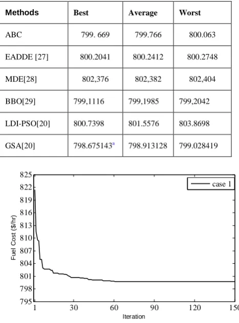
[image:4.595.316.550.358.674.2]The solution details for the minimum cost are provided in Table I, the average cost of solution obtained was 799.766$/hr with the minimum being 799.66 $/hr 8.8097 MW losses and maximum of 800.063$/hr. Fig 2 shows the convergence curve of ABC– OPF for the trial run that produced the minimum cost solution. It is important to note that all control and state variables remained within their permissible limits.
Table 1. Best control variables settings for different test case
Variable Case 1 Case 2 Case 3 Case 4
PG1 (MW) 177.3762 175.6484 199.5897 139.9926
PG2 (MW) 48.5834 48.8422 50.9467 54.9704
PG5 (MW) 21.3299 21.6699 15 23.9236
PG8 (MW) 20.958 22.4669 10 33.2779
PG11 (MW) 11.9622 12.6419 10. 18.4633
PG13 (MW) 12 12.00 12 19.4613
VG1 (pu) 1.1 1.0421 1.0134 1.1
VG2 (pu) 1.0839 1.0276 0.9849 1.0802
VG5 (pu) 1.0548 1.0169 0.9865 1.0531
VG8 (pu) 1.0573 1.0020 0.97 1.0615
VG11 (pu) 1.1 1.0630 1.0254 1.1
VG13 (pu) 1.1 1.0451 1.1 1.1
T6-9 1.04 0.97 1.01 1.02
T6-10 0.90 0.93 1.1 0.90
T4-12 1.04 0.99 0.90 1.03
T27-28 0.97 0.94 0.90 0.97 Fuel Cost
($/h) 799.669 803.9613 930.1114 646.566
Loss
(MW) 8.8097 9.8693 14.1364 6.6891
Σ|Vi-Vref| 1.271 0.0193 0.5815 1.1172
Table 2. Comparison of the simulation results for CASE-1
Methods Best Average Worst
ABC 799. 669 799.766 800.063
EADDE [27] 800.2041 800.2412 800.2748
MDE[28] 802,376 802,382 802,404
BBO[29] 799,1116 799,1985 799,2042
LDI-PSO[20] 800.7398 801.5576 803.8698
[image:4.595.316.547.358.672.2]GSA[20] 798.675143a 798.913128 799.028419
Fig. 2. Convergence curve of the OPF-ABC to Case 1
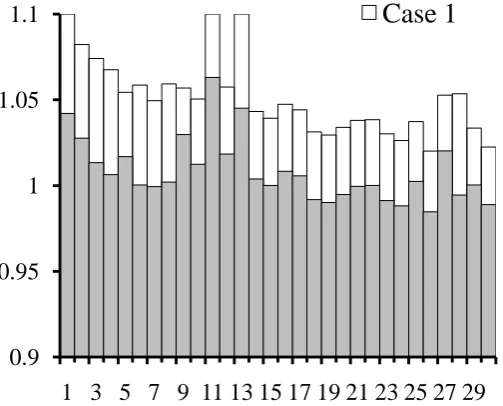
2. Case.2: voltage profile improvement
Bus voltage is one of the most important security and service quality indices. Considering only cost-based objectives in OPF problem may result in a feasible solution that has unattractive voltage profile. So, in this case a two-fold objective function will be considered in order to minimize the fuel cost and improve voltage profile by minimizing the load
1 30 60 90 120 150
795 798 801 804 807 810 813 816 819 822 825
Iteration
F
u
e
l
C
o
st
(
$
/h
r)
[image:4.595.51.286.678.768.2]bus voltage deviations from 1.0 per unit. The objective function can be expressed [19]:
2
1 1
, 1.0
NPQ NG
i Gi i Gi i i
i i
f x u a P b P c V
(18)where
is a suitable weighting factor, to be selected by the user. Value of
in two test systems is chosen as 100. The optimal setting of the control variables are given in Table I. Voltage profile in this case is compared to that of case (1) as shown in Fig 3; It is quite evident that the voltage profile is improved compared to that of Case (1), and if somebody throw a glance at Fig 3 remark clearly that the voltage magnitudes in load buses: 3,4,6,7,12,14, 28 and 29 related at case (1), overtaken the upper limit fixed at 1.05 in pu, with 2.29%, 1.67%, 0.81%, 0.65%, 1.33%, 0.25%, and 0.33%, respectively, this is justified by the strategy of penalty function which presents no problems when enforcing soft limits. However in case (2), all overtaking signaled previously in case (1) are closer at 1 pu. (See Fig 3). [image:5.595.47.299.391.594.2]It is decreased from 1.271 pu in Case (1) to 0.0193 pu in case (2). The result obtained from the proposed algorithm reduces 98.4815% in this case. Table III summarizes the comparison results of the voltage profile improvement. Table IV list lists the statistical results in terms of the best, mean, and worst voltage deviation. From these results, it is clear that ABC obtained a lower value and has a better than those reported in the literature.
Fig. 3. System Voltage Profile
Table 3. Comparison of the simulation results for CASE-2
Variable PSO [27] GSA[20] ABC
PG1 (MW) 173.68 173.32094 175.6484 PG2 (MW) 49.10 49.2639 48.8422 PG5 (MW) 21.81 21.56779 21.6699 PG8 (MW) 23.30 23.2745 22.4669 PG11 (MW) 13.88 13.7745 12.6419 PG13 (MW) 12.00 11.9643 12.00
VG1 (pu) 1.0142 1.0269 1.0421 VG2 (pu) 1.0022 1.00998 1.0276 VG5 (pu) 1.0170 1.0142 1.0169 VG8 (pu) 1.0100 1.00868 1.0020 VG11 (pu) 1.0506 1.05028 1.0630 VG13 (pu) 1.0175 1.01634 1.0451
QG1 (MVA) - - -9.4195
QG2 (MVA) - - 20.0582
QG5 (MVA) - - 48.8269
QG8 (MVA) - - 36.9327
QG11(MVA) - - 17.1459
QG13(MVA) - - 20.0499
T6-9 1.0702 1.07133 0.97
T6-10 0.9000 0.9000 0.93
T4-12 0.9954 0.9965 0.99
T27-28 0.9703 0.9732 0.94
Total Fuel
Cost ($/h) 806.38 804.31484 803.9613 Losses (MW) 10.37 9.76593 9.8693
[image:5.595.51.282.639.761.2]VD 0.0891 0.093269 0.0193
Table 4. Comparison of the simulation results for CASE-2
Methods
Voltage profile improvement
Best Average Worst
ABC 0.0193 0.02777 0.0497
GSA [20] 0.093269 0.093952 0.094171
BBO [29] 0.1020 0.1105 0.1207
PSO [26] 0.0891 NA NA
DE [30] 0.1357 NA NA
3. Case 3: Quadratic cost curve model with sine Component
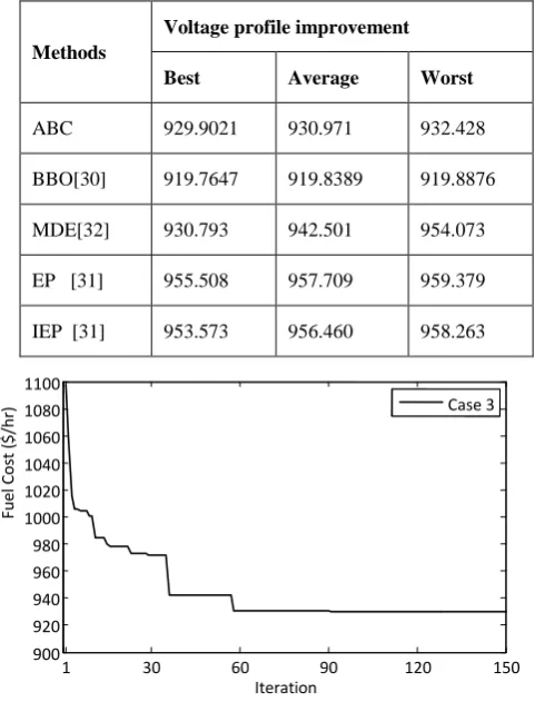
In this case, the generating units of buses 1 and 2 are considered to have the valve-point effects on their characteristics. The cost coefficients for these units are given in Reference [27]. The fuel cost coefficients of the rest generators have the same values as a case (1). The voltage magnitude of generator is set to 0.95Vi 1.1.The maximum and minimum voltages of all load buses are considered to be 1.05 - 0.95 in pu. Limits of transformer tap settings are taken as 0.90Vi 1.1 p.u with an adjustable step size of 0.01p.u. The set of optimal solutions of control variables are presented in Table I. The comparison results are presented in Table V. From simulation results it is very obvious that ABC algorithm has better quality of solutions than EP, IEP, MDE and BBO. It is clear that the minimum fuel cost obtained from the proposed algorithm is 929.902 $/h
0.9
0.95
1
1.05
1.1
1 3 5 7 9 11 13 15 17 19 21 23 25 27 29
with an average cost of 930.971 $/h and a maximum cost of 932.428 $/h, which is less than MDE algorithm and is more than BBO algorithm. But the sum of real power of generating units was given as 294.464MW in BBO approach and real power loss was 12.18MW whereas load was 283.4 MW. So power generation is not matching load plus losses. This approach did not meet the load demand for this case [20]. The convergence curve of ABC algorithm for the OPF problem with minimum fuel cost is shown Fig 4.The results obtained confirm the ability of the proposed ABC algorithm to find accurate OPF solutions in this case study.
Table 5. Comparison of the simulation results for CASE-3
Methods
Voltage profile improvement
Best Average Worst
ABC 929.9021 930.971 932.428
BBO[30] 919.7647 919.8389 919.8876
MDE[32] 930.793 942.501 954.073
EP [31] 955.508 957.709 959.379
IEP [31] 953.573 956.460 958.263
Fig. 4. Convergence curve of the OPF-ABC to Case 3
The cost coefficients for these units are given in Ref [9]. The cost characteristics of the first and second generators are defined in equation (10). The proposed algorithm is applied to this case considering the limit of controls variables has the same limits as a third Case. The results obtained optimal settings of control variables for this case study are listed in Table I, which shows that the ABC has best solution for minimizing of fuel cost in the OPF problem. The best fuel cost result obtained from the ABC approach is compared with other algorithms in Table VI. The average cost of solution obtained was 648.6970$/hr with the minimum being 646.891$/hr and maximum of 650.9820$/hr. According to results of the third and fourth cases, it appear that ABC algorithm has better results compared to other algorithms previously reported in the literature.
Table 6. Comparison of the simulation results for CASE-4
Outputs
CASE-4 Piecewise
DGA[8]
DE[28] IEP [30] MDE
[28]
ABC
PG1 139.95 139.96 139,996 140.00 140.00
PG2 55.00 54.984 54.9849 55.00 55.00
PG5 23.28 23.910 23.2558 24.000 25.9317
PG8 34.36 34.291 34.2794 34.989 34.3422
PG11 19.16 21.161 17.5906 18.044 16.6520
PG13 18.85 16.202 20.7012 18.462 18.1906
Total (MW)
290.60 290.509 290.808 290,495 290.116
Fuel Cost 648.40 648.38 649.312 647.846 646.890
Losses
(MW) 7.204 7.109 7.4081 7.095 7.0527
IEEE 57- bus test System
In order to verify the robustness and efficiency of the proposed algorithm to the larger power system, the algorithm was tested and examined to standard IEEE 57-bus test system. The system has totally 27 variables to be optimized, including 7 generators, 17 transformers (treated as tap changer), and 3 capacitor banks installed at buses 18, 25 and 53 respectively. The total load demand of system is 1250.8 MW and 336.4 Mvar under the base of 100 MVA. The bus 1 is selected as slack bus. The single line diagram of this system and the bus data and line data can be retrieved at MATPOWER [33]. The maximum and minimum voltages of all buses are considered to be 0.95 – 1.1 in p.u. The operating range of all transformers is set between 0.90 -1.1. The minimum and the maximum of shunt capacitor banks are 0.0 and 0.3 in p.u. The control parameter settings of the ABC algorithm related to this case study are provided in Table VII below:
Table 7. Control parameter settings
Parameter IEEE57-Bus
Population size (NP) 40
Max. Cycle number (MCN) 200
Penalty factor of slack bus real power (KP) 1000
Penalty factor of reactive power (KQ) 100
Penalty factor of voltage magnitudes (KV) 100.000
Penalty factor of transmission line loadings (KS) 50
1 30 60 90 120 150
900 920 940 960 980 1000 1020 1040 1060 1080 1100
Iteration
Fue
l Cos
t (
$/hr
[image:6.595.45.286.208.524.2]The set of optimal solutions of control variables from the proposed algorithm are presented in Table VIII. From this Table, it is clear that the best solution of presented result is that of the GSA marked "a", and he is much less than solution obtained by ABC algorithm but is indeed an infeasible solution, since there exist bus voltage magnitude violations at buses 18,19, 20, 26, 27, 28, 29, 30, 31, 32, 33,42,51,56 and 57 and the true value for the total fuel cost corresponding to the set of optimal solutions of control variables reported by GSA is 45621.4035 $/hr.
[image:7.595.322.535.74.218.2]The obtained results are compared with that of the particle swarm optimization (PSO), Cuckoo Optimization Algorithm (COA), LDI-PSO, EADDE, GSA and MATPOWER. This comparison confirms the aptitude of the artificial bee colony algorithm to locate de global solution. Fig 5 shows the convergence curve related to improvement of voltage profile (case 2). Also, it is important to note that all optimization variables remained within their permissible limits without any violations.
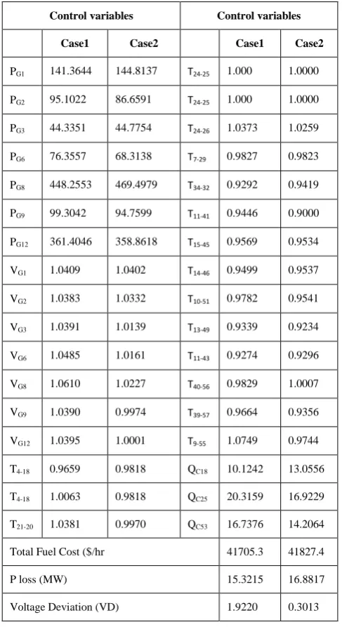
Table 8. The simulation results for CASE 1&2 - IEEE 57
Control variables Control variables
Case1 Case2 Case1 Case2
PG1 141.3644 144.8137 T24-25 1.000 1.0000
PG2 95.1022 86.6591 T24-25 1.000 1.0000
PG3 44.3351 44.7754 T24-26 1.0373 1.0259
PG6 76.3557 68.3138 T7-29 0.9827 0.9823
PG8 448.2553 469.4979 T34-32 0.9292 0.9419
PG9 99.3042 94.7599 T11-41 0.9446 0.9000
PG12 361.4046 358.8618 T15-45 0.9569 0.9534
VG1 1.0409 1.0402 T14-46 0.9499 0.9537
VG2 1.0383 1.0332 T10-51 0.9782 0.9541
VG3 1.0391 1.0139 T13-49 0.9339 0.9234
VG6 1.0485 1.0161 T11-43 0.9274 0.9296
VG8 1.0610 1.0227 T40-56 0.9829 1.0007
VG9 1.0390 0.9974 T39-57 0.9664 0.9356
VG12 1.0395 1.0001 T9-55 1.0749 0.9744
T4-18 0.9659 0.9818 QC18 10.1242 13.0556
T4-18 1.0063 0.9818 QC25 20.3159 16.9229
T21-20 1.0381 0.9970 QC53 16.7376 14.2064
Total Fuel Cost ($/hr 41705.3 41827.4
P loss (MW) 15.3215 16.8817
[image:7.595.314.542.253.462.2]Voltage Deviation (VD) 1.9220 0.3013
[image:7.595.47.291.296.743.2]Fig. 1. Convergence curve of the OPF-ABC to IEEE 57 bus
Table 9. Comparison of the simulation results
Approaches
Fuel cost ($/hr)
Case 1 Case 2
BASE-CASE [32] 51347.86 NA
PSO [31] 42109.7231 NA
COA[32] 41901.9977 NA
LDI-PSO [31] 41815.5035 NA
EADDE [30] 41713.62 42051.44
GSA [20] 41695.8717a NA
ABC 41705.3 41827.4
a
infeasible solution
Table 10. Maximum power flow limit of transmission line of the IEEE 57 bus
Line Smax Line Smax
1 150 7 100
2 85 8 200
3-4 100 9-13 50
5 50 14 100
6 40 15 200
16-80 100
5.
CONCLUSION
A simple Artificial Bee Colony algorithm is proposed to solve the OPF problem under different formulations and considering different objectives function. The performance of the proposed ABC was tested on the IEEE 30-bus test and IEEE 57 test systems. The results obtained using the ABC algorithm were compared to other methods previously reported in the literature.
1 50 100 150 200
1 2 3 4 5 6 7 8 9 10x 10
5
[image:7.595.314.542.493.684.2]The comparison verifies the influentially of the proposed ABC approach over stochastic techniques in terms of solution quality for the OPF problem and confirmed its potential for solving a most nonlinear problems.
6.
ACKNOWLEDGMENTS
The authors like to thank Ministry of Higher Education and Scientific Research (MESRS), ALGERIA that provides an open access to the scientific research resources of the SNDL.
7.
REFERENCES
[1] J. Carpentier, Contribution `a l'etude du dispatching ´economique. Bulletin de la Soci´et´e Fran¸caise des ´ Electriciens, Vol.3, pp:431–447, August 1962.
[2] T. Niknam, M. Narimani. R, A-Abarghooee. A new hybrid algorithm for optimal power flow considering prohibited zones and valve point effect,” Elsevier-Energy Conversion and Management, Vol. 58, pp, 197-206. (Feb, 2012).
[3] G. B. S. David C, Walters, “Genetic algorithm solution of economic dispatch with valve point loading,”. IEEE Transactions on Power Systems. Vol, 8, No, 3, August, pp, 1325-1332, Aug, 1993.
[4] Wen-Hsiung E. Liu, Alex D. Papalexopoulos, William F. T h e y, “ Discrete shunt controls m a newton optimal power flow,” Transactions on Power Systems. Vol. 7, No. 4. PP 1509 – 1518, November 1992.
[5] Alex d. papalexopoulos carl f, imparato felix f. wu, “large-scale optimal power flow: effects of initialization, decoupling & discretization,” IEEE transactions on Power Systems. Vol. 4, No. 2, PP. 748- 759, May 1989. [6] J. A. Momoh, M. E. Elhawary, and R. Adapa. “A
review of selected optimal power flow literature to 1993 part1: nonlinear and quadratic programming approaches,”IEEE Trans Power System. vol4, N 1, pp, 96- 104, 1999.
[7] B.Mahdad, T. Bouktir, K. Srairi, and M. EL. Benbouzid, “Dynamic strategy based fast decomposed GA coordinated with FACTS devices to enhance the optimal power flow,”. Energy Conversion and Management,
Vol.51, pp,1370–1380.
doi:10.1016/j.enconman.2009.12.018. (2010).
[8] B.Mahdad, K. Srairi, T. Bouktir and M. EL. Benbouzid, “ Optimal Power Flow with discontinous Fuel Cost Functions Using Decomposed GA Coordinated with Shunt FACTS,”, Journal of Electrical Engineering & Technology. Vol 4, pp.457-466.
[9] Abido M.A, “Optimal power flow using particle swarm optimization,” Electric Power Energy System 2002, Vol. 24:563-71.
[10]Leandro. dos Santos. Coelho, Viviana. Cocco. Mariani, “Combining of Chaotic Differential Evolution and Quadratic Programming for Economic Dispatch Optimization With Valve-Point Effect,” IEEE Transactions on power systems, vol, 21, No, 2, May 2006.
[11] Jason .Yuryevich, Kit. Po. Wong, “Evolutionary Programming Based Optimal Power Flow Algorithm,” IEEE Transactions on Power Systems, vol, 14, No, 4, pp, 1245-1250, Nov, 1999.
[12]P.K. Roy , S.P.Ghoshal, S.S. Thakur, “Biogeography based optimization for multi-constraint optimal power flow with emission and non-smooth cost function,” Elsevier-Expert Systems with Applications, No, 37, p, 8221–8228, 2010.
[13]D. Karaboga, B. Basturk, “A powerful and Efficient Algorithm for Numerical Function Optimization": Artificial Bee Colony (ABC) Algorithm,” Journal of Global Optimization, Vol.39, No 3, pp. 459-171, November 2007.
[14]D. Karaboga, B. Basturk, “On The Performance Of Artificial Bee Colony (ABC) Algorithm,” Applied Soft Computing,Vol 8, No 1, pp. 687-697, January 2008. [15]Mohd. Afizi, Mohd. Shukran, Yuk. Ying. Chung,
Wei-Chang. Yeh, Noorhaniza Wahidand and Ahmad Mujahid. Ahmad. Zaidi “Artificial Bee Colony based Data Mining Algorithms for Classification Tasks,” Modern Applied Science. Canadian Center of Science and Education 5, 217–231, (2011).
[16]D. Karaboga, B. Akay, “A modified artificial bee colony (ABC) algorithm for constrained optimization problems,” Applied Soft Computing, Vol 11, Issue 3 , pp. 3021–3031, April 2011.
[17]A.Singh, “An artificial bee colony algorithm for the leaf-constrained minimum spanning tree problem,”" Applied Soft Computing, Vol 9, Issue 2, pp. 625-631, 2009. [18] N. Karaboga, “A new design method based on artificial
bee colony algorithm for digital IIR filters,” Journal of the Franklin Institute, vol. 4, pp. 328-348, 2009.
[19]C. Xu, and H. Duan, “Artificial bee colony (ABC) optimized edge potential function (EPF) approach to target recognition for low-altitude aircraft,” Pattern Recognition Letters, pp. 1759-1772, 2010.
[20]Serhat. Duman, Ugur. Güvenç, Yusuf. Sönmez, Nuran Yörükeren, “Optimal power flow using gravitational search algorithm,” Elsevier - Energy Conversion and Management, No, 59, pp, 86–95, Feb, 2012.
[21]Nima. Amjady , Hossein Sharifzadeh, “Solution of non-convex economic dispatch problem considering valve loading effect by a new Modified Differential Evolution algorithm,” Electrical Power and Energy Systems, No, 32, p, 893–903, Jan, 2010.
[22]P. Saravuth, N. Issarachai, K. Waree, “Application of multiple tabu search algorithm to solve dynamic economic dispatch considering generator constraints,” Elsevier- Energy Conversion and Management, No, 49, pp, 506–516, Aug, 2008.
[23]D. Karaboga, “An idea based on honey bee swarm for numerical optimization”, Technical Report Tr06, Erciyes University, Engineering Faculty, Computer Engineering Department 2005.
[24]D. Karaboga and B. Basturk, “Artificial Bee Colony (ABC) Optimization Algorithm for Solving Constrained Optimization,” Springer (Verlag Berlin Heidelberg), pp, 789–798, 2007.
[26]K. Vaisakh. LR. Srinivas, “Evolving ant direction differential evolution for OPF with non-smooth cost functions,” Engineering. Applications of Artificial Intelligence Vol. 24, pp.426–36. 2011
[27]S. Sayah, K. Zehar, “Modified differential evolution algorithm for optimal power flow with non-smooth cost functions,” Elsevier- Energy Conversion and Management. Vol 49, pp.3036–3042. 2008
[28]A. Bhattacharya, PK. Chattopadhyay, “Application of biogeography-based optimization to solve different optimal power flow problems,” IET Generation, Transmission & Distribution. Vol. 5, pp.70–80. 2011, doi: 10.1049/iet-gtd.2010.0237.
[29]W. Ongsakul, T. Tantimaporn. “Optimal power flow by improved evolutionary programming,” Electr Power Components Syst. Vol. pp.34, 79–95. 2006. M. Pandian. Vasant. “Meta-Heuristics Optimization Algorithms in Engineering, Business, Economics, and Finance,” Petronas University of Technology, Malaysia. Chapter 1 by (Dieu Ngoc Vo, Peter Schegner) Book. pp 1-40. 2013. [30]K. Vaisakh, L.R. Srinivas. “Evolving ant direction differential evolution for OPF with non-smooth cost functions,” Engineering Applications of Artificial Intelligence. Vol.24 pp.426–436. 2011.
[31]M. Rezaei Adaryani, A. Karami, “Artificial bee colony algorithm for solving multi-objective optimal power flow problem,” Electrical Power and Energy Systems Vol.53, pp. 219–230. 2013.
[32]Hisashi. Handa, Hisao Ishibuchi, Yew-Soon Ong, Kay Chen Tan. “Proceedings of the 18th Asia Pacific Symposium on Intelligent and Evolutionary Systems,” – Vol 1. Springer International Publishing Switzerland. pp 479-493. 2015.
[33]MATPOWERhttp://www.ee.washington.edu/research/pst ca/
[34]Avadhanam Kartikeya Sarma, Kakarla Mahammad Rafi. “Optimal Capacitor Placement in Radial Distribution Systems using Artificial Bee Colony (ABC) Algorithm” Innovative Systems Design and Engineering, Vol 2, No 4, 2011.