Vol. 04, Issue 02 (February. 2014), ||V6|| PP 35-42
Fast Detection of Connected Components in Large Scale Graphs
Using MapReduce
Ali Varamesh
1, Mohammad Kazem Akbari
11Computer Engineering and Information Technology Department
Amirkabir University of Technology, Tehran, Iran
Abstract: - Finding connected components of a graph is a fundamental problem in graph theory which arises in many different applications including data mining and network analysis. By increasing popularity of social networks and information systems, scale of real world graphs have increased to billions of nodes and edges. Thus, finding connected components of large scale graphs turned to be a computationally challenging task. Because of this, in recent years, there has been some works addressing this problem using the well-known MapReduce distributed large scale data processing framework. However, they do not have acceptable performance and sstill tere is great potential for imporvments. In this paper, we introduce a new approach for finding connected components of large scale graphs using MapReduce framework. Based on the results of the experiments on real-world datasets, we show that, by using the new algorithm, significant performance improvements have been gained. We also explain that the main idea of our algorithm is based on a general theory for effective utilization of computational resources provided by nodes in a MapReduce cluster to reduce communication and IO load.
Keywords: -Complex Networks, Connected Components, Large Scale Graph Processing, MapReduce
I.
INTRODUCTION
Large scale graphs are popular in modern information systems such as social networks, scientific networks, e-commerce systems, web graphs, and etc which contain graphs of billion scales. Such graphs should be analyzed using graph procesing data mining methods in order to extract valuable information such as community structure of a social network, trend prediction in an academic research field, and ranking web pages to name a few. One of the basic algorithms used in graph mining is finding connected components of a graph which also has some other forms such as S-T Connectivity. There have been many sequential algorithms to find connected components of graphs, but finding connected components of real world graphs has became a challenging task in recent years due to their very large scale size. One approach to tackle this challenge is to use parallel and distributed computing.
Many parallel and distributed approaches have been proposed to solve this problem [1], [4], [6], [7] and [8]. Especially, some algorithms are designed using MapReduce distributed computing framework, which in recent years has been extensively used in large scale data processing. However, these MapReduce based algorithms still has potential to significant optimizations. In this paper we introduce a new algorithm which is essentially an improvement over PEGASUS, a popular MapReduce algorithm for finding connected components of large scale graphs. The new algorithm reduces amount of intermediate MapReduce data and the number of iterations that PEGASUS takes to complete. According to experiments, the new algorithm significantly outperforms the state-of-the-art algorithms.
In the rest of this paper, section 2 introduces MapReduce framework. Then, section 3 analyses the related works and presents motivations for the new algorithm. Section 4 introduces the new MapReduce algorithm for finding connected components, followed by the experimental results and discussion on them in section 5. We conclude the paper and give some directions for future work in section 6.
II.
THE
MAPREDUCE
COMPUTATIONAL
MODEL
MapReduce has emerged as a new paradigm in distributed large scale data processing in recent years [2]. Scalability, load balancing, and fault tolerance are its most important characteristics. It has been used to solve computationally challenging problems in many fields, for example, large scale graph processing problems such as PageRank and maximum clique enumeration problem [4], [9]. MapReduce framework increases scale by leveraging large number of loosely synchronized machines each processing a fraction of data in parallel.
the shuffle phase sends all values associated with a key to a same reducer. The shuffle phase is the only synchronization required between Map and Reduce phases and all tasks during each phase work independently.
The MapReduce framework assumes that input data is split over a distributed cluster file system and then executes the Map function on each split. Amount of intermediate data generated between map and reduce phases is a bottleneck for performance and scalability. Simply, because it should be sorted using an external sorting algorithm and then sent to the right reducer through the network. As the amount of intermediate data increases, I/O and communication load also increase. Therefore, reducing amount of intermediate data would result in significant performance improvements. In addition, finding connected components using MapReduce is an iterative task and reducing number of iterations also would result in performance improvement. In the next section we present our approach which decreases amount of intermediate data and number of iterations.
III.
RELATED
WORKS
AND
MOTIVATIONS
There have been some works which developed MapReduce algorithms to find connected components of large scale graphs [1], [3], [6], [7]. Among them, two algorithms are most successful and popular and we will describe them in detail. These algorithms are based on some kind of label propagation. They assign a numerical component ID to each node and neighbor nodes of the graph exchange their component IDs until each node gets its right component ID. Our new algorithm also is based on this label propagation approach and actually our work will be an improvement on computational aspects of this approach. Before describing our algorithm, first we introduce two mentioned algorithms.
3.1. Related Works
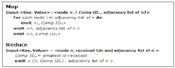
The most popular work in this area is done by Kang et al [3]. Their MapReduce algorithm, PEGASUS, is showed in the code below. They have introduced a MapReduce model of matrix-vector multiplication to implement their algorithm, but their implementation method is not our concern at this work. PEGASUS initially sets component ID of each node to be the node’s ID. Then in map phase of the following iterations, each node sends its component ID to its neighbors. In the reduce phase each node sets its component ID to smallest component ID among those IDs it received and its ID set in the previous iteration. The algorithm iterates until component ID of none of the nodes changes.
In [6] two new algorithms are introduced which aim at reducing the number of rounds in finding connected components using MapReduce. Based on the experiments presented in their paper, one of their algorithms, named as Hash-to-Min, has the best performance regarding run time. In the initialization step, the algorithm assumes that each node and its neighbors constitute a connected component. In map phase of the following iterations, each node sends IDs of all members of the component associated with it to the member with smallest ID and sends the smallest node ID to other nodes. Then in the reduce phase, each node receives the members associated with it and stores it. The algorithm terminates when all nodes are associated with the node with smallest ID in the component which they belong to. Therefore, at each iteration, all nodes of a component should be sent to the reducer which processes the member of the component with smallest ID. This would cause unbalanced computational and communication load to be directed to some reducers. In the case of existence of huge components, which is popular in real world graphs [6], there would be significant lack of performance and scalability. However, they also have devised some solutions to smooth this problem.
Seidl et al [7] also have introduced an algorithm called CC-MR which is essentially based on the same approach as of Hash-to-Min. They have also devised an elegant solution to counter the intrinsic unbalanced load distribution associated with the approach. Moreover, they have released an open-source version of their implementation. However, this approach still does not have satisfying performance in case of large scale graphs.
3.2 Motivations
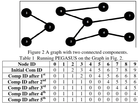
As mentioned, reducing amount of intermediate data and number of iterations will cause significant performance achievements. Thus we concentrate on reducing I/O and network communication load of PEGAUS. In the mean while our approach would decrease the number of iterations it take to find connected components of a graph. As the experiments shows, the new algorithm generates less intermediate data and terminates in less number of iterations than PEGASUS. Further the new algorithm shows much better performance than CC-MR and Hash-to-Min. First we show how PEGASUS operates on a graph. As an example of the algorithm’s procedure, we describe its operation over the graph presented in
Table 1 Running PEGASUS on the Graph in Fig. 2.
Node ID 0 1 2 3 4 5 6 7 8 9
Initial Com ID 0 1 2 3 4 5 6 7 8 9
Comp ID after 1st 0 1 1 2 0 4 5 6 6 8
Comp ID after 2nd 0 1 1 1 0 0 4 5 5 6
Comp ID after 3rd 0 1 1 1 0 0 0 4 4 5
Comp ID after 4th 0 1 1 1 0 0 0 0 0 4
Comp ID after 5th 0 1 1 1 0 0 0 0 0 0
Fig. 1. Suppose that at each iteration there are two mapers and one reducer and nodes 0 to 4 will be processed by first maper and the other nodes by the second maper. As presented in Table 1, PEGASUS initially sets the component ID of each node to be same as its node ID. Then in map phase of the first iteration node 6, for example, sends its component ID to all its neighbor nodes, which is 3, 5, and 8. In the reduce phase, node 6 also receives component ID of its neighbors and sets its component ID to be 5 which is the smallest ID among those it received and its current component ID. Component IDs of other nodes after the first iteration are presented in Table 1.
IV.
MEMORYCC:
THE
NEW
FAST
ALGORITHM
In MapReduce each map and reduce task processes its input records one by one. Each record has two parts, key and value. In the Fig. 1 it has shown that a node’s ID is constitutes the key part of a record and component ID plus adjacency list of the node constitutes the value part. As an illustration of how map function operates on an input record, when in the second iteration the second maper receives the record <5, (0,{4,6})> it produces the four new records as intermediate data: <4, 0>, <5, 0>, <6, 0>, <5, {4, 6}>. By the first and third record it sends current component ID of node 5 that is 0, to the 4 and 6. By the second record it preserves the current component ID of node 5 because in reduce phase it may not receive any smaller ID from its neighbors. And by the last record the algorithm maintains the graph structure to be used in the following iterations. In reduce phase of the second iteration node 6 will set its component ID to 0 because it is the smallest ID it receives. Then in the map phase of the third iteration the node 6 will tell to is neighbors that its component ID is 0 which causes them to set their component Id to 0 in the reduce phase of the third iteration. The algorithm will continue in the same way until it terminates.
As you can see, in map phase of each iteration each record is processed by a map task and the task does not have any assumption about the other records which it processes at the same iteration. But, in MapReduce each map task could firt load all of its input records to a hash map and then access to the data structure during its lifetime [5]. We use this feature to improve PEGASUS algorithm. Now we describe our method step by step. In the remainder of this paper we refer to our method as MemoryCC.
The initialization step of MemoryCC is same as that of PEGASUS. At each iteration of MemoryCC, first each maper loads all of its input records into a hash map data structure called SubGraph. In addition, it separates adjacency list of each into two parts. Part one contains those adjacent nodes which are processed by the
and one reducer we run MemoryCC over the graph in Fig. 1. At each iteration, the first maper processes nodes with IDs 0 to 4 and the second maper processes nodes with IDs 5 to 9. After loading input records to SubGraph, each mapers starts the main part of its procedure. In contrast to PEGASUS, each maper has simultaneous access to all of its input records. For example, when the first maper processes node 0, it has access to node 4 and thus, does not emit the record <4, 0> to tell its component ID to node 4. Instead, it tell directly to node 4 that its neighbor’s component ID is 0. This means that neighbor nodes which are processed by the same maper do not need to send their component ID to each other through the reduce phase. Therefore, because 0 is smaller than previous component ID of node 4, that is 4, the maper will update component ID of node 4 to 0. Each maper applies this procedure on all its internal nodes and if a node has an internal neighbor with a smaller component ID, the maper replaces the node’s component ID with its neighbor’s component ID. This procedure will repeat until component ID of none of the internal nodes updates.
In contrast to PEGASUS, when generating intermediate records in MemoryCC, current component ID of each internal node is updated during the map phase. In addition, the maper sends to each external node the smallest component ID among the component IDs of the node’s neighbors among internal nodes. Outputs of the first and second mapers are shown in Table 2. The reduce function of MemoryCC will be same as the reduce function of the PEGASUS. Table 3 presents the final output of MemoryCC after each iteration. As you can see, MemoryCC finds connected components of the graph in Fig. 1 in two rounds while PEGASUS takes five iterations to complete.
Table 2 Output of Mappers in the First Iteration of Execution of MemoryCC on the Graph of Fig. 2.
Output records of the first maper Output records of the second maper
<0, 0 >, <0, {4}>, <1, 1>, <1, {2}>, <2, 1 >, <2, {1, 3}>, <3, 1 >, <3, {2}>, <4, 0 >, <5, 0 >, <4,
{0, 5}>
<5, 5 >, <4, 5 >, <5, {4, 6}>, <6, 5 >, <6, {5, 7, 8}>, <7, 5 >, <7, {6}>, <8, 5>, <8, {6, 9}>, <9,
5>, <9, {8}>
Table 3 Output of each iteration when running MemoryCC on the graph of Fig. 2.
As a general description of MemoryCC, it partitions the input graph to sub graphs and each maper loads the sub graph associated with it into a hash map data structure called SubGraph. Thanks to this, at each iteration of MemoryCC, every maper finds connected component of nodes in the sub graph associated with it. As an illustration, in the example of the graph of Fig. 1, at the first iteration, the first maper finds two connected components in the first sub graph. One consisted of nodes 0 and 4 and the other consists of nodes 1, 2, and 3 with 0 as and 1 set as component IDs respectively and the second maper detects that the whole sub graph associated with it, is a connected component with 5 as component ID. Then each connected component sends it’s ID to external nodes which is neighbor with. This makes it possible to connected components found on different mapers to merge in reduce phase if they are connected through some edge. This idea is essentiall same as the idea introduced in [10]. The next section presents the experimental results and discussion about them.
V.
EXPERIMENTS AND DISCUSSION
This section presents experiments and discussion about benchmarking MemoryCC and other algorithms against real world data sets. All of the experiments are done on a Hadoop cluster consisting of 8 nodes connected to each other through a one gigabit Ethernet LAN, each with 8 processing cores and 16 gigabytes of memory. Statistics of the data sets we have used are presented in Table 4. All datasets are available through the web page of Stanford Network Analysis Project (SNAP). We have implemented our algorithm on Apache Hadoop which is an source implementation of MapReduce framework. For PEGASU and CC-MR we have used their open-source and free implementations respectively.
Node ID 0 1 2 3 4 5 6 7 8 9
Initial Com ID 0 1 2 3 4 5 6 7 8 9
Comp ID after 1st 0 1 1 1 0 0 5 5 5 5
VI.
Table 4 Statistic of data sets used in experiments.
Dataset Nodes Edges Diameter Size in MB
com-amazon 334863 925872 44 14.2
com-DBLP 317080 1049866 22 15.3
com-YouTube 1134890 2987624 21 44.5
as-Skitter 1696415 11095298 25 154.1
com-LiveJournal 3997962 34681189 18 507.8
com-Orkut 3072441 117185083 8 1740.8
5.1 Memory Usage
As we described, each maper of MemoryCC loads the sub graph associated with it into memory. At first this may be seemed problematic due to its high memory usage, but even in clusters made up of commodity hardware, each node usually has up to many gigabytes of memory per processing core. In addition, real world data sets usually are of gigabytes in size and whole of them could be loaded even into memory associated with one maper. For example, the largest data set we have used is com-Orkut which is 1.7 gigabytes. Considering that two gigabytes of memory is available for each maper in our cluster, even whole of com-Orkut data set could be load into memory of one maper. In addition, since we would divide data sets into sub graphs, it is clear that size of sub graphs would be much less than size of the data set itself. For example, in our cluster, we are able to divide each data set among 52 mapers each with to up to two gigabytes of memory which means we are able to process data sets as large as 100 gigabytes. Furthermore, as size of real world data sets grows, memory technology is also advances to support larger amounts of memory per processing core. So it seems neither today nor would in the future available memory be a problematic issue for performance of MemoryCC.
5.2 Performance
Our main approach in developing a new MapReduce algorithm was reducing amount of intermediate data and number of iterations. For example, in case of the graph shown in Fig. 1, MemoryCC completed in half the iterations PEGASUS took to terminate. In addition by loading the sub graphs into memory of mapers the nodes inside mapers do no need to communicate through the reduce phase and they directly share their component ID with each other at the map phase.
Moreover, in case of external nodes, in contrast to PEGASUS, in MemoryCC a maper just sends one message to each of its external nodes. Consequently these result in reduction in amount of intermediate data. Fig. 4 presents amount of intermediate data generated by MemoryCC, PEGASUS, and CC-MR when executed over data sets of
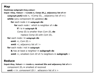
Map
Hashmap subgraph<key,value>
Input <Key, Value> : <(node n, Comp IDn), adjacency list of n>
subgraph.put(node n, <Comp IDn , adjacency list of n>)
while (any component ID updates) do
for each node n in subgraph do
for each node i which is neighbor of ndo if i is in subgraph &
Comp IDi is smaller than Com IDn do
replace Comp IDiwith Com IDn for each node i in subgraph do
emit <i, Com IDi >
emit <i, adjacency list of i >
for each node i not in subgraph
& has at least a neighbor in subgraph do
emit <i, smallest Com ID of i’s neighbors in subgraph >
Reduce
Input<Key, Value> = <node n, received IDs and adjacency list of n >
component IDn = smallest id received
emit < (n, component IDn) , adjacency list of n >
showed in Fig. 4a, the intermediate data generated by MemoryCC is four to twenty times less than PEGASUS and three to ten times less than CC-MR. So MemoryCC significantly reduces amount of intermediate data.
Figure 4 Amount of intermediate data produced by different algorithms.
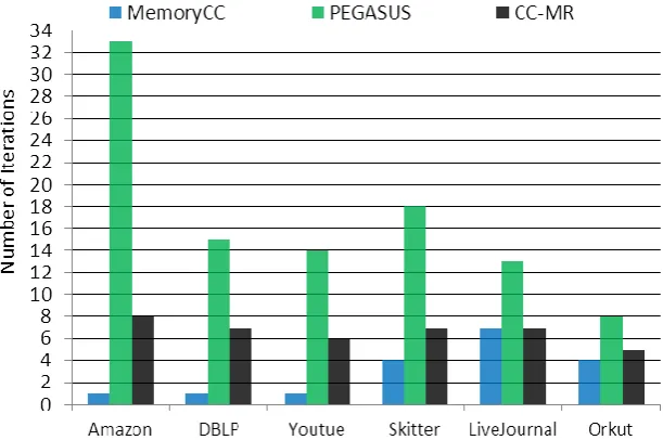
In Fig. 5 number of iterations that different algorithms take to complete when applied over datasets of Table 4 is presented. As you can see, in three of the data sets, that is Amazon, DBLP, and YouTube, MemoryCC just takes one iteration to complete. Not surprisingly, this is because of the fact that these data sets have very small size and MemoryCC partitions them to no more than one sub graph. This means that each of these data sets is processed just by one mapper and this mapper loads whole of the data sets into its memory and then founds connected components of them at the first iteration. On other data sets MemoryCC approximately completes in half the number of iterations that PEGASUS takes to complete. In comparison to CC-MR, also MemoryCC takes smaller number of iterations except the case of LiveJournal data set, on which both algorithms finish in same number of iterations.
Figure 5 Number of iterations that different algorithms take to terminate.
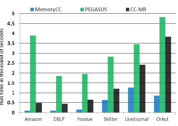
Figure 6 Runtime of different algorithms.
Results show that MemoryCC is up to ten times faster than PEGASUS and CC-MR .It could be proved that the communication complexity of the MemoryCC is O(V), where V is the number of vertices. Since the communication and intermediate data are the most time consuming part of MapReduce algrithms, it is predictable that the runtume of the MemoryCC shoud be in direct relation with the number of nodes. This is shown in Fig. 7 Because the quantity of runtime is very small in comarison to the number of nodes, in this diagram the run time is multiplied by 10000 to scale and shift the runtime curve.
Figure 7 The relationship between runtime and number of nodes.
VII.
CONCLUSION
Although we have shown that MemoryCC has much better performance than the available algorithms, there are some issues which could be worked on in the future. Especially, time and space complexity of MemoryCC could be carefully analyzed and compared with that of other algorithms. In addition MemoryCC seems much more scalable than other algorithms but it is necessary to prove this fact based on theory and more experiment. Furthermore, it seems that partitioning input graphs among mapers may be beneficial if applied to many other graph processing algorithms. Thus, as the future work we concentrate on possibility of improving other MapReduce based graph processing algorithms using the approach used here in designing MemoryCC.
VIII.
ACKNOWLEDGEMENTS
This research has been supported by the Iran Telecommunication Research Center.
REFERENCES
[1] J. Cohen, Graph twiddling in a MapReduce world, Computing in Science & Engineering, 11, 2009, 29-41. [2] J. Dean and S. Ghemawat, MapReduce: simplified data processing on large clusters, Communications of
the ACM, 51, 2008, 107-113.
[3] U. Kang, C. E. Tsourakakis, C. Faloutsos, Pegasus: A peta-scale graph mining system implementation and observations, Proc. 9th IEEE Interntional Conf. on Data Mining, Miami, FL, 2009, 229-238.
[4] U. Kang, C. E. Tsourakakis, C. Faloutsos, Pegasus: mining peta-scale graphs, Knowledge and Information Systems, 27, 2011, 303-325.
[5] J. Lin and M. Schatz, Design patterns for efficient graph algorithms in MapReduce, Proc. 8th ACM Conf. on Workshop on Mining and Learning with Graphs, 2010, 78-85.
[6] V. Rastogi, et al., Finding connected components on map-reduce in logarithmic rounds," arXiv preprint,
2012, arXiv:1203.5387.
[7] T. Seidl, B. Boden, S. Fries, CC-MR–Finding Connected Components in Huge Graphs with MapReduce,
in Springer (Ed), Machine Learning and Knowledge Discovery in Databases, (2012), 458-473.
[8] B. Wu and Y. Du, Cloud-based connected component algorithm, Proc. IEEE Interntional Conf. on Artificial Intelligence and Computational Intelligence, 2010, 122-126.
[9] B. Wu, S. Yang, H. Zhao, B. Wang., A distributed algorithm to enumerate all maximal cliques in mapreduce, Proc. 4th IEEE Interntional Conf on In Frontier of Computer Science and Technology, 2009, 45-51.