A generic capacitated multi-period, multi-product, integrated forward-reverse logistics network design optimization model

(1)

ISSN (e): 2250-3021, ISSN (p): 2278-8719

Vol. 06, Issue 05 (May. 2016), ||V2|| PP 40-56

A generic capacitated multi-period, multi-product, integrated

forward-reverse logistics network design optimization model

M. S. Al-Ashhab

Design & Production Engineering Dept. Faculty of Engineering, Ain-Shams University– Egypt Dept. of Mechanical Engineering, Collage of Engineering and Islamic architecture, UQU, KSA

ABSTRACT: In This Paper, A Generic Capacitated Multi-Product, Multi-Period, Multi-Echelon Integrated

Forward-Reverse Logistics Network Design Is Developed. The Proposed Network Structure Consists Of Three Echelons In The Forward Direction, (Suppliers, Factories, And Distributors) And Two Echelons In The Reverse Direction (Disassembly And Redistribution Centers) To Provide The First Customer Zones With Virgin Products And The Second Customer Zones With Refurbished Ones. The Problem Is Formulated In A Mixed Integer Linear Programming (MILP) Decision-Making Form. The Objective Is To Maximize The Total Profit. The Performance Of The Developed Model Has Been Verified Through Two Examples.

KEYWORDS: Supply Chain; Location Allocation; Reverse Logistics; Forward-Reverse Logistics; MILP; Mixed Integer Linear Programming; Closed Loop.

I. INTRODUCTION

Closed loop or integrated forward reverse network establishes a relationship between the market that releases used or refurbished products and the market for new or virgin products.

Salema, M. I. G. et al. (2007) developed a mixed integer formulation for reverse distribution allows for any number of products, But the inventory was not taken into consideration.

Pishvaee, M. S. et al. (2009) developed a single period single product stochastic programming model for an integrated forward/reverse logistics network design under uncertainty.

El-Sayed, M. et al. (2010) developed a single product stochastic mixed integer linear programming for designing a forward–reverse logistics under demand risk.

Ramezani, M. et al. (2013) presented a single period stochastic multi-objective model for forward/reverse logistic network design under an uncertain environment.

Mutha, A., & Pokharel, S. (2013) proposed a mathematical RLN design model considering a third party collectors.

Hatefi, S. M., & Jolai, F. (2014) formulated a single period, single product robust and reliable model for an integrated forward–reverse logistics network design based on a recent robust optimization approach protecting the network against uncertainty.

Serdar E. T. & Al-Ashhab M. S. (2016) modeled a multi-product, multi-period supply chain network mathematically in a mixed integer linear programming (MILP) form deciding both location and allocation decisions which maximize the total profit.

In this work, a generic multi-product, multi-period multi-echelon integrated forward-reverse logistics network design model is developed. The model is formulated in a mixed integer linear programming (MILP) decision-making form. The objective of the model is to maximize the total profit. Decisions are taken to determine the following:

i. Suppliers, factories, distribution centers, disassembly, and redistribution centers locations, ii. Production volume at each period in each location (what and how much to produce), iii. Transported quantity of goods between locations, and

iv. The quantity of goods to hold as inventory at each period in both the facility and distributor stores.

II. MODEL DESCRIPTION

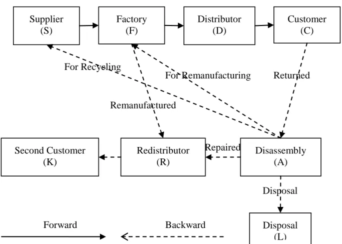
The model is a formulation for the integrated forward-reverse logistics network design problem. The network is a multi-product, multi-period, multi-echelon, where it consists of three suppliers, three factories, three distributors, and four first customers in the forward direction and it consists of three disassembles, three disposal centers, three redistribution locations and second customers in the reverse direction, as shown in Figure 1.

(2)

In the forward direction, the suppliers supply the raw material to the factories which manufacture them and send them to the distributors to send them to the first customer considering their demand. In the reverse direction, the first customers return the used products to the disassembly locations for disassembling, and sorting for supplying the recyclable to the suppliers, the remanufacturable to the factories, the disposable to the disposal locations, and to repair the repairable products and supplying them directly to the redistribution locations. The recycled material is supplied to factories. The remanufactured and repaired products are supplied to the second customers through redistribution locations.

Costs incurred at different locations are as follows are shown in Table 1.

Table 1: Costs incurred at different locations of the network.

Forward Logistics Echelons Cost Elements

Location Suppliers Factories Distributors

Costs

1. Fixed 1. Fixed 1. Fixed

2. Materials 2. Manufacturing 2. Shortage 3. Recycling 3. Remanufacturing 3. Storage 4. Transportation 4. Non-utilized manufacturing capacity 4. Transportation 5. Non-utilized remanufacturing capacity

6. Storage

7. Transportation

Reverse Logistics Echelons Cost Elements

Location Disassembly Redistribution Disposal

Costs

1. Fixed 1. Fixed 1. Fixed

2. Returned price 2. Transportation 2. Disposing

3. Disassembly

4. Inspection

5. Sorting

6. Repairing

7. Transportation

III. MODEL FORMULATION

The model involves the following sets, parameters, and decision variables:

Sets:

Backward Forward

Repaired Supplier

(S)

Factory (F)

Distributor (D)

Customer (C)

Second Customer (K)

Redistributor (R)

Disassembly (A) For Remanufacturing

For Recycling

Disposal Remanufactured

(3)

S, F, D, and C: potential number of suppliers, factories, distributors, and first customers,

A, R, L, and K: potential number of disassembly, redistributors, locations, disposal, and second customers. P: number of products,

T: number of periods.

Parameters:

Dcpt: demand of first customer c from product p in period t, Dkpt: demand of the second customer k from product p in period t, Ppct: unit price of product p at customer c in period t,

Ppkt: unit price of product p at second customer k in period t, Fi: fixed cost of opening location i,

DSij: distance between any two locations i and j, CAPSst: capacity of supplier s in period t (kg),

CAPMft: capacity of raw material store of facility f in period t (kg), CAPHft: capacity in manufacturing hours of facility f in period t, CAPFSft: capacity of final product store of facility f in period t (kg), CAPDdt: capacity of distributor d in period t (kg),

CAPAat: capacity of disassembly a in period t,

CAPRCst: recycling capacity of supplier s in period t (kg),

CAPRMft: remanufacturing capacity in hours of factory f in period t, CAPRrt: capacity of redistributor r in period t,

CAPLlt: capacity of disposal p in period t,

MatCst: material cost per unit supplied by supplier s in period t, RECst: recycling cost per unit recycled by supplier s in period t, MCft: manufacturing cost per hour for factory f in period t, RMCft: remanufacturing cost per hour for factory f in period t,

DACat: disassembly cost per unit weight disassembled by disassembly location a in period t, REPCat: repairing cost per unit repaired by disassembly location a in period t,

DISPClt: disposal cost per unit disposed of by disposal location l in period t, NUCCf: non-utilized manufacturing capacity cost per hour of facility f, NURCCf: non-utilized remanufacturing capacity cost per hour of factory f,

SCPUp: shortage cost per unit per period for product p, MHp: manufacturing hours for product p,

RMHp: remanufacturing hours for product p,

FHf: holding cost per unit weight per period at the store of factory f, DHd: holding cost per unit weight per period at distributor store d,

Bs, Bf, Bd, Ba & Br: batch size from supplier s, factory f, distributor d, disassembly a, and, redistributor r

respectively,

Tc: transportation cost per unit per kilometer, RR: return ratio at the first customers, RC: recycling ratio,

RM: remanufacturing ratio, RP: repairing ratio, RD: disposal ratio,

Decision variables:

Li: binary variable equals 1 if location i is open and 0 otherwise,

Qijpt: flow of batches from location i to location j of product p in period t, Ifpt: flow of batches from factory f to its store of product p in period t,

Ifdpt: flow of batches from store of factory f to distributor d of product p in period t, Rfpt: the residual inventory of product p in the period t at store of factory f, Rdpt: the residual inventory of product p in the period t at distributor d.

3.1. Objective Function

The objective of the model is to maximize the total profit of the forward-reverse network. Total Profit = Total Revenue – Total Cost.

3.1.1. Total Revenue

(4)

   

   



D d c C p P

pct dp dcpt B P

Q Sales First T t

(1)

   

     R r k Cp P

pkt rp rkpt B P

Q Sales Second T t

(2)

   

     A

a s Sp Pt T

st st

p a

ast B W (MatC -REC ) Q

saving cost

Recycling

(3)

3.1.2. Total Cost

Total cost = fixed costs + material costs + manufacturing costs + non-utilized capacity costs + shortage costs + Purchasing costs + Disassembly costs + Remanufacturing cost + Repairing cost + Disposal cost + Transportation costs + inventory holding costs.

The costs are as follows:

1) Fixed Costs

l L l l r R r r a A a a d D d d F f f f S s s

sL F L F L F L F L F L

F



          

₍₄₎

2) Material Cost

  

S  

s f F t T

st s

sft B MatC

Q (5)

3) Manufacturing Costs

   

         F f d Dp P F

f d D p P t T

ft p fp fpt T t ft p fp

fdpt B MH MC I B MH MC

Q ₍₆₎

4) Non-Utilized Manufacturing Capacity Cost (for factories)



 

     

 

F

f d D

p fp ffpt D d p fp fdpt T t f

ft)L (Q B MH ) (I B MH )) )

((CAPH ( _f P p P p NUCC

 



       F

f d D

p fp ffpt p fp fdpt D d T t f

ft)L (Q B MH ) (I B MH )) )

((CAPH ( P p f NUCC (7)

5) Shortage Cost (for distributor)

p 1 dp dcpt T t t 1

cpt Q B )))SCPU

DEMAND ( ( (

  

 



     t D d C c P p (8)

6) Purchasing Cost

   

C   

c a Ap Pt T

c c pct capt P B QL

Q (9)

7) Disassembly Costs

   

C   

c a Ap Pt T

at c capt B DAC

Q (10

)

(5)



 

   



F

f r R

p fp frpt T t f

ft)L (Q B RMH )) )

((CAPRM ( _f P p NURCC (11 )

9) Remanufacturing Costs

   

F   

f r R p P t T

ft p

fp

frpt B RMH RMC

Q (12

)

10) Repairing Costs

   

A   

a r R p P t T

at p

a

arpt B W REPC

Q (13

)

11) Disposal Costs

   

A   

a l L p Pt T

lt p

a

alpt B W DISPC

Q (14

)

12) Transportation Costs

   

  

                                                 T t rk p r rkpt T t al p a alpt T t ar p a arpt T t fr p f frpt T t af p a afpt T t as p a aspt dc d p dp dcpt T t fd f p fp fdpt T t fd p f fdpt T t sf s s sft DS Tc W B Q DS Tc W B Q DS Tc W B Q DS Tc W B Q DS Tc W B Q DS Tc W B Q D T W B Q ) 1 ( D T W B I DS Tc W B Q DS T B Q D d r Rk K

D d a Al L D

d a Ar R D

d f Fr R

D d a Af F D

d a As S D

d c Cp Pt T

F f d Dp P F

f d Dp P S

s f F

SN

(15 )

13) Inventory Holding Costs

 



      D d t T F t T

P p ) HD W R HF W R

( _dpt _p _d

f f p fpt (16 ) 3.2. Constraints

This section is a representation of the constraints of the model:

3.2.1. Balance Constraints:

Balance constraints at for factories, stores, distributors, disassembly, and redistributors locations are given in the following equations (17-29).

3.2.1.1 Factory balance



         P p p fp fpt p fp fdpt D d S s s

sftB Q B W I B W t T f F

Q , , (17)

(6)

P p F f T t B I B R B R B I D d fp fdpt fp fpt fp t fp fp

fpt   



     



1) , , ,

( (18)

3.2.1.3 Distributor store balance

P p D d T t B Q B R B R B I Q C c dp dcpt dp dpt dp t dp F f fp fdpt

fdpt    



      



   , , 2 , )

( ₍ ₁₎ (19)

3.2.1.4 Customer in balance

P p C c T t B Q B Q t dp D d t dcp t cp D d cpt dp



  

C s S

     



 

  pP

(34)

 pP

(38)

(8)

IV. MODEL VERIFICATION RESULTS ANALYSIS

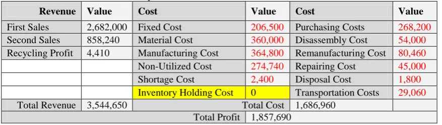
The effectiveness of the model has been verified through solving two examples with different demand patterns. Other parameters are assumed to be constant and having the values given in Table 2.

Table 2: Nominal values of the model parameters

Parameter Value Parameter Value

Virgin products prices 100, 150 and 200 Supplier locations fixed costs. 10,000 Weights of the three products 1, 2 and 3 Kg. Factory location fixed costs. 50,000 Manufacturing time of each product 1, 2 and 3 hr. Distributor locations fixed costs. 5,000 Remanufacturing time of each

product 2, 3 and 4 hr.

Disassembly location fixed

costs. 2,000

Second customer demand for each

product in each period 500

Redistribution location fixed

costs. 2,000

Second products price ratio 80 % Disposal location Fixed costs. 1,000 Returned products quality (may be

random) 20 % Supplier recycling capacity (kg) 2,000

Material cost per kilogram 10 Supplier capacity (kg) 4,000 Manufacturing costs per unit 10 Factory store capacity 2,000 Shortage cost for each product per

period 5, 10 and 15

Factory raw material storing

capacity (kg) 4,000

Non-Utilized manufacturing

capacity cost 10

Factory manufacturing capacity

(hours) 6,000

Non-Utilized remanufacturing

capacity cost 10

Factory remanufacturing

capacity (hours) 2,000 Factory holding cost 3 Distributor store capacity 4,000 Distributor holding cost 2 Disassembly location capacity 2,000 Disassembly cost per unit 3 Redistribution capacity 2,000 Recycling cost per unit 5 Disposal location capacity 1,000 Remanufacturing cost per unit 10 Max return ratio 50 %

Repairing cost 5 Repairing ratio 50%

Disposal cost 1 Recycling ratio 10%

Max number of operating suppliers, factories, distributors, disassembles and redistributors

3 Remanufacturing ratio 30%

Max number of first customers 4 Disposal ratio 10%

Max number of second customers 2 Batch sizes 1

4.1 EXAMPLE 1

4.1.1 EXAMPLE 1: INPUTS

The model has been verified through the following case study where the input parameters are considered as showing in Table 2. The demand patterns are assumed for all customers as shown in Table 3.

Table 3: Demand of each customer in each period for each product.

Required Demand

Period Customer 1 Customer 2 Customer 3 Customer 4

P1 P2 P3 P1 P2 P3 P1 P2 P3 P1 P2 P3

1 470 500 530 470 500 530 470 500 530 470 500 530

2 460 490 520 460 490 520 460 490 520 460 490 520

3 450 480 510 450 480 510 450 480 510 450 480 510

4.1.2 EXAMPLE 1: OUTPUTS AND DISCUSSION

The resulted optimal network is as shown in Figure 2.

(9)

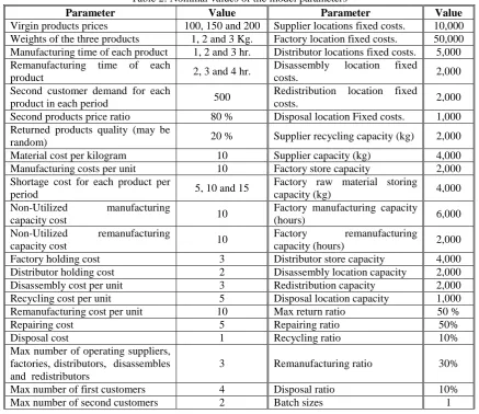
Total profit, total cost, total revenue, and their elements are given in Table 4. Only the Inventory Holding Cost equals zero which means that there is no inventory at all in the network.

Table 4: Total profit, total cost, total revenue, and their elements.

Revenue Value Cost Value Cost Value

First Sales 2,682,000 Fixed Cost 206,500 Purchasing Costs 268,200

Second Sales 858,240 Material Cost 360,000 Disassembly Cost 54,000

Recycling Profit 4,410 Manufacturing Cost 364,800 Remanufacturing Cost 80,460

Non-Utilized Cost 274,740 Repairing Cost 45,000

Shortage Cost 2,400 Disposal Cost 1,800

Inventory Holding Cost 0 Transportation Costs 29,060

Total Revenue 3,544,650 Total Cost 1,686,960

Total Profit 1,857,690

Where the quantities of batches transferred from suppliers to the factories and from factories to distributors are shown in Table 5. Flow balancing is noticed in Table 5 where the total weights of transferred materials are the same of 36000 kg.

Table 5: Number of batches transferred from suppliers and factories.

From Suppliers Factories

S1 S2 S3 F1 F2 F3

Period RM RM RM P1 P2 P3 P1 P2 P3 P1 P2 P3

1 4000 4000 4000 940 735 530 1 744 837 919 501 693

2 4000 4000 4000 460 990 520 460 120 1100 940 750 520

3 4000 4000 4000 900 785 510 347 775 701 553 480 829

Weight 12000 12000 12000 2300 5020 4680 808 3278 7914 2412 3462 6126

Total W. 36000 36000

The number of batches transferred from distributors to customers for all products in all period of also 36000 kg is shown in Table 6.

(10)

Given Quantities

P1 P2 P3 P1 P2 P3 P1 P2 P3 P1 P2 P3

1 470 500 530 470 490 470 470 490 530 450 500 530

2 460 490 520 460 500 580 460 380 520 480 490 520

3 450 480 510 450 480 510 450 600 510 450 480 510

Weight (Kg.) 1380 2940 4680 1380 2940 4680 1380 2940 4680 1380 2940 4680

Total Weights 36000

The shortage can be calculated easily by subtracting given quantities shown in Table 6 from the required quantities (demand) shown in Table 3 and it is shown in Table 7. Table 7 shows that all shortages are compensated in the next periods and these shortages resulted in a shortage cost of 2400 as shown in Table 4.

Table 7: Shortages.

Shortage per period

P1 P2 P3 P1 P2 P3 P1 P2 P3 P1 P2 P3

1 0 0 0 0 10 60 0 10 0 20 0 0

2 0 0 0 0 -10 -60 0 110 0 -20 0 0

3 0 0 0 0 0 0 0 -120 0 0 0 0

Weight (Kg.) 0 0 0 0 0 0 0 0 0 0 0 0

Total Weights 0

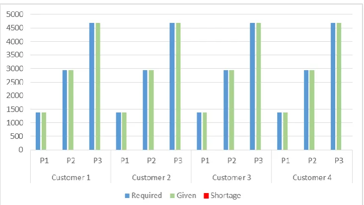
Figure 3 depicts the given quantities versus demand for all customer and all products. It can be noticed that they are all equal which means that there are no final shortages. Figure 4 shows that the total required weights are more than the network capacity in the first period equals it at the second period, and less than it at the third period which explains shortage compensation.

Figure 3: Given quantities versus demand for all customer and all products.

(11)

The flow in the reverse direction begins by receiving the returned products from the first customers by disassembly locations. Table 8 gives the maximum flow weights and the actual flow weights. It is noticed that the disassembly locations receives the maximum flow weights of 18000 kg. So, other actual weights of the repaired, recycled, remanufactured, disposed and redistributed equal the maximum flow weights. The number of products of 18000 kg weight purchased by disassembly locations from the first customers is shown in Table 9.

Table 8: Maximum and actual flow weights.

Ratio Max. flow weights Actual flow weights

Returned 0.5 18000 18000

Redistributed 0.8 14400 14400

Repaired 0.5 9000

18000

9000

18000

Recycled 0.1 1800 1800

Remanufactured 0.3 5400 5400

Disposed 0.1 1800 1800

Table 9: Number of products purchased by disassembly locations from the first customers.

Retuned Quantities

To A1 A2 A3

Period C1A1 C1A2 C1A3

P1 P2 P3 P1 P2 P3 P1 P2 P3

1 235 250 265 0 0 0 0 0 0

2 230 245 260 0 0 0 0 0 0

3 225 240 255 0 0 0 0 0 0

Period C2A1 C2A2 C2A3

P1 P2 P3 P1 P2 P3 P1 P2 P3

1 0 0 0 235 245 235 0 0 0

2 0 0 0 230 250 290 0 0 0

3 0 0 0 225 240 255 0 0 0

Period C3A1 C3A2 C3A3

P1 P2 P3 P1 P2 P3 P1 P2 P3

1 0 0 0 0 0 0 235 245 265

2 0 0 0 0 0 0 230 190 260

3 0 0 0 0 0 0 225 300 255

Period C4A1 C4A2 C4A3

P1 P2 P3 P1 P2 P3 P1 P2 P3

1 55 80 85 105 165 45 65 5 135

2 0 25 150 0 200 0 240 20 110

(12)

Weight (Kg.) 790 2000 3210 970 2360 2670 1000 1520 3480

Total Weights 18000

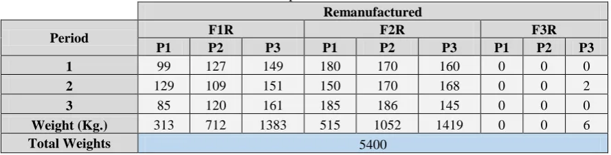
The number and weights of remanufactured, repaired, and delivered to the second customers matching Table 8 are presented in Tables 10, 11 and 12 respectively.

Table 10: Flow of remanufactured products from factories to redistributors.

Remanufactured

Period F1R F2R F3R

P1 P2 P3 P1 P2 P3 P1 P2 P3

1 99 127 149 180 170 160 0 0 0

2 129 109 151 150 170 168 0 0 2

3 85 120 161 185 186 145 0 0 0

Weight (Kg.) 313 712 1383 515 1052 1419 0 0 6

Table 11: Flow of repaired products from disassembly locations to redistributors.

Repaired

Period A1R A2R A3R

P1 P2 P3 P1 P2 P3 P1 P2 P3

1 145 165 175 170 205 140 150 125 200

2 115 135 205 115 225 145 235 105 185

3 135 200 155 200 160 160 115 150 195

Weight (Kg.) 395 1000 1605 485 1180 1335 500 760 1740

The number of batches transferred to the second customer through the reverse chain is shown in Table 12.

Table 12: Flow of refurbished products from redistributors to second customers.

Second Products

To K1 K2

Period R1K1 R1K2

P1 P2 P3 P1 P2 P3

1 244 292 324 0 0 0

2 244 244 356 0 0 0

3 220 320 316 0 0 0

Period R2K1 R2K2

P1 P2 P3 P1 P2 P3

1 0 0 0 350 375 300

2 0 0 0 265 395 313

3 0 0 0 385 346 305

Period R3K1 R3K2

P1 P2 P3 P1 P2 P3

1 0 0 0 150 125 200

2 0 0 0 235 105 187

3 0 0 0 115 150 195

Weight (Kg.) 708 1712 2988 1500 2992 4500

4.2 EXAMPLE 2

4.2.1 EXAMPLE 2: INPUTS

Demand patterns are assumed for all customers as shown in Table 13.

Table 13: Demand of each customer in each period for each product.

(13)

P1 P2 P3 P1 P2 P3 P1 P2 P3 P1 P2 P3

1 450 480 510 450 480 510 450 480 510 450 480 510

2 460 490 520 460 490 520 460 490 520 460 490 520

3 470 500 530 470 500 530 470 500 530 470 500 530

4.2.2 EXAMPLE 2: OUTPUTS AND DISCUSSION

The resulted optimal network is as shown in Figure 5.

Figure 5: The resulted optimal network of example 2.

Total profit, total cost, total revenue, and their elements are given in Table 14. Only the inventory holding cost equals zero which means that there is no inventory at all in the network.

Table 14: Total profit, total cost, total revenue, and their elements.

Revenue Value Cost Value Cost Value

First Sales 2,666,000 Fixed Cost 206,500 Purchasing Costs 266,600

Second Sales 853,120 Material Cost 357,600 Disassembly Cost 53,640

Recycling Profit 4,390 Manufacturing Cost 377,200 Remanufacturing Cost 79,980

Non-Utilized Cost 262,820 Repairing Cost 44,700

Shortage Cost 1,200 Disposal Cost 1,788

Inventory Holding Cost 0 Transportation Costs 28,589

Total Revenue 3,523,510 Total Cost 1,680,617

Total Profit 1,842,893

Where the quantities of batches transferred from suppliers to the factories and from factories to distributors are shown in Table 15. Flow balancing is noticed in Table 15 where the total weights of transferred materials are the same of 35760 kg.

Table 15: Number of batches transferred from suppliers and factories.

From Suppliers Factories

(14)

Period RM RM RM P1 P2 P3 P1 P2 P3 P1 P2 P3

1 3760 4000 4000 450 890 510 899 70 987 451 960 543

2 4000 4000 4000 920 490 700 0 710 860 920 760 520

3 4000 4000 4000 471 500 843 938 1000 354 471 500 843

Weight 11760 12000 12000 1841 3760 6159 1837 3560 6603 1842 4440 5718

Total W. 35760 35760

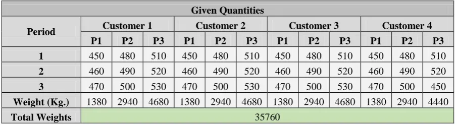
The number of batches transferred from distributors to customers for all products in all period of also 35760 kg is shown in Table 16

Table 16: Number of batches transferred from distributors to customers.

Given Quantities

P1 P2 P3 P1 P2 P3 P1 P2 P3 P1 P2 P3

1 450 480 510 450 480 510 450 480 510 450 480 510

2 460 490 520 460 490 520 460 490 520 460 490 520

3 470 500 530 470 500 530 470 500 530 470 500 450

Weight (Kg.) 1380 2940 4680 1380 2940 4680 1380 2940 4680 1380 2940 4440

The shortage can be calculated easily by subtracting given quantities shown in Table 16 from the required quantities (demand) shown in Table 13 and it is shown in Table 17. Table 17 shows that all shortages occurred only on the third product for the fourth (the furthest) customer because the network capacity is lower than the required as shown in Figure 7 and this shortage resulted in a shortage cost of 1200 as shown in Table 14.

Table 17: Shortages.

Shortage

P1 P2 P3 P1 P2 P3 P1 P2 P3 P1 P2 P3

1 0 0 0 0 0 0 0 0 0 0 0 0

2 0 0 0 0 0 0 0 0 0 0 0 0

3 0 0 0 0 0 0 0 0 0 0 0 80

Weight (Kg.) 0 0 0 0 0 0 0 0 0 0 0 240

Figure 6 depicts the given quantities versus demand for all customer and all products. It can be noticed that they are all not equal which means that there is a final shortage for customer 4 from product 3. Figure 7 shows that the total required weights is more than the network capacity in the third period, equals it at the second period, and less than it at the first period which explains final shortage.

(15)

Figure 7: Total required weights vs. network capacity

The flow in the reverse direction begins by receiving the returned products from the first customers by disassembly locations. Table 18 gives the maximum flow weights and the actual flow weights. It is noticed that the disassembly locations receives the maximum flow weights of 17880 kg. So, other actual weights of the repaired, recycled, remanufactured, disposed and redistributed equal the maximum flow weights. The number of products of 17880 kg weight purchased by disassembly locations from the first customers is shown in Table 19.

Table 18: Maximum and actual flow weights.

Ratio Max. flow weights Actual flow weights

Returned 0.5 17880 17880

Redistributed 0.8 14304 14304

Repaired 0.5 8940

17880

8940

17880

Recycled 0.1 1788 1788

Remanufactured 0.3 5364 5364

Disposed 0.1 1788 1788

Table 19: Number of products purchased by disassembly locations from the first customers.

Retuned Quantities

To A1 A2 A3

(16)

P1 P2 P3 P1 P2 P3 P1 P2 P3

1 225 240 255 0 0 0 0 0 0

2 230 245 260 0 0 0 0 0 0

3 235 250 265 0 0 0 0 0 0

Period C2A1 C2A2 C2A3

P1 P2 P3 P1 P2 P3 P1 P2 P3

1 0 0 0 225 240 255 0 0 0

2 0 0 0 230 245 260 0 0 0

3 0 0 0 235 250 265 0 0 0

Period C3A1 C3A2 C3A3

P1 P2 P3 P1 P2 P3 P1 P2 P3

1 0 0 0 0 0 0 225 240 255

2 0 0 0 0 0 0 230 245 260

3 0 0 0 0 0 0 235 250 265

Period C4A1 C4A2 C4A3

P1 P2 P3 P1 P2 P3 P1 P2 P3

1 5 90 115 5 60 135 215 90 5

2 0 85 110 230 135 0 0 25 150

3 15 100 85 215 0 85 5 150 55

Weight (Kg.) 710 2020 3270 1140 1860 3000 910 2000 2970

Total Weights 17880

The number and weights of remanufactured, repaired, and delivered to the second customers matching Table 18 are presented in Tables 20, 21 and 22 respectively.

Table 20: Flow of remanufactured products from factories to redistributors.

Remanufactured

Period F1R F2R F3R

P1 P2 P3 P1 P2 P3 P1 P2 P3

1 105 103 131 165 155 175 0 30 0

2 121 119 147 155 175 165 0 0 0

3 127 125 141 155 175 165 0 0 0

Weight (Kg.) 353 694 1257 475 1010 1515 0 60 0

Total Weights ₅₃₆₄

Table 21: Flow of repaired products from disassembly locations to redistributors.

Repaired

Period A1R A2R A3R

P1 P2 P3 P1 P2 P3 P1 P2 P3

1 115 165 185 115 150 195 220 165 130

2 115 165 185 230 190 130 115 135 205

3 125 175 175 225 125 175 120 200 160

Weight (Kg.) 355 1010 1635 570 930 1500 455 500 1485

(17)

Table 22: Flow of refurbished products from redistributors to second customers.

Second Products

To K1 K2

Period R1K1 R1K2

P1 P2 P3 P1 P2 P3

1 220 268 316 0 0 0

2 236 284 332 0 0 0

3 252 300 316 0 0 0

Period R2K1 R2K2

P1 P2 P3 P1 P2 P3

1 0 0 0 280 305 370

2 0 0 0 385 365 295

3 0 0 0 380 300 340

Period R3K1 R3K2

P1 P2 P3 P1 P2 P3

1 0 0 0 220 195 130

2 0 0 0 115 135 205

3 0 0 0 120 200 160

Weight (Kg.) 708 1704 2892 1500 3000 4500

V. CONCLUSION

From the previous study, the following conclusions can be derived:

1. The proposed model is successful in designing forward-reverse logistics networks while considering multi-product in multi-period with three echelons (suppliers, factories and distributors) in the forward direction and two echelons (disassemblies and re-distributors) in the reverse direction.

2. Quality level of the returned products, return rate, and others may be tackled as random value, but it is assumed as a deterministic to facilitate discussion.

3. This model can be developed easily to match a wide range of practical cases. It is recommended to:

4. Take the time value of money into consideration. 5. Tackle the robustness of environmental parameters.

6. Take the percent defective of each facility into consideration.

REFERENCES

[1] El-Sayed, M., Afia, N., & El-Kharbotly, A. (2010). A stochastic model for forward–reverse logistics network design under risk. Computers & Industrial Engineering, 58(3), 423-431.

[2] Hatefi, S. M., & Jolai, F. (2014). Robust and reliable forward–reverse logistics network design under demand uncertainty and facility disruptions. Applied Mathematical Modelling, 38(9), 2630-2647.

[3] Mutha, A., & Pokharel, S. (2009). Strategic network design for reverse logistics and remanufacturing using new and old product modules. Computers & Industrial Engineering, 56(1), 334-346.

[4] Pishvaee, M. S., Jolai, F., & Razmi, J. (2009). A stochastic optimization model for integrated forward/reverse logistics network design. Journal of Manufacturing Systems, 28(4), 107-114.

[5] Ramezani, M., Bashiri, M., & Tavakkoli-Moghaddam, R. (2013). A new multi-objective stochastic model for a forward/reverse logistic network design with responsiveness and quality level. Applied Mathematical Modelling, 37(1), 328-344.

[6] Salema, M. I. G., Póvoa, A. P. B., & Novais, A. Q. (2009). A strategic and tactical model for closed-loop supply chains. OR spectrum, 31(3), 573-599.

[7] Serdar E. T. & Al-Ashhab M. S. (2016). Supply Chain Network Design Optimization Model for Multi-period Multi-product. International Journal of Mechanical & Mechatronics Engineering IJMME-IJENS, 16(01), 122-140.