Bayesian online algorithms for learning in discrete Hidden Markov Models

VolumeX_{, Number}0X_{, XX}200X _pp.X–XX

BAYESIAN ONLINE ALGORITHMS FOR LEARNING IN DISCRETE HIDDEN MARKOV MODELS

Roberto C. Alamino

Neural Computing Research Group, Aston University Main Building, Birmingham, B7 4ET, United Kingdom

Nestor Caticha

Instituto de F´ısica, Universidade de S˜ao Paulo CP 66318, S˜ao Paulo, SP, CEP 05389-970, Brazil

(Communicated by the associate editor name)

Abstract. We propose and analyze two different Bayesian online algorithms for learning in discrete Hidden Markov Models and compare their performance with the already known Baldi-Chauvin Algorithm. Using the Kullback-Leibler divergence as a measure of generalization we draw learning curves in simplified situations for these algorithms and compare their performances.

1. Introduction. The unifying perspective of the Bayesian approach to machine learning allows the construction of efficient algorithms and sheds light on the char-acteristics they should have in order to attain such efficiency. In this paper we construct and characterize the performance of mean field online algorithms for dis-creteHidden Markov Models (HMM) [5, 9] derived from approximations to a fully Bayesian algorithm.

HMMs form a class of graphical models used to model the behavior of time series. They have a wide range of applications which includes speech recognition [9], DNA and protein analysis [3, 4] and econometrics [10].

Discrete HMMs are defined by an underlying Markov chain with hidden statesqt, t= 1, ..., T, in the setS={s1, s2, ..., sn}, initial probability vectorπi =P(q1=si) and transition matrix Aij(t) = P(qt+1 = sj|qt =si), with i, j = 1, .., n. At each time step, the stateqtemits a stateytin the setO={o1, ..., om}with a probability given by Biα(t) =P(yt=oα|qt=si), withi= 1, ..., nand α= 1, ..., m. When A andB do not depend on time the HMM is saidhomogeneous, this is a simplifying assumption, which is not needed for online learning.

Theobserved states ytof the HMM represent the observations of the time series, i.e., a time series from timet= 1 tot=T is represented by the observed sequence yT

1 ={y1, y2, ..., yT}. The unavailable orhidden states qtform the so calledhidden sequence qT

1 ={q1, q2, ..., qT}.

2000Mathematics Subject Classification. Primary: 68T05; Secondary: 60J20, 62F15.

Key words and phrases. HMM, online algorithm, generalization error, Bayesian algorithm. This work was supported mainly by FAPESP and partially by EVERGROW, IP no. 1935 in FP6 of the EU.

The parameters that define the HMM areπ,AandBwhich we denote compactly as ω = (π, A, B). The probability of observing a particular sequence yT

1 given parametersω is

P(y1T|ω) =

X

qT

1

P(yT1, q

T 1|ω)

=X qT

1

P(y1)P(y1|q1)

T Y

t=2

P(qt+1|qt)P(yt|qt).

(1)

Most applications consist in adapting the parameters of the HMM in order to produce sequences which mimic the behavior of some given time series. This is the learning process on the HMM. Depending on how the data is presented it can range from offline toonline. In the former, the whole dataset, usually given by just one observed sequence yT

1, is presented to the algorithm and the optimal parameters are calculated all at once. In the later, the dataset, usually composed of a certain numberP of independently generated observed sequences, is presented only a part at a time after which, a partial calculation of the parameters is made. We will concentrate our analysis in the last case.

Several merit figures can be used to measure the performance of a learning al-gorithm. For the sake of simplicity we will study a scenario where the data set has been generated by a HMM of unknown parameters. This is an extension of the student-teacher scenario where the statistical mechanical properties of neural networks have been extensively studied. The performance of the learning process, as a function of the number of observations P, is given by how far, as measured by some suitable defined criterion, lies the student HMM from the teacher HMM. In this paper we only concentrate in the naturally arisingKullback-Leibler diver-gence (KL-divergence), which although not immediately usable in practice, since it needs knowledge from the unavailable teacher, is a simple extension of the idea of generalization error and therefore can be very informative.

We propose two algorithms for learning on HMMs and compare their perfor-mances with the online Baldi-Chauvin Algorithm (BC) [2] where a softmax repre-sentation of the HMM parameters is used to calculate a maximum likelihood esti-mate. Starting from a Bayesian formulation of the learning problem we introduce a Bayesian Online Algorithm (BOnA) for HMMs. This can be simplified, without noticeable deterioration of the performance, leading to aMean Posterior Algorithm (MPA). Using the KL-divergence, we draw learning curves for these algorithms in simplified situations and compare with the BC algorithm.

These methods, inspired by the works of Opper [7] and Amari [1] are essentially mean field methods [8]. The Bayesian prescription for the posterior usually leads to a distribution that cannot be handled in practice. The idea is to introduce a manifold of tractable distributions which will be used as priors. The information of the new datum leads, through Bayes theorem, to a non-tractable posterior. The basic inference step is to consider as the new prior to be used with the next datum, not the posterior itself, but one of the tractable distributions. Which one? The closest, in some sense. The choice of distance defines the algorithm.

2. The Bayesian Online Algorithm. The Bayesian Online Algorithm (BOnA), which can be found in [7], is a method for estimating parameters using the power of Bayesian inference.

Our task here is to adjust the HMM parameters ω using the information con-tained in a dataset given by

DP ={y1, ..., yP}. (2) To accomplish it in a Bayesian way, we need to estimate the parameters us-ing a probability distribution P(ω|DP) which encodes the information about the probability of the parameters after the observation ofDP. Assuming that the ob-servations inDP are independent, at each new sequence we can update our previous distribution in a new posterior using Bayes’ theorem.

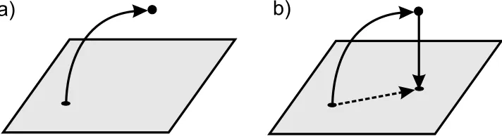
Figure 1. _{In gray we show the manifold of the tractable}

distri-butions. The two-step algorithm is represented by the arrows: a) 1st. step: a new observation modifies the former distribution tak-ing it away from the parametric family manifold. b) 2nd. step: the modified distribution is projected back into the original manifold by minimization of the KL-divergence.

If we choose a prior distribution belonging to a parametric family with parameters λ, after one update the posterior will no longer be in this family. The method consists in projecting this posterior back into the parametric manifold by minimizing the KL-divergence

DKL(P(ω|λP, yP+1)||P(ω|λP+1)) = Z

P(ω|λP, yP+1) lnP(ω|λ

P_{, y}P+1₎

P(ω|λP+1₎ dω, (3)

what is represented schematically in figure 1.

At each point in the learning process, the estimative for ω that we will choose will be its mean in the final distribution.

The choice of the parametric family of distributions will be dictated by the par-ticular problem we are dealing with. When the parametric family is of the form

P(x) = 1 Ze

−P

iλifi(x)_{, (4)}

which is the case when the distribution is obtained by the maximum entropy method using as constraints the average value ofnarbitrary functions fi(x)

hfi(x)iP ≡

Z

minimizing the KL-divergence turns out to be equivalent to equate the average of thenconstraint functions

hfjiP =hfjiQ, (6)

where the indices indicate in which distribution we need to take the averages and Q(x) is the still unprojected posterior.

2.1. Bayesian Online Algorithm for HMMs. In order to apply the BOnA to the case of HMMs, we need to choose an appropriate parametric family. Making the simplifying assumption that matricesπ,AandBare independent, we can write a factorized distribution

P(ω|u)≡ P(π|ρ)P(A|a)P(B|b), (7)

whereu= (ρ, a, b) are parameters of the distributions. The vectorπand each row of the matricesAandB are discrete probability distributions for the initial states, the transition of a given hidden state and the emission of an observed state by a given hidden one respectively. As they are different distributions, we will assume that they can be treated independently and factorize the distribution (7) once again using

P(A|a) =

n Y

i=1

P(Ai_|ai_{), P(B|b) =}

n Y

i=1

P(Bi_|bi_{), (8)}

where

Ai ≡(Ai1, ..., Ain), Bi≡(Bi1, ..., Bim), (9) which gives for (7)

P(ω|u)≡ P(π|ρ)

n Y

i=1

P(Ai_|ai_)P(Bi_|bi_{). (10)}

where each factor is a density of probability that a probability has a given value. A natural choice is the family of Dirichlet distributions

D(x|u) =_QNΓ(u0) i=1Γ(ui)

N Y

i=1 xui−1

i , (11)

where x= (x1, ..., xN) is a N-dimensional real vector andu= (u1, ..., uN) subject to the constraints

0≤xi≤1, N X

i=1

xi= 1, ui>0, (12)

andu0=P iui.

As (10) is a factorized distribution, the minimization of the KL-divergence can be made separately for each factor distribution. The Dirichlet distribution can be obtained from the maximum entropy method using as constraints the values of the averages of the logarithms of the variables [11]

0≤xi≤1, X

i

xi= 1, (13)

and

Z

dµD(x) = 1,

Z

wheredµis defined as

dµ≡δ X i

xi−1 !

Y

i

θ(xi)dxi. (15)

Extremizing the entropy subject to the constraints is equivalent to extremizing

L=

Z

dµDlnD+λ

Z

dµD −1

+X i

λi Z

dµDlnxi−αi

, (16)

and applyingδL/δD= 0 we have

δ X

i xi−1

! " Y

i θ(xi)

#

1 + lnD+λ+X i

λilnxi !

= 0, (17)

with solution

D(x) = exp(−λ−1)Y i

x−λi

i , (18)

which is the Dirichlet distribution forZ= exp(λ+ 1) and ui= 1−λi.

So, the minimization of the KL-divergence corresponds to equating the average of the logarithms in the original and projected distributions. The final result is

ψ(ρi)−ψ   X j ρj 

=hlnπii_Q≡µi(ρ), (19)

ψ(aij)−ψ X

k aik

!

=hlnAiji_Q≡µij(a),

ψ(biα)−ψ   X β biβ 

=hlnBiαi_Q≡µiα(b),

whereQis the posterior distribution andψis the digamma function, the logarithm derivative of the gamma function

ψ(x) = d

dxln Γ(x) = Γ0_(x)

Γ(x). (20)

We will call a set ofN equations of the form

ψ(xi)−ψ   X j xj 

=µi, (21)

withi= 1, ...N a digamma system in the variablesxi with coefficientsµi.

To solve the problem we need two more steps: calculate the coefficients µ and solve the digamma system (19).

Let us callPp_{(ω) the projected distribution after observation of the sequencey}p_, andQp+1_{(ω) the posterior distribution (not projected yet) after the observation of} the sequenceyp+1_{. Then, by Bayes’ theorem,}

Qp+1(ω) = 1 ZQ

Pp(ω)X qp+1

P(yp+1, qp+1|ω), (22)

ZQ= X

qp+1 Z

Due to the summation over hidden states, the posterior distribution is a mixture of Dirichlets. If we had access to these states, the posterior would be a simple Dirichlet distribution and we would not need the projection step. The projected distributionPp _{is, by construction, the product distribution}

Pp_{(ω) =P(π|ρ}p_)P(A|ap_)P(B|bp_{), (24)}

where ρp_{, a}p _{and b}p _{are the values of the parametersu after observation of the} sequenceyp_{. From here on, let us suppress the indices relative to the sequences by} adopting the convention that primed variables correspond to the upper indexp+ 1 and unprimed top. Then, equation (22) can be written as

Q0_{(ω) =} 1

ZQ0

P(π|ρ)P(A|a)P(B|b)X

q0

P(y0_{, q}0_{|π, A, B), (25)}

ZQ0 = X

q0 Z

dπ dA dBP(π|ρ)P(A|a)P(B|b)P(y0_{, q}0_{|π, A, B). (26)}

Using the notation

q0

t=si⇒π(qt0)≡πi, (27)

q0

t=si, q0t+1 =sj ⇒A(qt0, qt0+1)≡Aij, q0

t=si, y0t=oα⇒B(qt0, y0t)≡Biα, the normalization of the posterior can be factored as

ZQ0 = X

q0 Z

dπP(π|ρ)π(q0

1)·

Z

dAP(A|a) T0

−1

Y

t=1 A(q0

t, qt0+1)

× Z

dBP(B|b) T0 Y

t=1 B(q0

t, yt0),

(28)

whereT0 _{is the length of the sequencey}0_≡yp+1_{. The integrals onAandBcan be} factored once more in the rows of these matrices:

ZQ0 = X

q0 Z

dπP(π|ρ)π(q0

1)·

Y

i Z

dAi_P(Ai_|ai₎ Y q0

t=si

A(q0

t, q0t+1)

×Y

i Z

dBi_P(Bi_|bi₎ Y q0

t=si

B(q0

t, y0t).

(29)

The calculation of theµcoefficients in (19) now involves expectations over Dirich-let distributions of the form

µi=

*

 Y

j xrj

j 

lnxi +

. (30)

Taking the average over the Dirichlet distributionD(x|u), we have

µi= *

Y

j xrj

j +

[ψ(ui+ri)−ψ(u0+r0)], (31)

with

* Y

j xrj

j +

= QΓ(u0) jΓ(uj)

Q

jΓ(uj+rj)

solving the problem of calculating the coefficients of the digamma systems.

2.1.1. Digamma Systems. The next step is to solve the digamma systems them-selves. In order to find a solution for the general form

ψ(xi)−ψ 

 X

j xj



=µi, i= 1, ..., d, (33)

we devised the simple method of transforming these equations in a one-dimensional map and find numerically the fixed point by iterating from an arbitrary initial point. What we need to do is to solve forxi

xi=ψ−1 

µi+ψ 

 X

j xj



 

. (34)

Summation overiusing the definitionx0≡P

ixi gives

x0=X i

ψ−1_[µ

i+ψ(x0)]. (35)

We solve this equation by iteration of the map

x(0n+1)=

X

i

ψ−1_[µ i+ψ(x

(n)

0 )]. (36)

This completes the algorithm. BOnA suffers from a common problem of Bayesian algorithms: we have to sum over the hidden variables making the complexity scales asnT_{, i.e., exponential in the length of the observed sequences. In the BOnA case} we have a worse situation due to the great quantity of digamma functions needed to be calculated numerically. Everything summed up makes the algorithm very time consuming. In the next section, we will develop an approximation that runs faster, although still have exponential complexity in T. This is however not a problem since T can be kept fixed and small without depending on the total number of examples, this dependence must be stressed is polynomial.

2.2. Mean Posterior Approximation. The algorithm we present now will be called the Mean Posterior Approximation (MPA) and it is a simplification of the BOnA that is itself inspired in the results of its application to Gaussian distribu-tions.

With a hat over variables indicating the new estimated values, the matching of the means is given by

ˆ

πi=hπii_Q0 ⇒ρˆi=hπiiQ0 X

j ˆ

ρj, (37)

ˆ

Aij =hAiji_Q0 ⇒aˆij =hAijiQ0 X

k ˆ aik,

ˆ

Biα=hBiαi_Q0 ⇒ˆbiα=hBiαiQ0 X

β ˆ_biβ.

We still have some freedom that can be fixed by matching the first variance of each Dirichlet distribution. For the initial probabilitiesπ, defining ρ0≡P

iρi, this will be given by

π21

Q0 − hπ1i

2 Q0 =

ˆ

ρ1(ˆρ0−ρ1)ˆ ˆ

ρ2

0(ˆρ0+ 1)

. (38)

After some algebra we find that the final update equations for the parameters are

ˆ

ρi = hπiiQ0

hπ1iQ0−

π2 1

Q0

hπ2

1iQ0 − hπ1i

2 Q0

, (39)

ˆ

aij = haijiQ0

hai1iQ0−

a2 i1

Q0

ha2

i1iQ0 − hai1i

2 Q0

,

ˆ

biα = hbiαiQ0

hbi1iQ0 −

b2 i1

Q0

hb2

i1iQ0− hbi1i

2 Q0

.

1 10 100

p 0.1

d (Kullback-Leibler)

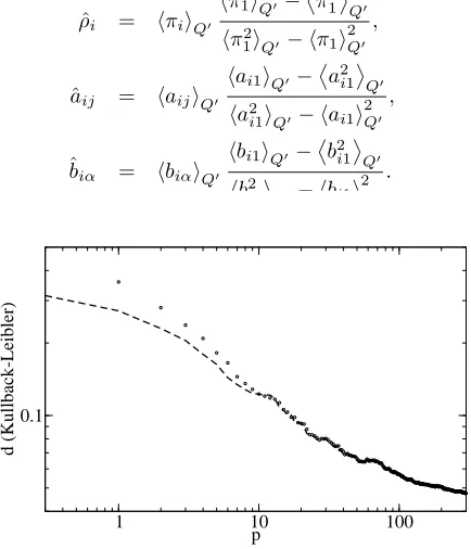
Figure 2. _{Comparison between the learning curves of MPA}

(dashed line) and BOnA (circles). Logarithmic scale.

The real computational time for BOnA was 340 minutes, while for MPA was 5 seconds in a 1GHz processor.

10 100 1000 10000

p 0.1

d (Kullback-Leibler)

0.001 0.01

0.1

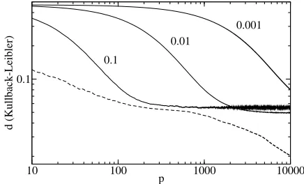
Figure 3. _{Comparison between MPA (dashed line) and}

Baldi-Chauvin (continuous lines). The values next to the curves indicate λfor the corresponding simulation. The learning rate was fixed to ηBC = 0.5. Logarithmic scale.

Figure 3 compares the performance of MPA to Baldi-Chauvin showing that the generalization ability of MPA is superior. The parameters of the simulations are n= 2,m= 3 andT = 2. The curves are the result of the average over 500 random teachers with symmetric initial students.

3. Conclusions. We proposed and analyzed two Bayesian algorithms for online learning in discrete HMMs: the full Bayesian Online Algorithm (BOnA) and the Mean Posterior Approximation (MPA) to the BOnA.

After introducing the BOnA, we developed a simplification that runs faster which we called MPA. The MPA was then compared with the Baldi-Chauvin algorithm and shown to perform better with respect to the generalization ability. Although MPA scales exponentially with the size of the sequence like BOnA, it is not a problem for we can fix this size to some small value and still have a good generalization.

We have applied these algorithms to learning real data time series with good preliminary results. We have also studied the effects of drifting rules and of sharp changes in the series. These results will be published elsewhere.

Acknowledgements. In addition to the funding cited in the beginning of this paper, we would like to thank also Evaldo Oliveira, Manfred Opper and Lehel Csato. This work was made mostly in the University of S˜ao Paulo, Brazil and part in Aston University, UK. We would also like to thank Prof. Ruedi Stoop for the kind invitation for contributing with this work.

REFERENCES

[1] S. Amari, Neural learning in structured parameter spaces - natural Riemannian gradient

NIPS’969, MIT Press (1996).

[2] P. Baldi and Y. ChauvinSmooth on-line learning algorithms for hidden Markov modelsNeural Computation6(1994), 307–318.

[4] R. Durbin, S. Eddy, A. Krogh and Mitchison, G. “Biological Sequence Analysis: Probabilistic Models of Proteins and Nucleic Acids” Cambridge University Press, Cambridge, 1998. [5] Y. Ephraim and N. MerhavHidden Markov processes IEEE Trans. Inf. Theory48(2002),

1518–1569.

[6] T. Heskes and W. Wiegerinck On-line learning with time-correlated examples in “On-line Learning in Neural Networks” (Ed. D. Saad), Cambridge University Press, Cambridge, (1998), 251–278.

[7] M. OpperA Bayesian approach to on-line learningin “On-line Learning in Neural Networks” (Ed. D. Saad), Publications of the Newton Institute, Cambridge Press, Cambridge, (1998), 363–378.

[8] M. Opper and D. Saad “Advanced Mean Field Methods: Theory and Practice” The MIT Press, 2001.

[9] L. R. RabinerA tutorial on hidden Markov models and selected applications in speech recog-nition Proc. IEEE77(1989), 257–286.

[10] T. Ryd´en, T. Terasvirta and S. AsbrinkStylized facts of daily return series and the hidden Markov model J. Applied Econometrics13(1998), 217-244.

[11] M. O. Vlad, M. Tsuchiya, P. Oefner and J. Ross Bayesian analysis of systems with ran-dom chemical composition: renormalization-group approach to Dirichlet distributions and the statistical theory of dilution Phys. Rev. E65(2001), 011112(1)–01112(8).

Received September 2006; revised February 2007.