Online Bayesian Learning in Probabilistic Graphical Models using Moment Matching with Applications

(1)

Online Bayesian Learning in

Probabilistic Graphical Models using

Moment Matching with Applications

by

Farheen Omar

A thesis

presented to the University of Waterloo in fulfillment of the

thesis requirement for the degree of Doctor of Philosophy

in

Computer Science

Waterloo, Ontario, Canada, 2016

c

(2)

I hereby declare that I am the sole author of this thesis. This is a true copy of the thesis, including any required final revisions, as accepted by my examiners.

(3)

Abstract

Probabilistic Graphical Models are often used to efficiently encode uncertainty in real world problems as probability distributions. Bayesian learning allows us to compute a posterior distribution over the parameters of these distributions based on observed data. One of the main challenges in Bayesian learning is that the posterior distribution can become exponentially complex as new data becomes available. Secondly, many algorithms require all the data to be present in memory before the parameters can be learned and may require retraining when new data becomes available. This is problematic for big data and expensive for streaming applications where new data arrives constantly.

In this work I have proposed an online moment matching algorithm for Bayesian learn-ing called Bayesian Moment Matchlearn-ing (BMM). This algorithm is based on Assumed Den-sity Filtering (ADF) and allows us to update the posterior in a constant amount of time as new data arrives. In BMM, after new data is received, the exact posterior is projected onto a family of distributions indexed by a set of parameters. This projection is accomplished by matching the moments of this approximate posterior with those of the exact one. This allows us to update the posterior at each step in constant time. The effectiveness of this technique has been demonstrated on two real world problems.

Topic Modelling: Latent Dirichlet Allocation (LDA) is a statistical topic model that examines a set of documents and based on the statistics of the words in each document, discovers what is the distribution over topics for each document.

Activity Recognition: Tung et al [29] have developed an instrumented rolling walker with sensors and cameras to autonomously monitor the user outside the laboratory setting. I have developed automated techniques to identify the activities performed by users with respect to the walker (e.g.,walking, standing, turning) using a Bayesian network called Hidden Markov Model. This problem is significant for applied health scientists who are studying the effectiveness of walkers to prevent falls.

My main contributions in this work are:

• In this work, I have given a novel interpretation of moment matching by showing that there exists a set of initial distributions (different from the prior) for which exact Bayesian learning yields the same first and second order moments in the posterior as moment matching. Hence the Bayesian Moment matching algorithm is exact with respect to an implicit posterior.

(4)

• Label switching is a problem which arises in unsupervised learning because labels can be assigned to hidden variables in a Hidden Markov Model in all possible permuta-tions without changing the model. I also show that even though the exact posterior hasn! components each corresponding to a permutation of the hidden states, moment matching for a slightly different distribution can allow us to compute the moments without enumerating all the permutations.

• In traditional ADF, the approximate posterior at every time step is constructed by minimizing KL divergence between the approximate and exact posterior. In case the prior is from the exponential family, this boils down to matching the ”natural” moments. This can lead to a time complexity which is the order of the number of variables in the problem at every time step. This can become problematic particularly in LDA, where the number of variables is of the order of the dictionary size which can be very large. I have derived an algorithm for moment matching called Linear Moment Matching which updates all the moments in O(n) wheren is the number of hidden states.

• I have derived a Bayesian Moment Matching algorithm (BMM) for LDA and com-pared the performance of BMM against existing techniques for topic modelling using multiple real world data sets.

• I have developed a model for activity recognition using Hidden Markov Models (HMMs). I also analyse existing parameter learning techniques for HMMs in terms of accuracy. The accuracy of the generative HMM model is also compared to that of a discriminative CRF model.

• I have also derived a Bayesian Moment Matching algorithm for Activity Recognition. The effectiveness of this algorithm on learning model parameters is analysed using two experiments conducted with real patients and a control group of walker users.

(5)

Acknowledgements

Pascal Poupart was my supervisor during my research on this thesis. He guided and challenged me throughout my research by forcing me to approach my research with crystal clarity and focus. He was thoroughly engaged with my work and was always available whenever I needed assistance and feedback. He always worked with me to untangle each roadblock that I encountered. Even after I had a baby and was working remotely to-wards the end, his support never flagged. I am truly indebted to him for his mentoring, supervision and kind understanding and patience.

I am also grateful to my thesis committee: Dan Lizzotte and Jesse Hoey for their critical analysis of my work, John Zelek who gave me an engineering perspective on how this work can be utilized and Richard Zemel my external examiner who gave me wonderful insights on how to polish this research further and suggesting future directions. I would also like to thank Han Zhao, Mathieu Sinn and Jakub Truszkowski for contributing to this research.

Margaret Towell in the Computer Science Grad office has always been an invaluable resource who was untiring in her readiness to assist students whenever any help was needed in the catacombs of paperwork.

My husband Omar has been instrumental in helping me become who I am today. He has given me courage and support and also served as a good sounding board for my ideas. He also gave me great critical insights on my work. Above all he convinced me that I could accomplish all I dream of even when I had grown up with a mindset that discouraged achievement for women.

I would also like to give a shout out to my mother-in-law Mrs Ghazala Yawar who provided me with a support system without which I would not have been able to do justice to my young child and my research. I want to thank my mother Neelofur Shahid who is the kindest being that I know. Her support throughout my early education and university and her kindness as a parent is the reason why I am here today. I want to thank my father who despite being the biggest source of challenges in my life, inculcated a thirst of knowledge, reading and planted the seeds of inquisitiveness in me that have led me to pursue research professionally. I would also like to thank my brother Salman Shahid for being a partner in crime when I was younger and a source of support even now. A special thanks to my brother-in-law Awais Zia Khan who was always ready to babysit and offer other help when needed. And lastly a big thanks to my little boy Rohail who is the most wonderful of children. If he were not the sweet person that he is I would not have been able to complete what I had started.

(6)

Dedication

(7)

List of Tables

5.1 Summary Statistics of the data sets . . . 57

5.2 Time taken in seconds by each algorithm to go over complete data. . . 63

6.1 Activities performed in Experiment 1 . . . 67

6.2 Additional activities performed during Experiment 2 . . . 68

6.3 Highest value for each sensorswith respect to activityy, arg maxePr (es|y). The second row for each activity is the probability of this highest value maxePr (es|y). This table is based on the data from the second experiment 70 6.4 Empirical Transition Distribution for Experiment 2 . . . 71

6.5 Confusion matrix for HMM model Experiment 1 activities using load sensor values. Observation model learned from data. Activity persistence probabil-ity τ = 4000. Prediction using Filtering. Window size is 25. Features used are Accelerometer Measurements, Speed, Load cell values. Overall accuracy is 91.1%. . . 82

6.6 Confusion matrix for HMM model for Experiment 1 using center of pres-sure. Observation model learned from data. Activity persistence parameter: τ = 4000. Prediction using Filtering. Window size is 25. Features used are Accelerometer Measurements, Speed, Frontal plane COP, Saggital plane COP and total weight. Overall accuracy is 88%. . . 83

6.7 Confusion matrix for CRF model for Experiment 1 data using center of pres-sure. Window size is 25. Features used are Accelerometer Measurements, Speed, Frontal plane COP, Saggital plane COP and Total Weight. Overall accuracy is 93.8%. . . 83

(12)

6.8 Confusion matrix for HMM model for Experiment 2 data using load sensor values. Observation model learned from data. activity persistence probabil-ity τ = 4000. Prediction using Filtering. Window size is 25. Features used are Accelerometer Measurements, Speed, load cell values. Overall accuracy is 79.1%. . . 84

6.9 Confusion matrix for HMM model for for Experiment 2 data using center of pressure. Observation model learned from data. activity persistence prob-ability τ = 4000. Prediction using Filtering. Window size is 25. Features used are Frontal plane COP, Saggital plane COP and total weight. Overall accuracy is 77.2%. . . 84

6.10 Confusion matrix for CRF model for Experiment 2 data using center of pres-sure. Window size is 25. Features used are Accelerometer Measurements, Speed, Frontal plane COP, Saggital plane COP and total weight. Overall accuracy is 80.8%. . . 85

6.11 Confusion matrix for HMM model results for Experiment 2 data using nor-malized load sensor values. Observation model and transition model learned from data. Prediction using Filtering. Window size is 25. Features used are Accelerometer Measuremens, Speed, Normalized load cell values. Overall accuracy is 80.8%. . . 85

6.12 Experiment 1 percentage accuracy for each activity. COP implies that center of pressure feature is used instead of load cell values. Prediction is done using the Forward-Backward Algorithm . . . 86

6.13 Experiment 2 percentage accuracy for each activity. NL means the normal-ized load values are used. COP implies that center of pessure feature is used instead of normalized load values. . . 87

7.1 Moment Matching results for Experiment 1 data using center of pressure. Window size is 25. Features used are Accelerometer Measurements, Speed, Frontal plane COP, Saggital plane COP and Total Weight. Overall accuracy is 76.2%. . . 104

7.2 Experiment 1 percentage accuracy for each activity for unsupervised learning techniques. Prediction is done using the Forward-Backward Algorithm . . 105

7.3 Experiment 2 percentage accuracy for each activity. NL means the normal-ized load values are used. COP implies that center of pessure feature is used instead of normalized load values. . . 105

(13)

(14)

List of Figures

1.1 The instrumented walker developed by [73] et. al. The walker has a 3-D accelerometer, 4 load cells, 1 wheel encoder and 2 cameras . . . 7

2.1 Latent Dirichlet Allocation Topic Model . . . 16

2.2 A Bayesian Hidden Markov Model. . . 20

4.1 Expectation ofθwith respect to the approximate posterior vs. the number of observations. Q(θ) is the approximate posterior learnt by matching Mlog(θ)

where as Q0(θ) is the approximate posterior learnt by matching M(θ). The

true value of θ used to generate the observations is 0.7. . . 38

5.1 Latent Dirichlet Allocation Topic Model . . . 40

5.2 Comparison of different learning algorithms for topic modeling for the NIPS dataset. The number of topics T = 25. The second figure is the perplexity for vblp, gs and bplp zoomed . . . 58

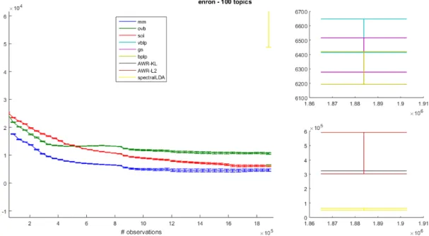
5.3 Comparison of different learning algorithms for topic modeling for the En-ron dataset. The number of topics T = 100. The top right figure is the perplexity of vblp, gs and bplp and the bottom right is the preplexity of AWR-KL, AWR-L2 and Spectral LDA . . . 59

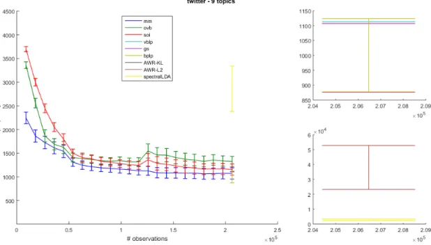
5.4 Comparison of different learning algorithms for topic modeling for the Twit-ter dataset. The number of topicsT = 9. The top right figure is the perplex-ity of vblp, gs and bplp and the bottom right is the preplexperplex-ity of AWR-KL, AWR-L2 and Spectral LDA . . . 60

5.5 Comparison of different learning algorithms for topic modeling for the NY-Times dataset. The number of topics T = 100. . . 61

(15)

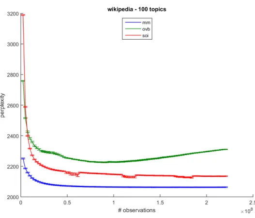
5.6 Comparison of different learning algorithms for topic modeling for the Wikipedia dataset. The number of topics T = 100. . . 62

5.7 Comparison of different learning algorithms for topic modeling for the PubMed dataset. The number of topics T = 100. . . 63

5.8 EP vs MM on synthetic data. T = 5 . . . 64

6.1 Course for data collection experiment done with the walker. Healthy young subjects were asked to follow this course . . . 66

6.2 Course used in data collection experiment for older subjects who are walker users . . . 67

6.3 A Hidden Markov Model For Activity Recognition . . . 72

6.4 A Hidden Markov Model For Activity Recognition with Bayesian Priors . . 73

6.5 Accuracy, Precision and Recall for various algorithms in each experiment. . 86

7.1 A Hidden Markov Model For Activity Recognition with Bayesian Priors . . 91

7.2 Accuracy, Precision and Recall for various algorithms in each experiment. . 106

7.3 Accuracy, Precision and Recall for Online EM and Moment Matching on synthetic data. . . 107

(16)

Chapter 1

Introduction

Probability theory allows us to capture inherent uncertainty that arises in real world pro-cesses. This uncertainty may stem from the fact that some parts of the process are not observable directly or because we are trying to predict the values of future events based on observations in the past. The probability of an event can be informally defined as the degree of belief that this event will happen. A probability distribution is a function that assigns a real numberP r(X =x) to a random variableX which represents the degree of belief that

X will take value x. In some cases, the distribution has the form Pr (X =x|θ) =f(x, θ).

θ is called the parameter of the distribution. Probabilistic Graphical Models allow us to encode probability distributions over high dimensional event spaces efficiently. One of the key tasks in constructing these models is to learn the value of parameters of each distribu-tion that best describe the observed data. Bayesian learning provides a paradigm which allows us to compute a posterior belief about model parameters, based on a prior belief about their values and observed data. This posterior belief is usually encoded in the form of a posterior distribution over the model parameters.

One of the main challenges in Bayesian learning is that the posterior distribution can become very complex as new information becomes available. In some cases, the posterior can be an exponentially large mixture of distributions. Hence representing the posterior and calculating its statistics can be computationally expensive. Typically algorithms aim to construct an approximate posterior either by minimizing some distance metric between the exact and approximate posterior, or by drawing samples from the exact posterior. Most of these algorithms require the complete data to be present in the memory at the time of learning and usually require the model to be retrained if new data arrives. More recently, online versions of some of these algorithms have been developed that are able to incorporate new information without retraining the complete model. These online techniques use a

(17)

sample set of the data known as a mini-batch to update the parameters such that some distance metric is minimized.

Maximum Likelihood Learning is an alternative to Bayesian Learning where instead of computing a posterior distribution over the parameters, we compute point estimates for the values of parameters that maximize the likelihood of the observed data. This often involves solving a non convex optimization problem and the algorithms are prone to get stuck in local optima.

Another class of algorithms including Assumed Density Filtering, Expectation Propa-gation [56] and the online algorithm described in [5] project the complex exact posterior onto a simpler family of distributions indexed by a set of parameters. This projection is done by minimizing the a distance measure between the exact posterior and a member of this family of distributions.

In this work I have explored and extended the concepts central to assumed density filtering by concentrating on the moment matching framework of the algorithm and propose efficient extensions to it. I also give a novel interpretation of this procedure that allows it to be viewed as an exact inference technique instead of an approximate one.

1.1

Moment Matching

In many applications, Bayesian learning can be intractable since the posterior becomes an exponentially large mixture of products of Dirichlets. However, the full posterior is rarely used in practice. A few moments (i.e, mean and variance) are often sufficient to estimate the parameters with some form of confidence.

I have proposed a moment matching technique called Bayesian Moment Matching (BMM) which is based on Assumed Density Filtering. In Bayesian Moment Matching, at every time step, the exact posterior is projected onto a family of distributions indexed by a set of parameters. Given a prior that belongs to this family of distributions; after every observation is received, the exact posterior is computed through a Bayesian update. Then this exact posterior is again projected onto the same family as the initial prior dis-tribution such that some of the moments of the exact posterior are equal to those of the approximate posterior. This allows us to compute all the parameters required to specify the posterior. The moment matching can be done by solving a linear system of equations which can be solved analytically.

(18)

Exact Learning w.r.t. an Implied Prior

In Assumed Density Filtering, the primary objective is to find a target distribution in a family of distributions such that the distance between this target distribution and the exact posterior is minimized. This minimization leads to matching of some moments of the exact and approximate posteriors. Given that the observations are informative (i.e. help us distinguish between hidden states), after seeing a very large number of observations, most of the weight of the posterior will be concentrated at one point which will correspond to the first order moment of the posterior (or mean) at that time step. Therefore, in the Bayesian moment matching algorithm proposed in this thesis, we match the first and second order raw moments of the posterior. I have also presented a novel motivation for this moment matching procedure by showing that there exists a set of initial distributions (different from the prior) for which exact Bayesian learning yields the same first and second order moments in the posterior as moment matching. My approach exploits the fact that a small set of moments of the prior need to be specified before any data is observed. After receiving each observation, moment matching allows us to set moments of the posterior. We can solve multiple systems of equations that use the posterior moments to implicitly specify higher order moments in the prior. Hence, the algorithm incrementally specifies the moments of the prior as they become needed in the computation. If we start with this implied prior and perform exact moment matching, then the first order moments of the posterior will be the same as those of the posterior acquired by moment matching. Therefore the overall computation is exact with respect to this prior. To our knowledge, this algorithm is the first Bayesian learning technique that can process each additional word in a constant amount of time and is exact with respect to an implied prior.

I have demonstrated the effectiveness of this technique on two real world problems.

1.2

Topic Modeling

In natural language processing statistical topic models are constructed to discover the abstract topics that occur in a collection of documents. A document typically concerns multiple topics in different proportions. A topic model captures this intuition as a statis-tical model that examines a set of documents and based on the statistics of the words in each document, discovers what the topics might be and what is the balance of topics for each document. These topics can be used to cluster and organize the corpus. The main computational problem is to infer the conditional distribution of these variables given an observed set of documents [54]. The exact posterior in LDA is an exponentially large

(19)

mixture of products of Dirichlets. Hence exact inference and parameter learning can be challenging.

Algorithms for topic modeling attempt to construct approximations to the exact pos-terior either by minimizing some distance metric or by sampling from the exact pospos-terior. Most of these algorithms require the complete learning data to be present in the memory at the time of learning and usually require the model to be retrained if new data arrives. This can be problematic for large streaming corpora. Online versions of some of these algo-rithms exist that are able to incorporate new information without retraining the complete model. These online algorithms compute the parameters of the approximate posterior by sampling a small set of documents called a mini-batch and then updating the parameters based on this mini-batch such that the overall distance between the exact and approximate posterior is minimized.

1.2.1

Contributions

• Bayesian Moment Matching for Latent Dirichlet Allocation Model: In this

work, I have proposed a novel algorithm for Bayesian learning of topic models using moment matching called Bayesian Moment Matching (BMM) which processes each new word in a constant amount of time. I derive a method for constructing an initial distribution (different from the prior) for which exact Bayesian Learning yields the same first order moment in the posterior as BMM.

• State Switching: State switching occurs because the labels of the hidden states can be permuted n! times. Under each permutation of the model, the probability of generating the observation sequence remains the same rendering all these n! models identical. In this work, I show that even though the exact posterior has n! compo-nents, each corresponding to a permutation of the hidden states, moment matching for a slightly different distribution can allow us to compute the moments without enumerating all the permutations.

• Linear Moment Matching: I also propose an improvement to the moment match-ing algorithm called Linear Moment Matchmatch-ing which computes all the necessary mo-ments required to specify the posterior (which is a mixture of product of Dirichlets) inO(n) time wherenis the number of topics. In contrast to this, if we use Assumed Density Filtering for a mixture of Dirichlets, we need to solve a system of n2₊_nm

(20)

• Evaluation Against the State of the Art: We also compare the performance of BMM with other state of the art algorithms for online and offline parameter learning. We demonstrate the effectiveness of each algorithm in terms of perplexity of the test set. We measure the perplexity over various real world document corpora including the UCI bag of words corpora [51] and corpus created from the English version of Wikipedia [40].

• Topic Modeling in Social Media: People are increasingly using online social me-dia forums such as twitter, facebook etc. to express their opinions and concerns. With the advent of analytical techniques for natural language processing, many com-panies are interested in knowing about chatter in the cyber space related to their brand. One way of solving this problem is to tag each tweet or post related to that company with a topic and analyze this data over different time frames. However manual tagging of posts is an expensive process and therefore automated solutions are desirable.

I have collaborated with an industry partner that does social media mining on behalf of other companies. The data set is comprised of tweets related to a cell phone provider. I have used Bayesian Moment Matching for learning the topics in this data and present a comparison with other methods for topic modeling.

1.3

Activity Recognition with an Instrumented Walker

Mobility aids such as walkers improve the mobility of individuals by helping with balance control and compensating for some mobility restrictions. However, we believe that aug-menting these devices with various sensors can create an intelligent assistive technology platform which may allow us to

• Improve the mobility of the user by providing feedback about correct usage.

• Allow care-givers to monitor individuals from afar and react to emergency situations in a timely fashion.

• Provide experts with quantitative measurements to better understand mobility issues and improve care-giving practices.

To better understand the mobility in everyday contexts, Tung et al. [29] developed an instrumented rolling walker shown in Figure1.1. The walker has a 3-D accelerometer that

(21)

measures acceleration across x, y and z axis. It also has four load cells mounted just above the wheels that measure the weight distribution on each leg of the walker. There is also a wheel encoder that measures the distance covered by the walker wheels. It also has two cameras mounted on it: one looking forward while the other one looks back at the user’s legs. The walker was designed with the aim of autonomously monitoring users outside the laboratory setting. My aim was to develop automated techniques to identify the activities performed by users with respect to their walker (e.g.,walking, standing, turning). This problem is significant for applied health scientists who are studying the effectiveness of walkers to prevent falls. Currently they have to hand label the data by looking at a video feed of the user, which is a time consuming process. An automated activity recognition system would enable clinicians to gather statistics about the activity patterns of users, their level of mobility and the context in which falls are more likely to occur.

Two sets of experiments were conducted to collect data for this analysis. One set of experiments was done with healthy subjects and the other one was done with older adults some of whom were regular walker users. In each experiment users were asked to use the walker to navigate a course and the sensor data was recorded along-with the video. The video is then synced with the sensor data and then we manually label the sensor data with the activities seen in the video to establish ground truth.

1.3.1

Contributions

• HMM based Model for Activity Recognition using Walker: In this work I

present a probabilistic model for activity recognition of walker users based on Hidden Markov Models (HMMs).

• Discriminative Model for Activity Recognition using Conditional Random

Field I also derive a discriminative model based on Linear Chain Conditional Ran-dom Fields [46] to illustrate the advantages of discriminative models over generative models for this problem.

• Analysis of Supervised Parameter Learning Techniques: I evaluate these

techniques and models in terms of how well they can predict the actual activity given a sequence of sensor readings. I use labeled data to compute the prediction accuracy for the HMM model and then compare it against the CRF Model.

• Online Moment Matching Algorithm for Activity Recognition I also derive

(22)

Figure 1.1: The instrumented walker developed by [73] et. al. The walker has a 3-D accelerometer, 4 load cells, 1 wheel encoder and 2 cameras

(23)

distributions to optimize the first and second order moments which gives us a linear system of equations which has a closed form solution. This model is distinct from LDA because in LDA model, the order of words in the documents is not impor-tant, whereas in time-series models such as HMM, the current activity of the user is dependent on the previous activity of the user.

• Linear Moment Matching for HMM In addition to that, I have optimized the

moment matching algorithm so that it allows us to specify all the moments with only

O(n) computations at every time step wheren is the number of activities.

• Evaluation Against Other Unsupervised Learning Techniques for HMM I

also compare the prediction accuracy of moment matching with the other unsuper-vised learning algorithms for parameter learning.

1.4

Organization

The rest of this thesis is organized as follows:

In Chapter2we introduce some basic concepts about probability and Bayesian learning. We briefly discuss some of the parameter learning techniques for these models. We also introduce Probabilistic Graphical Models (PGMs) and describe one model for topic mod-eling called Latent Dirichlet Allocation (LDA) and another model for Activity Recognition called Hidden Markov Models.

In Chapter3we review some of the previous techniques used for Bayesian learning and discuss how they are different from the work presented in this thesis.

In Chapter 4 we describe an abstract moment matching algorithm for learning a pos-terior distribution over the parameters of interest given the current data. We also discuss a choice of family of distributions from which we choose our prior. We also describe a method to project other distributions onto this family by moment matching.

In Chapter 5we derive a moment matching algorithm for the topic modeling problem. We compare our algorithm to other state of the art parameter learning algorithms for topic modeling on some synthetic and some real world data. We also describe a method to construct an implied prior such that if we do exact Bayesian learning by starting off with this prior, the the first moment of the posterior after seeing n words will be the the same as the first moment of the posterior computed using moment matching after seeing

(24)

In Chapter 6 we present a graphical model for the activity recognition problem based on HMMs. We also describe the set of experiments used for data collection using the instrumented walker. We compare various parameter learning techniques based on their ability to predict the activity correctly given the sensor readings at time t.

In Chapter7 we give a moment matching algorithm for learning the parameters of an HMM and use it to learn the parameters of the activity recognition HMM described in the previous section.

(25)

Chapter 2

Background

Probability theory has been used for a long time to quantify uncertainty in the real world in the form of probability distributions. Probabilistic Graphical Models allow us to encode and manipulate distributions in high dimensional spaces efficiently. In this chapter we will discuss how real life processes can be modeled as Probabilistic Graphical Models and how they can be used to draw conclusions about events that can not be directly measured.

2.1

Probability Theory and Bayes Rule

The probability of an event can be informally defined as the degree of belief that this event will happen. A random variable is a variable whose possible values are outcomes of a random experiment.

Definition 2.1.1. A probability distribution is a function that assigns a real number Pr (X =x) to a random variable X which represents the degree of belief that X will take valuex. This function must satisfy the following axioms

- Pr (X =x)≥0

- P

xPr (X =x) = 1, where the summation is over all possible random events

- Pr (X∪Y) = Pr (X) + Pr (Y)−Pr (X∩Y)

In some cases, the distribution has the form Pr (X =x|θ) = f(x, θ). θ is called the parameter of the distribution. In many cases, the parameter represents some statistical

(26)

Definition 2.1.2. If g(X) is a function of x, then the expectation of g with respect to the distribution P (x) is defined as

E(g(X)) = Z

x

g(x)P (x)dx

The ”conditional probability” of a random variable Pr (X =x|Y =y) is the probability that the random variable X = x given Y = y. The ”joint probability” of two random variables P r(X =x, Y = y) is the probability that X takes the value x and Y takes the valuey. X and Y are ”independent” if Pr ((X|Y) = Pr (X) and Pr (Y|X) = Pr (Y).

2.1.1

Bayes Theorem

Bayes theorem allows us to update our prior belief about the value of a random variable given some evidence.

Pr (Y|X) = Pr (X|Y) Pr (Y)

Pr (X) (2.1)

Pr (X|Y) is called the ”likelihood”, Pr (Y) is called the ”prior distribution”, and Pr (Y|X) is called the ”posterior”. Pr (X) is the normalization constant and can be calculated as

R

yPr (X|y) Pr (y)dy.

Definition 2.1.3. If the posterior Pr (Y|X) and the prior Pr (Y) are in the same family of distributions, then the prior Pr (Y) is called the conjugate prior for the likelihood Pr (X|Y).

2.2

Probabilistic Graphical Models

Probabilistic Graphical Models are used to encode uncertainty in real world processes as probability distributions over high dimensional spaces. Below we will describe a type of probabilistic graphical model called Bayesian Networks. Bayesian Networks are generative models which means that they can be used to generate (i.e. sample) data from the joint distribution over the variables. Later we will also describe Conditional Random Fields (CRF) which are discriminative Graphical Models. In CRFs we model the conditional probability of the hidden variables given the observed variables.

(27)

2.2.1

Bayesian Networks

A Bayesian Network or Bayes Net is a directed acyclic graph [63] in which each node represents a random variable and each arc represents a conditional dependence. The node from which the arc originates is called the parent of the node on which the arc terminates. The arc captures the effect of the value of the parent node on the probability that the child will take a certain value. For a random variable Xi, P arents(Xi) is the set of random

variables that are its parents. A conditional probability distribution is associated with each node which quantifies the effect of all its parents. Bayesian Networks can be used to calculate the full joint distribution using the following equation

Pr (X1 =x1, . . . , Xn=xn) = n Y

i=1

Pr (xi|P arents(xi)) (2.2)

HereP arents(xi) refers to a possible assignment of specific values to each random variable

in the setP arents(Xi). Each conditional distribution can be of the form Pr (xi|P arents(xi)) =

f xi|θP arents(xi)

whereθP arents(xi)is the value ofθcorresponding to an assignment of values

to members of P arents(Xi).

2.2.2

Inference in Bayesian Networks

Inference or prediction involves computing the posterior probability distributions of some query variables Y given some observed random variables or evidence using

Pr (Y|e) = Pr (Y, e) Pr (e) =

P

xPr (Y, e, x)

Pr (e) (2.3)

Here X are non-query and non-observable variables called ”hidden variables” which may be some quantity of interest for example an activity that is not directly observable. ”Vari-able Elimination” is an efficient algorithm which can solve the inference problem exactly. However, Variable elimination can have exponential space and time complexity (in the number of variables) in the worst case [67].

2.2.3

Parameter Learning in Bayesian Networks

(28)

parametric form. A possible assignment of values to these parameters can be treated as a hypothesis. Parameter learning involves choosing the hypothesis that best describes the observed data. We now describe some of the learning techniques for Bayesian Networks.

Bayesian Learning

In Bayesian Learning, we compute a distribution over the hypothesis space for the param-eters given the observed data using Bayes Rule. Let the observations be represented bye, then the probability of the parameters Θ is given by

Pr (Θ|e) = 1 Pr (e)Pr (_| _{ze|Θ)_} likelihood P r(Θ) | {z } prior (2.4)

Predictions are made by using all hypotheses weighed by their probabilities [67]. In order to make a prediction about an unknown quantity Y, we use

Pr (Y|e) =

Z

Pr (Y|e,Θ) Pr (Θ|e)dΘ (2.5)

Bayesian predictions are optimal even when the data set is small. Given the prior, any other prediction will be correct less often on average[67]. However, for real learning problems, the parameter space may be very large or infinite and the evaluation of the integral in Equation2.5becomes intractable. In the next section we will discuss some of the techniques commonly used for Bayesian learning.

Maximum A Posteriori Hypothesis (MAP)

MAP is a common approximation to Bayesian learning. We make predictions based on the most probable set of parameters called the ”maximum a posteriori” hypothesis [67]. Equation2.4 is approximated to

θM AP = max

θ Pr (e|θ) Pr (θ) (2.6)

Pr (Y|e)≈Pr (Y|e, θM AP) (2.7)

Maximum Likelihood Learning (ML)

A further simplification is to choose a uniform prior over the hypothesis space[67], then MAP learning reduces to

(29)

θM L = max

θ Pr (e|θ) (2.8)

Pr (Y|e)≈Pr (Y|e, θM L) (2.9)

Even in cases where the integral has a closed form solution, the presence of hidden variables may make the posterior over the variables complex

Pr (Θ|e) = X

y

Pr (Θ, Y =y|e) (2.10)

For high dimensional hidden variable Y, this sum could be an infinitely large mixture. Therefore, we have to resort to approximate methods.

2.3

Bayesian Learning

As mentioned before, Bayesian predictions are optimal even when the data set is small. However, for real learning problems, the parameter space may be very large or infinite and the evaluation of the integral in Equation 2.5 becomes intractable. In the next section we will discuss some of the techniques commonly used for Bayesian learning. In addition to that, hidden variables introduce an extra level of complexity. According to Equation 2.3

the full posterior is constructed by summing out all possible values of the hidden variables. If we havet hidden variables, each of which can take ddifferent values, this expression will grow in the order ofdt_{. Therefore, we have to resort to techniques that try to approximate}

the posterior. Below we will discuss a few of them.

2.3.1

Mean-Field Variational Inference (Variational Bayes)

In Mean-field variational inference, a family of distributions over the hidden variables is chosen that is indexed by a set of free parameters. The parameters are optimized to find the member of the family that is closest to the posterior of interest. This closeness is measured with Kullback-Leibler divergence. [41]. The resulting distribution, called the variational distribution, is then used to approximate the posterior. Variational inference minimizes the Kullback-Leibler (KL) divergence from the variational distribution to the posterior distribution. It maximizes the evidence lower bound (ELBO), a lower bound

(30)

the negative KL divergence up to an additive constant. We want to project the complex posterior Pr (Θ|e) = P(Θ) into a space of simpler factored distributions Q(Θ) such that the KL divergence between theP and Q is minimized. [15] [11].

DKL{Q||P}= Z Θ Q(Θ) logQ(Θ) P (Θ) = Z Θ Q(Θ) log Q(Θ) Pr (Θ|e) (2.11) = Z Θ Q(Θ) log Q(Θ) Pr (Θ, e)+ log Pr (e) log Pr (e) =DKL{Q||P} − Z Θ Q(Θ) log Q(Θ) Pr (Θ, e) =DKL{Q||P}+L(Θ) (2.12)

L(Θ) is called evidence lower bound (ELBO). It is a lower bound on the logarithm of the marginal probability of the observations. Since log Pr (e) is constant, maximizing

L(Θ) minimizes the KL divergence. In traditional mean-field variational inference, this optimization is done using coordinate ascent. Each variational parameter is iteratively optimized while holding the other parameters fixed.

Online Variational Bayes

The coordinate ascent algorithm becomes inefficient for large data sets because the local variational parameters must be optimized for each data point. Stochastic variational in-ference uses stochastic optimization to fit the global variational parameters. The data is repeatedly subsampled to form noisy estimates of the natural gradient of the ELBO, and these estimates are followd with a decreasing step-size [41].

2.3.2

Gibbs Sampling

Monte Carlo Markov Chain (MCMC) methods are a popular class of methods that allow us to construct approximations of integrals that are difficult to compute analytically. The idea behind MCMC is to construct a Markov chain whose stationary distribution is the posterior distribution of interest. The algorithm simulates the chain until it gets close to stationarity. After this “burn-in” period, samples from the chain serve as an approximation to the true posterior distribution P(Θ|e). The most common variations of this approach are the Metropolis-Hastings algorithm and Gibbs sampling. For a more extensive overview of MCMC techniques, see [30, 66].

(31)

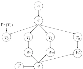
α ? θ ) @ @ @ R XX XX XX XX XXXz Pr (Y0) ? β - φ @ @ @ I : T0 T1 T2 Tn W1 W2 Wn ? ? ?

Figure 2.1: Latent Dirichlet Allocation Topic Model

Gibbs sampling is a class of MCMC algorithms which consists of repeatedly sampling each variable in our model from the conditional distribution given all the other variables. For example, if θ is a vector of parameters θ = θ1, θ2, ..., θk and e is the observation,

the Gibbs sampling algorithm samplesθ1 from Pr(θ1|θ2:k, e) followed by samplingθ2 from

Pr(θ2|θ1, θ3:k, e) all the way to θk, after which we start again from sampling θ1. It can be

shown that the resulting Markov chain has stationary distributionP(θ1, ..., θk|e).

Gibbs Sampling is very popular owing to its simplicity. However, one of the major obstacles with Gibbs Sampling is to decide on a stopping criterion.

2.4

Latent Dirichlet Allocation

Latent Dirichlet Allocation is a generative Bayesian model that describes a joint distribu-tion over the topics and words in a document corpus. It was introduced by Blei et. al. in [15]. Each word in each document is associated with a hidden topic. Let the total number of topics beT, the total number of documents be Dand the total words in the vocabulary be W. The number of words in documentd is Nd. We denote the hidden topic of the nth

word bytn. Then the model is is parametrized by the following distributions

• Word-Topic DistributionEach document dis represented by a multinomial topic distribution θd={θd,1, . . . , θd,T} where θd,t is the probability of topic t in document

(32)

• Document-Topic Distribution The distribution over words given a particular topic t is called the Topic-Word distribution and is denoted byφt ={φt,1, . . . , φt,W},

where W is the total number of words in the dictionary.

Each θd is usually modeled as a multinomial distribution and is sampled from a prior

f(θd;α). For LDA the prior is a Dirichlet distribution of the form

Dir(θd, αd) = Γ(PT i=1αd,i) QT i=1Γ(αd,i) n Y i=1 θαd,i−1 d,i 0≤θd,i ≤1 X i θd,i = 1 (2.13)

For a corpus, each φt is sampled from another priorg(φt;β) which is a dirichlet

parmater-ized by β. The nth _{word in document} _d _{can be generated by first sampling a topic} _t _from

θdand then sampling a word wn fromφt. We will use the following terminology frequently

for notational convenience Θ ={θ1, . . . , θD}

Φ ={φ1, . . . , φT}.

wa:b =wa, wa+1. . . wb a sequence of words from time a to b

ta:b =ta, ta+1. . . tb a sequence of hidden states from timea to b

Pn(Θ,Φ) = Pr (Θ,Φ|w1:n)

kn= Pr (wn|w1:n−1)

cn = Pr (w1:t)

2.4.1

Learning and Inference

In LDA, given a corpus, we are interested in identifying the mixture of topics pertaining to a particular document and estimating Θ and Φ. We can use Bayes rule to estimate Θ and Φ for a corpus by computing the posterior Pn(Θ,Φ) = Pr(Θ,Φ|w1:n) using Bayesian

(33)

Learning. If the nth _word_w

n lies in document d, the posterior can be calculated by

Let the prior P0(Θ,Φ) = f(Θ,Φ|α, β) be a distribution in θs and φs where α and β are

sets of parameters of the distributionf. Then according to Eq.2.14 the number of terms in the posterior grows by a factor ofT after each word due to the summation overt. After

n words, the posterior will consist of a mixture ofTn terms, which is intractable.

2.5

Dynamic Bayesian Networks

Dynamic Bayesian Networks are generative Bayesian models that describes a joint distri-bution over sequential data. Evidence is acquired at every time step and based on this evidence the values of the hidden variables are updated.

2.5.1

Hidden Markov Models

A Hidden Markov Model (HMM) is a DBN in which each observationet is associated with

a hidden stateyt that depicts some quantity of interest that is not observable directly. An

HMM is shown in Figure 2.2. In HMMs, the Markov assumption states that the current state is only dependent on the state at the previous time step. The Stationary process assumption states that the model parameters do not change over time. This setting is use-ful in many domains, including activity recognition, speech recognition, natural language processing. In activity recognition, activities are the hidden states and sensor measure-ments are the observations. The user performs a sequence of activities that are not directly observable but can be measured through sensors. Since the activities are not scripted nor

(34)

be desirable to learn the model parameters as the activities are performed, meaning that learning should be done in an online fashion. We denote the number of states by N and the number of observations by M. There are two distributions that represent this model

• Transition Model: The transition distribution models the change in the value of the hidden state over time. The distribution over the current state Yt given that the

previous state is y is denoted by θy = Pr (Yt|Yt−1 =y) where θy = {θy,1, . . . , θy,N}

and θy,i= Pr (Yt=i|Yt−1 =y) is the probability that the current state isigiven that

the previous state was y.

• Observation Model: The observation function models the effect of the hidden state on the observation at any given time t. The distribution over observations given a particular state is denoted by φy = Pr (Et|Yt=y) where φy = {φy,1, . . . , φy,M} and

φy,e = Pr (Et=e|Yt =y) is the probability that observation e is seen if the current

state is y.

To generate the observation sequence, for each y ∈ {1, . . . , N} we first sample θy from

a prior f(θy;αy) and φy from another prior f(φy;βy). Then we generate each observation

by first sampling the current statey0 from θy wherey is the state sampled at the previous

time step and then sample an observatione from φy0.

We will use the following terminology frequently for notational convenience Θ ={θ1, . . . , θN}

Φ ={φ1, . . . , φN}.

α set of hyperparameters for the transition distribution

β set of hyperparameters for the observation distribution

ea:b =ea, ea+1. . . eb a sequence of evidence from time a tob

ya:b =ya, ya+1. . . yb a sequence of hidden states from timea to b

(35)

α ? θ ) @ @ @ R XX XX XX XX XXXz Pr (Y0) ? β - φ @ @ @ I : Y0 Y1 Y2 Yn E1 E2 En - - - -? ? ?

Figure 2.2: A Bayesian Hidden Markov Model

2.5.2

Inference

There are 3 inference tasks that are typically performed with an HMM:

• Filtering : This is the task of computing the posterior over the hidden variables given all previous evidence by integrating out the parameters Θ and Φ. P r(Yt=y|e1:t,Θ,Φ)

can be computed using

• Smoothing: This is the task of computing the posterior distribution over a past state 0< k < t given all evidence up to time t: Pr (Yk =y|e1:t)

Pr (Yk=y|e1:t,Θ,Φ) =

1 Pr (e1:t|Θ,Φ)

Pr (Yk =y|e1:k,Θ,Φ) Pr (ek+1:t|Yk =y,Θ,Φ)

(2.17) This is also called the Baum Welch algorithm. It is important to note this posterior can not be computed online as it requires future observations. Pr (ek+1:t|Yk) can be

(36)

recursively calculated using Pr (ek+1:t|Yk =y,Θ,Φ) = N X Yk+1=1 Pr (ek+1|yk+1,Φ) Pr (ek+2:t|yk+1,Θ,Φ) (2.18) Pr (yk+1|Yk=y,Θ)

• Most likely explanation: This is the task of computing the most likely sequence of states that generated a particular sequence of observations argmaxy1:tPr (y1:t|e1:t).

This is also called the ”Viterbi Algorithm”. It can be calculated using the following recursive equation, max y1:t (Pr (y1:t, Yt+1 =y|e1:t+1,Θ,Φ)) (2.19) ∝Pr (et+1|Yt+1 =y,Φ) max yt Pr (Yt+1 =y|yt,Θ) max y1:t−1 (Pr (y1:t−1, yt|e1:t,Θ,Φ))

2.5.3

Bayesian Filtering

Filtering : In Bayesian Filtering, we compute the posterior over the hidden variables given all previous evidence P r(Yt = y|e1:t) by integrating Θ and Φ. We use the symbol cyt to

denote this posterior as defined in section2.5.1. We will see later that in Bayesian Learning for HMMs, this posterior will be used as a normalization constant.

2.5.4

Parameter Learning

(37)

• Supervised Maximum Likelihood Parameter Learning : If the values of both the hid-den variablesy1:T and the evidencee1:tare known, then learning from both sequences

is called ”supervised learning”. The optimal parameters Θ∗ and Φ∗ can be learned from data by maximizing the log likelihood of the data.

Θ∗,Φ∗ =argmaxΘ,Φlog (Pr (y1:T, e1:T|π, θ, ψ)) (2.21) subject to N X y0₌₁ θy0_,y = 1∀y ∈ {1, . . . , N} M X e=1 φy,e = 1∀y∈ {1, . . . , N}

This optimization problem has an analytical solution which we will discuss in subse-quent chapters.

• Unsupervised Maximum Likelihood Parameter Learning : If the values of the hidden variables are not available, then this is called unsupervised learning. Ideally we should

maximizeP

y1:tPr (y1:T, e1:T|Θ,Φ) over Θ and Φ. However this results in a non convex

optimization problem. Instead, we use the ”Expectation Maximization Algorithm” [13] which optimizes a convex approximation of this function by maximizing the expected value of the log likelihood

Θi+1,Φi+1 =argmaxΘ,Φ X y1:t Pr y1:T, e1:T|Θi,Φi log (Pr (y1:T, e1:T|Θ,Φ)) (2.22) subject to N X y0₌₁ θy0_,y = 1∀y ∈ {1, . . . , N} M X e=1 φy,e = 1∀y∈ {1, . . . , N}

Here we sum over all possible sequences y1:T where each yi = 1, . . . , N.

• Bayesian Learning in an HMM : In Bayesian Learning we calculate a posterior dis-tribution over the parameters given a prior disdis-tribution and the data using

Pr (Θ,Φ|e1:t) = X y Pr (Θ,Φ|Yt=y, e1:t) Pr (Yt=y|e1:t) = X y P_ty(Θ,Φ)cy_t (2.23)

(38)

Using Bayes Rule, P_ty(Θ,Φ) (2.24) = Pr (Θ,Φ|Yt=y, e1:t) = Pr (Θ,Φ, Yt=y, e1:t) Pr (Yt=y, e1:t) = Pr (et|Yt=y,Φ) Pr (Yt =y, et|e1:t−1) N X i=1 Pr (Yt=y|Yt−1 =i,Θ) Pr (Θ,Φ, Yt−1 =i|e1:t−1) Pr (Yt−1 =i|e1:t−1) = (1/k_ty)φy,et N X i=1 θi,ycit−1P i t−1(Θ,Φ) where k_ty = Z Φ,Θ φy,et X i θi,ycit−1P i t−1(Θ,Φ)dΦdΘ (2.25)

We can also calculate the posterior Pr (Yt=y|e1:t) = cyt =k y t/ P ik i t.

Let the priorP0(Θ,Φ) = f(Θ,Φ|α, β) be some distribution inθs andφs whereαand

β are the parameters of the distribution f. Then according to Eq. 2.24 the number of terms in the posterior grows by a factor of N after each observation due to the summation over i. After t observations, the posterior will consist of a mixture of Nt

terms, which is intractable. In the next Chapters we will discuss how to approximate this posterior in an online fashion.

2.6

Conditional Random Fields

Conditional Random Fields (CRFs) are an alternative to HMMs [46]. Unlike HMMs, CRFs are discriminative, i.e., they model only the conditional distribution of the hidden variables given the evidence. An important advantage of this approach is that there are no assumptions on the distribution of the evidence.

Definition 2.6.1. A clique in an undirected graph is a subset of its vertices such that every two vertices in the subset are connected by an edge.

(39)

Given a set of observable random variables E1:t and hidden variables Y1:t, a CRF can

be defined by a tuple (E, Y,G,F, λ). Here G is an undirected graph with vertices V

corresponding to the random variables and a set of cliques C that model the interactions between them. F = (fC)C∈C is a family of real valued functions. For every clique C ∈ C

that has vertices EC and YC,

fC :EC×YC→R

n(C) _(2.26)

wheren(C)∈ {1,2, . . .} is the dimension of the feature vector,_E_C is the set of all possible assignments to nodes in EC and YC is the set of all possible assignments to nodes in YC. For allC ∈ C,λC ∈Rn(C)is a family of weights. Usually the feature functions of a CRF are

fixed while the weights are learned from data. The probability of Y1:T = y1:T conditioned

one1:T is given by Pr λ(y1:t|e1:t) = 1 Zλ(e1:t) exp ( X C∈C λCfC(eC, yC) ) (2.27)

The normalization constant can be evaluated as

Zλ(e1:t) = X y1:t∈Y1:t exp ( X C∈C λCfC(eC, yC) ) (2.28)

2.6.1

Linear Chain CRF

In a linear chain CRF with observations e1:T and labels y1:T, the set of cliques C is given

by C = {{et, yt}∀t ∈ {1, . . . , T}} ∪ {{yt, yt−1},∀t ∈ {2, . . . , T}}. The CRF includes two

kinds of feature functionsft(et, yt) = f(et, yt) with weightλt=µandft−1,t(e1:t, yt−1, yt) =

g(yt−1, yt) with weight λt−1,t=ν. Pr (y1:t|e1:t) = 1 Zλ(e1:t) exp ( X C∈C λCfC(eC, yC) ) (2.29) = 1 Zλ(e1:t) exp ( _T X t=1 µf(et, yt) + T X t=2 νg(yt−1, yt) )

(40)

Inference

For inference in a CRF, letM be a|_Y| × |_Y| matrix, such that

Mt(i, j) = exp{µ f(et, j) +ν g(i, j)} (2.30)

We can use a Baum-Welch type procedure similar to the HMM and use the following recursions to generate the forward and backward messages

αy(1) =µ f (e1, y) αy(t) =αt−1Mt t= 2, . . . , T (2.31)

βy(N) =1 βy(t) =αt−1Mt+1βtT+1 t =T −1, . . . ,1 (2.32)

It can be shown thatZλ =P_y∈Yαy(T).

Parameter Learning

Learning the parameters of the CRF corresponds to learning the weightsµ and ν of each feature function. We setup the following optimization problem to maximize the conditional log likelihood of the data

arg max_µ,ν −log (Zλ(e1:T)) + T X t=1 µ f(et, yt) + T X t=2 ν g(yt−1, yt)− λTλ 2σ2 ! (2.33)

The last term on the right hand side is a regularizer which penalizes large weights. In a Bayesian framework, it can be regarded as a Gaussian prior with mean 0, varianceσ2 _and

all weights are uncorrelated. This is a convex optimization problem and can be solved using gradient based search.

(41)

Chapter 3

Related Work

In this chapter, we review some of the techniques that have been previously used for Bayesian learning. We also review the literature in the context of Latent Dirichlet Alloca-tion Models as well as models for activity recogniAlloca-tion with instrumented devices.

3.1

Parameter Learning for Latent Dirichlet

Alloca-tion

One of the main challenges in Bayesian learning is that the posterior distribution can become very complex as new information becomes available. In some cases, the posterior can be an exponentially large mixture of distributions. Hence representing the posterior and calculating its statistics can be computationally expensive. Typically algorithms aim to construct an approximate posterior.

We have described Gibbs Sampling [52] briefly in the previous section. Griffiths et. al. [34] use Gibbs Sampling to estimate the parameters of the LDA model. Gibbs Sampling is popular for its simplicity and its ability to produce good estimates. The algorithms passes over the data multiple times, however to process each observation, it only requires

O(n) time where n is the number of hidden states. One of the major weaknesses of Gibbs Sampling is that convergence of the Markov chain is difficult to detect reliably. In addition to that, the stochastic nature of the algorithm leads to estimates that vary with each run. Another popular class of techniques called Variational Bayesian techniques construct

(42)

posterior and a simpler distribution. The latent nature of the hidden variables leads to a non-convex optimization problem, therefore, instead of minimizing the KL divergence, an upper bound of the KL divergence is optimized. For LDA Variational Bayes exploits the exchangeability assumption and is able to process multiple occurrences of the same word in a document at the same time. Variational Bayes methods can be much faster than sampling based approaches but tend to underestimate the posterior variance[14]. Blei et. al. [15] have utilized Variational Bayesian techniques to learn the parameters of the LDA Model.

Spectral learning algorithms([8],[7],[16],[42]) are based on spectral decomposition of mo-ment matrices or other algebraic structures of the model. In Excess Correlation Analysis [7] the parameters are estimated by matching the moments of the model with the empirical moments. The technique is computationally simple (e.g., matrix operations and singular value decomposition) and it ensures consistency. Despite its theoretical guarantees, ECA often generates negative probabilities. This arises from the fact that ECA does not en-force non-negative solutions (which would be NP-hard) and the empirical moments are necessarily approximations of the true underlying moments.

Most of the above mentioned algorithms require the complete data to be present in the memory at the time of learning and usually require the model to be retrained if new data arrives. This can be problematic for large data sets and applications where new data becomes available frequently. The Moment Matching algorithm that is proposed in this thesis is an online technique which means that updating the model parameters after receiving each new observation requires a constant amount of time.

3.1.1

Online Parameter Learning for LDA

More recently, online versions of some of the algorithms mentioned above have been devel-oped that are able to incorporate new information without retraining the complete model. The Online Variational Bayes algorithm [40] and the sparse stochastic online inference algo-rithm [54], both utilize online stochastic optimization to compute an approximate posterior distribution for LDA. At each iteration, these methods sample some documents from the corpus and then update the parameters by taking a step in the direction of the gradient that minimizes KL divergence between the approximate posterior and the exact poste-rior. The authors show that the algorithm converges to a local optimum of the variational bound. However, these algorithms suffer from the same limitation as offline Variational Bayes. In addition to that, the approximation produced by these algorithms is only as good as a single pass of the Variational Bayes algorithm and therefore they require a lot of data to produce reasonable estimates.

(43)

3.2

Activity Recognition for Instrumented Walker

There has been some previous work for activity recognition with instrumented walkers. In [6] the authors describe a method that assesses basic walker assisted gait characteristics. Their model is based on the measurement of weight transfer between the user and the walker by two load cells in the handles of the walker. They use a total of 8 participants for their experiments with each users performing a total of 50 experiments emulating 16 navigational scenarios including walking, turns and docking to a chair. A simple thresh-olding approach is used to detect peaks and valleys in the load measurements, which are assumed to be indicative of certain events in the gait cycle. This work focuses on low level gait statistics where as we are interested to recognize complex high level activities. Hirata et. al. [39] instrumented a walker with sensors and actuators. They recognize three user states: walking, stopped and emergency (including falling). These states are inferred based on the distance between the user and the walker (measured by a laser range finder) and the velocity of the walker. This work is limited to the three states mentioned above and would not be able to differentiate between activities that exhibit roughly the same velocity and distance measurements (e.g., walking, turning, going up a ramp).

A significant amount of work has been done on activity recognition in other contexts. In particular, Liao et. al. [49] use a Hierarchical Markov Model to learn and infer a user’s daily movements through an urban community. The model uses multiple levels of abstraction in order to bridge the gap between raw GPS sensor measurements and high level information such as a user’s destination and mode of transportation. They use Rao-Blackwellized particle filters for state estimation.

Patel et. al. [62] have designed a walker equipped with the following sensors namely, IRt (Infra-red Torso), IRw (Infra-red Waist), LSG (Left Strain Gauge), RSG (Right Strain Gauge), RF (wireless Radio Frequency switch), LOC (Localisation) and TOD (Time-of-Day). They generate artificial data for a users navigating through a home. They use a Dynamic Bayesian Network and an SVM to do activity recognition. Their work is inspired by the work presented in Chapter 6 and in [61].

3.2.1

Parameter Learning in HMM

Parameter Learning in time series data is a challenging problem. Many of the methods described in the previous section have also been used for parameter learning in HMMs. Beal [11] has used Variational Bayes to learn the parameters of an HMM with discrete

(44)

A popular class of methods for learning the parameters of an HMM is a technique called Expectation Maximization which finds point estimates of the parameter values such that the expected likelihood of the observed data is maximized [13]. We have introduced this algorithm in the previous section. In expectation maximization, a concave under-estimator of the log likelihood is maximized. Expectation Maximization is also an offline technique which means that the full data is required to be in the memory for learning and multiple passes are required for the algorithm to converge. EM is useful for several reasons: conceptual simplicity, ease of implementation, and the fact that each iteration improves the value of the parameters. The rate of convergence on the first few steps is typically quite good, but can become slow as you approach a local optimum. Generally, EM works best when the fraction of missing information is small and the dimensionality of the data is not too large. EM can require many iterations, and higher dimensionality can dramatically slow down the E-step [69].

An online version of the Expectation Maximization algorithm for discrete Hidden Markov Models has been developed by Mongillo et. al. [57]. Cappe et. al. have also derived an online EM algorithm for HMMs with Gaussian observation distribution. Both of these require O(n4 +n3×m) operations at every time step where n is the number of hidden states and m is the number of observations. In comparison to this, I have pro-posed a version of the Moment Matching algorithm that only requires O(n) operations at every time step. Both Mongillo and Cappe provide a limited analysis of their work using synthetic data with n= 2.

Foti et. al [28] have also derived an Online Variational Bayes algorithm for learning the parameters of an HMM with discrete states and Gaussian observation distribution. In order to break the dependencies in the chain, they consider mini-batches of observations which seems natural in Bayes nets where the exchangeability assumption holds, however for HMMs it creates edge cases and breaks dependencies between consecutive hidden states at the start and end of a mini-batch. In order to tackle this, Foti, et. al. buffer some observations before and after the mini-batch and make the assumption that the sub-chain is representative of the full time series chain. Their algorithm harnesses the memory decay of the chain to adaptively bound errors arising from edge effects. They have demonstrate the effectiveness of their algorithm on synthetic experiments and a large genomics dataset. In their implementation, they assume a Gaussian observation distribution which allows them to make efficient updates at every time step.

(45)

3.3

Assumed Density Filtering

The moment matching algorithm described in this thesis is very close to Assumed Density Filtering. In Assumed Density Filtering, KL divergence between an approximate posterior and the exact one is minimized [55]. This leads to matching the natural moments of the distribution. Alamino et. al [5] have explored this approach to learn the parameters of a discrete HMM with Dirichlet priors. For Dirichlet priors, matching the natural moments involves solving multiple systems of non linear equations which is a computationally in-tensive process. The authors have suggested matching the first and second order moments which can be done by solving a linear system of equations that have an analytical solution. However, they do not provide any explanation for why this is a good idea and how this will affect the convergence properties of the algorithm. In addition to that, they do not handle the state switching problem that we have described previously. In this thesis, I provide an alternative argument for matching the first and second order moments. Matching the first and second order moments allows us to define higher order moments in terms of an implicit prior such that if we did exact inference with respect to the implicit prior, then the value first order moment of the posterior will be the same as the one acquired by starting with a different prior and doing moment matching to compute the posterior. In addition to that, each new observation can be incorporated in time linear in the number of hidden states which has not been discussed before in terms of ADF. I also provide an explicit treatment for state switching that is ignored in ADF.

Minka et. al.[55],[56] have proposed an algorithm called Expectation Propagation where they use an iterative technique that repeatedly approximates the posterior over all hidden variables with a simple distribution by matching a few moments of the posterior for in-ference. This step is then embedded in an EM algorithm for learning. The convergence properties of this approach are not well understood and when convergence arises it is very slow. In practice the algorithm is very slow and does not scale well to large data sets for the case of LDA.

All of the above techniques have been used with success in practice, however they are each approximate and further approximations must be done to obtain online algorithms that perform a single scan of the data. In this thesis, I present an online Bayesian moment matching (BMM) technique which is simple to implement and it outperforms existing techniques both in terms of accuracy and time and is exact with respect to an implicit prior. In the next chapter I will describe the motivation and framework for Bayesian Moment Matching.

(46)

Chapter 4

Online Bayesian Learning Using

Moment Matching

In this chapter I describe a technique for Bayesian learning called Bayesian Moment Match-ing (BMM) which is based on Assumed Density FilterMatch-ing (ADF). The main idea is to update the poster